INTRODUCTION
The East Asian monsoon (EAM), comprising the East Asian summer monsoon (EASM) and East Asian winter monsoon (EAWM), is an important component of the Earth's climate system and has a significant influence on the socioeconomic and cultural development of East Asia. Its evolution has been widely studied via the analysis of the response of cave stalagmites (Wang et al., Reference Wang, Cheng, Edwards, He, Kong, An, Wu, Kelly, Dykoski and Li2005, Reference Wang, Cheng, Edwards, Kong, Shao, Chen, Wu, Jiang, Wang and An2008; Hu et al., Reference Hu, Henderson, Huang, Xie, Sun and Johnson2008; Cai et al., Reference Cai, Tan, Cheng, An, Edwards, Kelly, Kong and Wang2010), loess–paleosol profiles (Sun et al., Reference Sun, An, Su, Lu and Sun2003, Reference Sun, An, Clemens, Bloemendal and Vandenberghe2010; Kang et al., Reference Kang, Wang, Roberts, Duller, Cheng, Lu and An2018), lacustrine sediments (Yancheva et al., Reference Yancheva, Nowaczyk, Mingram, Dulski, Schettler, Negendank, Liu, Sigman, Peterson and Haug2007; An et al., Reference An, Colman, Zhou, Li, Brown, Timothy Jull and Cai2012; Chen et al., Reference Chen, Xu, Chen, Birks, Liu, Zhang and Jin2015), and marine sediments (Xiao et al., Reference Xiao, Li, Liu, Chen, Xie, Jiang, Li, Xiang and Chen2006; Liu et al., Reference Liu, Dong, Yang, Herzschuh, Zhang, Stuut and Wang2009; Huang et al., Reference Huang, Tian and Steinke2011; Sagawa et al., Reference Sagawa, Kuwae, Tsuruoka, Nakamura, Ikehara and Murayama2014; Hao et al., Reference Hao, Liu, Ogg, Liang, Xiang, Zhang, Zhang, Zhang, Liu and Li2017) to global climate changes. The study of the evolution of the EAM during the Holocene has been improved with the acquisition of high-resolution sedimentary records in recent years. However, previous studies have found that the evolution of the EAM has significant regional response characteristics.
A pollen record in Gonghai Lake revealed that the EASM gradually strengthened during the early-middle Holocene and weakened during the late Holocene (Chen et al., Reference Chen, Xu, Chen, Birks, Liu, Zhang and Jin2015). Records from lake deposits in Qinghai Lake and stalagmites in Dongge Cave manifest a weakening of the EASM during the Holocene (Wang et al., Reference Wang, Cheng, Edwards, He, Kong, An, Wu, Kelly, Dykoski and Li2005; An et al., Reference An, Colman, Zhou, Li, Brown, Timothy Jull and Cai2012). Similarly, the EAWM also shows an asynchronous evolutionary trend. A weakening trend of the EAWM during the Holocene is recorded in the South China Sea (Hu et al., Reference Hu, Yang, Zhao, Yoshiki, Fan and Wang2012; Huang et al., Reference Huang, Tian and Steinke2011; Steinke et al., Reference Steinke, Glatz, Mohtadi, Groeneveld, Li and Jian2011), while an enhanced trend is recorded in the East Asian marginal sea (Zheng et al., Reference Zheng, Li, Wan, Jiang, Kao and Cody2014; Hao et al., Reference Hao, Liu, Ogg, Liang, Xiang, Zhang, Zhang, Zhang, Liu and Li2017). The nonuniformity of the monsoon variation may be attributed to the different responses of sedimentary environments to monsoonal change and/or the sensitivity of various monsoon proxies. Therefore, more evidence is needed for the study of the EAM's evolution during the Holocene. It is generally considered that the development of the EAM is caused by the temperature gradient between the Eurasian continent and the Indo-Pacific Ocean (Wang et al., Reference Wang, Cheng, Edwards, He, Kong, An, Wu, Kelly, Dykoski and Li2005, Reference Wang, Li, Lu, Gu, Rioual, Hao and Mackay2012; Hu et al., Reference Hu, Yang, Zhao, Yoshiki, Fan and Wang2012; Sagawa et al., Reference Sagawa, Kuwae, Tsuruoka, Nakamura, Ikehara and Murayama2014; Wen et al., Reference Wen, Liu, Wang, Cheng and Zhu2016; Huang et al., Reference Huang, Zeng, Ye and Wei2019). In recent decades, other forcing factors, such as the El Nino–Southern Oscillation (ENSO), the Intertropical Convergence Zone (ITCZ), and North Atlantic forcing related to the Atlantic Meridional Overturning Circulation (AMOC), have been proposed to drive the EAM's evolution (Bond et al., Reference Bond, Kromer, Beer, Muscheler, Evans, Showers, Hoffmann, Lotti-Bond, Hajdas and Bonani2001; Yancheva et al., Reference Yancheva, Nowaczyk, Mingram, Dulski, Schettler, Negendank, Liu, Sigman, Peterson and Haug2007; Hoffman and Jeremy, Reference Hoffman, Carlson, Winsor, Klinkhammer, LeGrande, Andrews and Strasser2012; Shi et al., Reference Shi, Liu and Cheng2012; Zheng et al., Reference Zheng, Li, Wan, Jiang, Kao and Cody2014; Böhm et al., Reference Böhm, Lippold, Gutjahr, Frank, Blaser, Antz, Fohlmeister, Frank, Andersen and Deininger2015; Zhao et al., Reference Zhao, Wan, Song, Gong, Zhai, Shi and Li2019). The study of high-resolution regional climate evolution provides evidence for understanding global climate change during the Holocene.
The South Yellow Sea (SYS) is a semiclosed epicontinental sea located north of the East China Sea, with an average water depth of ~44 m at present. Its sedimentary environment is strongly influenced by the EAM system. The central muddy area is the main sediment “sink” and has a weak hydrodynamic environment (Liu et al., Reference Liu, Millimam, Gao and Cheng2004; Li et al., Reference Li, Li, Liu, Qiao, Ma, Xu and Yang2014a; Zhou et al., Reference Zhou, Dong and Li2015). Relatively minor changes in climate are likely to be archived in the sedimentary record in this sensitive region. Therefore, the SYS has been regarded as an ideal location for studying the evolution of the EAM, and several studies have targeted the reconstruction of the EAWM (Hu et al., Reference Hu, Yang, Zhao, Yoshiki, Fan and Wang2012; Hao et al., Reference Hao, Liu, Ogg, Liang, Xiang, Zhang, Zhang, Zhang, Liu and Li2017). Coarse sensitive fractions of muddy sediments recorded that the EAWM experienced strong (7.2–4.2 ka), moderate (4.2–1.8 ka), and weakened (1.8–0 ka) periods during the Holocene, and the intensified events correlate well with the North Atlantic ice-rafted debris (IRD) events (Hu et al., Reference Hu, Yang, Zhao, Yoshiki, Fan and Wang2012). Hao et al. (Reference Hao, Liu, Ogg, Liang, Xiang, Zhang, Zhang, Zhang, Liu and Li2017) constructed century-scale variation in the EAWM for the past 6.3 ka using the high-frequency variability in lignin records and proposed that North Atlantic climate forcing has a significant effect on EAWM variability at centennial time scales. In contrast, the delivery of lignin in the SYS is mainly influenced by the Yellow Sea Warm Current (YSWC), which is not only driven by the EAWM winds but also greatly affected by the Kuroshio Current (Hao et al., Reference Hao, Liu, Ogg, Liang, Xiang, Zhang, Zhang, Zhang, Liu and Li2017). Moreover, grain-size characteristics in sediments from some muddy areas can be influenced by riverine runoff and storms as well as coastal currents (Tu et al., Reference Tu, Zhou, Cheng, Liu, Yang and Wang2017; Tian et al., Reference Tian, Fan, Zhang, Chen, Wang, Liu and Yang2019). Thus, how the SYS responds to the EAWM variations and whether the sedimentary strata in the SYS record the changes in the EASM requires further study using high-resolution continuous sedimentary records.
In our study, we focused on high-resolution (~10 yr spacing on average) sediment records from the western central muddy area of the SYS to elucidate the evolution of the EAM during the Holocene. Clay mineral assemblages were used to determine the sediment provenance in the western SYS. The C37 long-chain alkenone thermometer (${\rm U}{{K^{\prime}} \over {37}}$ ) and grain sizes, which have been widely used in marine sediment research (Xiao et al., Reference Xiao, Li, Liu, Chen, Xie, Jiang, Li, Xiang and Chen2006; Li et al., Reference Li, Nan, Jiang, Sun, Zhang and Li2009; Hu et al., Reference Hu, Yang, Zhao, Yoshiki, Fan and Wang2012; Tao et al., Reference Tao, Xing, Luo, Wei, Liu and Zhao2012; Yi et al., Reference Yi, Yu, Ortiz, Xu, Chen, Ge, Hao, Yao, Shi and Peng2012; Zhou et al., Reference Zhou, Sun, Huang, Cheng and Jia2012; Sagawa et al., Reference Sagawa, Kuwae, Tsuruoka, Nakamura, Ikehara and Murayama2014; Ruan et al., Reference Ruan, Xu, Ding, Wang and Zhang2015; Nan et al., Reference Nan, Li, Chen, Chang, Yu, Xu and Pi2017), were used to construct the processes of environmental evolution in the SYS. The evolution of the EAM during the Holocene was reconstructed in this study, and the phase relationship and dynamic mechanism of the EAWM and EASM at different time scales are discussed via comparison with different regional climate records.
REGIONAL SETTINGS
The Yellow Sea, located between mainland China and the Korean Peninsula, covers an area of ~38 × 104 km2 (He, Reference He2006). Its hydrology manifests in clear seasonal variations, with the appearance of warm and saline tongue structures in winter and a cold-water mass that occupies the central Yellow Sea below the thermocline in summer (Lee et al., Reference Lee, Pang and Moon2016; Tak et al., Reference Tak, Cho, Seo and Choi2016). The Yellow Sea is divided into two parts: the North Yellow Sea (NYS) and the SYS, with the Shandong Peninsula separating the two. Two general circulation patterns in the SYS are reported: a counterclockwise gyre in the western part and a clockwise gyre in the eastern part (Tak et al., Reference Tak, Cho, Seo and Choi2016). The former consists of a northward inflow of the YSWC and a southward inflow of the Yellow Sea Coastal Current (YSCC), and the latter consists of the YSWC and a southward inflow of the Korea Coastal Current (KCC; Fig. 1). The YSCC and KCC are typical wind-induced currents that flow southward throughout the year. The intensity of the YSWC gradually weakens from the seafloor to the sea surface (Tak et al., Reference Tak, Cho, Seo and Choi2016). Two warm current branches were found in the north and northwest based on the statistical results of sea-surface temperature (SST) in the Yellow Sea (Zhao et al., Reference Zhao, Yu, Diao and Si2011). Moreover, the YSWC originates from a tongue-shaped, high-salinity body of warm water that extends from the southwestern Cheju Island to the Yellow Sea (Fig. 1), and its formation depends on the Kuroshio Current and monsoon, with contributions of two-thirds and one-third, respectively (Song, et al., Reference Song, Bao, Wang, Xu, Lin and Wu2009; Xu et al., Reference Xu, Wu, Lin and Ma2009a).

Figure 1. Maps of the study area in the western North Pacific and regional surface current system. (a) The locations of the Yellow Sea, East China Sea, and South China Sea; the sphere of influence of the Asian monsoon; and the mean location of the westerly jet stream. The red box represents the area shown in b. (b) The ocean circulation of the region (modified from Nan et al., Reference Nan, Li, Chen, Chang, Yu, Xu and Pi2017). The red lines indicate the warm current systems and the blue lines indicate the cold coastal currents. Shaded areas represent the muddy areas, namely: 1, the Shandong mud wedge; 2, the central muddy deposit of the SYS; and 3, the southwest muddy deposit of Jeju Island. BS, Bohai Sea; NYS, North Yellow Sea; SYS, South Yellow Sea; ECS, East China Sea; SCS, South China Sea; KCC, Korean Coastal Current; YSCC, Yellow Sea Costal Current; YSWC, Yellow Sea Warm Current; TC, Tsushima Current; SPCC, Shandong Peninsula Coastal Current; CDW, Changjiang Diluted Water; KC, Kuroshio Current; TWC, Taiwan Warm Current; SEC, Shelf Edge Current. Orange crosses show the locations of the climate proxy records in the monsoon region. (For interpretation of the references to color in this figure legend, the reader is referred to the web version of this article.)
The leading factor controlling sediment resuspension, transport, and deposition by the tidal current in the Yellow Sea was previously determined using a model combined with in situ observations (Dong et al., Reference Dong, Su and Wang1989; Lee and Chu, Reference Lee and Chu2001). A weak tidal current in the central SYS corresponds to a muddy deposition, while a strong tidal current is responsible for sand deposition (Yang et al., Reference Yang, Jung, Lim and Li2003; Li et al., Reference Li, Li, Liu, Qiao, Ma, Xu and Yang2014a; Zhou et al., Reference Zhou, Dong and Li2015). The Huanghe and Yangtze River are considered the two major sediment sources for the Yellow Sea due to their high suspended sediment loads, which are ~9.8 × 10⁸ (Datong station; Ye, Reference Ye2019) and ~3.7 × 10⁸ tons (Tongguan station; Ye, Reference Ye2019), respectively. Simulation results revealed that most of the sediment in the muddy area of the central SYS originates from the Old Huanghe delta and the Yangtze River, while modern Huanghe sediment provides the smallest contribution (Bian et al., Reference Bian, Jiang and Greatbatch2013; Lu et al., Reference Lu, Li, Zhang and Huang2019). Although the sediment transport process on the continental shelf is characterized by a “store in summer, transport in winter” pattern (Qiao et al., Reference Qiao, Wang, Liu, Li, Liu, Huang, Xue and Zhong2017), some sedimentation based on events such as floods and typhoons also plays a pivotal role in muddy areas with low sedimentation rates (Tu et al., Reference Tu, Zhou, Cheng, Liu, Yang and Wang2017; Tian et al., Reference Tian, Fan, Zhang, Chen, Wang, Liu and Yang2019). Normally, the influence of the coastal current of the Yellow Sea transports the suspended sediments along the northern coast of Jiangsu Province to the southwest in winter, mixes them with Yangtze River sediments carried by diluted water, and then brings them into the central SYS, blocked by the YSWC in the southern SYS (Bian et al., Reference Bian, Jiang and Greatbatch2013; Gao et al., Reference Gao, Qiao and Li2016).
MATERIALS AND METHODS
Core YS01 (35°30′N, 122°30′E, 30.09 m in length, 58.5 m water depth), with an average sedimentation rate of ~0.113 cm/yr, was retrieved from the western central muddy area of the SYS in 2006 by R/V K407. The recovery rate of the sediment was 95% on average. The core was split, photographed, described, and sampled in the laboratory to obtain its sedimentological parameters in order to characterize the sedimentary environment.
14C accelerator mass spectrometry dating for core YS01
Large foraminiferal shells were difficult to find in the sediment; most shells found were those from the larvae of benthic foraminifera. Fourteen sample ages were obtained via 14C accelerator mass spectrometry dating of the shells of mixed benthic foraminifera; the analyses were tested four times in the Woods Hole Oceanographic Institution, Woods Hole, MA, USA, and the Beta Analytic Company, Miami, FL, USA. All ages were recalibrated. The sediment near the bottom bed was disturbed during drilling, resulting in the loss of samples at the top of the borehole core. The depth–age model for the core was established based on corrected calendar years using Calib Rev v. 7.0.4 software, the marine calibration curve Marine13, and a reservoir correction of approximately −139 ± 59 yr for the SYS (Southon et al., Reference Southon, Kashgarian, Fontugne, Metivier and Yim2002; Fig. 2, Table 1). All ages in this paper are reported as calibrated calendar 14C ages before AD 1950.

Figure 2. Sedimentary characteristics of borehole core YS01. (a) Lithologic log for 0–11 m in depth. Ages were obtained by AMS 14C dating. SC, silty clay; CSi, clayey silt; S-Si-C, sand–silt–clay; S, sand. (b) Sedimentation rate (m/ka, blue line). (c) Age–depth model (red line). (d) Content of sand fractions (%). (e) Content of silt fractions (%). (f) Content of clay fractions (%). (g) Mean grain size (μm). h) Sorting. (i) Size–frequency plots and cumulative probability plots for sediments at 1.0 m, 3.0 m, 7.0 m, and 10.0 m. (For interpretation of the references to color in this figure legend, the reader is referred to the web version of this article.)
Table 1. AMS radiocarbon dating results.

a a1, a2: the first and second dating, Woods Hole Oceanographic Institution, Woods Hole, MA, USA; b1, b2: the third and fourth dating, Beta Analytic Radiocarbon Dating Laboratory, Miami, FL, USA.
Grain-size analysis
A total of 1081 grain-size samples were spaced at 1 cm, with a mean time resolution of ~9 yr. Particle-size analysis was conducted at the Lab of Qingdao Marine Geology Institute, China Geological Survey, Qingdao, China, using a Malvern Mastersizer 2000 laser particle-size analyzer. The detrital fraction of the sediment was isolated from the bulk sediment after removing the organic matter and carbonates using 5 ml of 30% hydrogen peroxide and 5 ml of 10% hydrochloric acid, respectively. All samples were then soaked with neutral distilled water and washed three times in a centrifuge. The treated samples were dispersed in an ultrasonicator for 50 s. A particle-size analyzer was used for grain-size analysis with a measurement range of 0.02–2000 μm, a size resolution of 0.01 Φ, and an error of less than 3%.
${\rm U}{{K^{\prime}} \over {37}}$ –based temperature

A total of 526 samples were extracted from 2-cm-thick slices taken from the core and measured at the Marine Organic Geochemistry Laboratory, Ocean University of China, Qingdao, China. The ${\rm U}{{K^{\prime}} \over {37}}$ index was converted given the relative abundance of the diunsaturated (C37:2), triunsaturated (C37:3), and tetraunsaturated (C37:4) methyl ketones of carbon 37 and calculated based on the equation ${\rm U}{{K^{\prime}} \over {37}}$
 = (C37:2 − C37:4)/(C37:2 + C37:3 + C37:4). The C37:4 alkenone is rarely detected in low- to midlatitude marine sediments and only becomes abundant when the temperature is very low (<4°C). The ${\rm U}{{K^{\prime}} \over {37}}$
 index can therefore usually be simplified to the following expression: ${\rm U}{{K^{\prime}} \over {37}}$
 = C37:2/(C37:2 + C37:3). The extracts were hydrolyzed in KOH-MeOH solution, and then separated with silica gel cartridges. After derivatization by nitrogen, the O-Bis(trimethylsilyl)trifluoroacetamide and alkenones within the alcohol subfraction were analyzed by gas chromatography. Biomarker identification and structure verification were performed using thermo gas chromatography/mass spectrometry. Quantification of the biomarkers was carried out on an Agilent 6890N gas chromatographer using an HP-1 column (50 m) and with H2 as the carrier gas at 1.2 ml/min. The formula SST = ${\rm U}{{K^{\prime}} \over {37}}$
 × 0.033 + 0.044 (Müller et al., Reference Müller, Kirst and Ruhland1998) was used to convert ${\rm U}{{K^{\prime}} \over {37}}$
 into SST at an analytical resolution of 0.3°C.
Clay mineral analyses
Samples used for clay mineral analyses were taken at ~6 cm intervals; 146 samples were obtained and analyzed in total. The <2 μm fractions of each sample were separated by the Stoke's settling velocity principle and concentrated by centrifuging after the carbonate and organic matter were removed using 30% H2O2 and 10% HCl, respectively. Clay minerals were measured with standard X-ray diffraction on a D8 ADVANCE diffractometer at Qingdao Institute of Bioenergy and Bioprocess Technology, Chinese Academy of Sciences, Qingdao, China. The semiquantitative estimation of clay mineral abundances was based on the weighted peak areas of smectite (17 Å), illite (10 Å), and kaolinite/chlorite (7 Å) of the glycolated curve (Esquevin, Reference Esquevin1969) using MDI Jade v. 6.5 software. Relative proportions of kaolinite and chlorite were determined based on the ratio from the 3.57/3.54 Å peak areas. The chemical index of illite was assessed by measuring the intensity ratio of the 5 Å and 10 Å illite peaks. An illite chemistry index below 0.5 represents Fe-Mg–rich illite characterized by physical erosion, whereas an index above 0.5 is found in Al-rich illite formed by strong hydrolysis (Esquevin, Reference Esquevin1969).
RESULTS
Core lithology and chronology of core YS01
Sedimentary succession can be divided into four depositional units based on the lithology and sedimentary structure of the core, including two shallow-marine facies and two continental facies (Wang et al., Reference Wang, Li, Xu, Liu, Qiao, Ding, Yang, Dada and Li2019). The analyses presented in this paper mainly focus on the 0–10.8 m interval in order to reveal the response of sedimentary records in the SYS to climate change during the Holocene (Fig. 2). Water content is relatively high in sediments and can reach up to 59.6%.
For convenience, we used the core to describe the context. This unit is characterized by gray or taupe clayey silt with horizontal bedding, and organic matter spots and shell fragments are scattered throughout. Thin shelly layers, organic matter strips, and silty clay layers are common. The chronostratigraphic framework of the core was reconstructed based on AMS 14C measurements (Jia et al., Reference Jia, Li, Yu, Zhao, Xiang, Li, Zhang and Zhao2019; Fig. 2c; Table 1). The dating points were conducted at 0.9 m intervals on average and yielded a basal age of ~9.5 ka. The average resolution of the record is about 10 yr owing to the 1 cm sampling intervals. The result of AMS 14C dating suggests that the strata did not reverse during this period, which further suggests a stable sedimentary environment in the study area. Based on the 14 measured 14C ages, sediment accumulation rates between the dated horizons range from 0.3 to 4.1 m/ka. The average sedimentation rate of the core is 1.13 m/ka. A high sedimentation rate was identified at 3.2–4.2 m and 6.9–7.8 m (Fig. 2b).
Grain size
The sediments have little grain-size variation in this unit, ranging from 3.7 to 7.6 μm (Wang et al., Reference Wang, Li, Xu, Liu, Qiao, Ding, Yang, Dada and Li2019; Fig. 2g). Clay and silt contents range from 29.1% to 50.3% and 49.7% to 69.5%, respectively. Anticorrelations exist between clay and silt, which have a mean content of 38.0% and 61.7%, respectively. The content of sand is low, with an average of 0.3%; only a few layers exceed 1%. The result for sediment grain-size parameters shows that sediment sorting is closely related to grain size and that good sorting corresponds to a fine grain size (Fig. 2g and h).
The division of the core into three stages is supported by vertical changes in grain size. Sediments were characterized by coarse grain size (average sand component: 0.6%) and high frequency variation at the 6.3–10.8 m interval, with an average mean grain size of 5.9 μm. Mean grain size began to decrease and sorting gradually became better in the following interval of 1.4–6.3 m. The average content of sand and silt decreased by 0.5% and 4.5%, respectively. The last interval (0–1.4 m) is characterized by a coarsening of sediment grain size and poor sorting, and the components near the median grain size account for a large proportion of the sediment (Fig. 2g and h). The grain-size distribution of the terrigenous fraction in the core exhibits a single, normally distributed population with a peak at 3–7 μm. Cumulative probability plots show that more than 90% of the fractions in the sediments were transported in suspension (Fig. 2i).
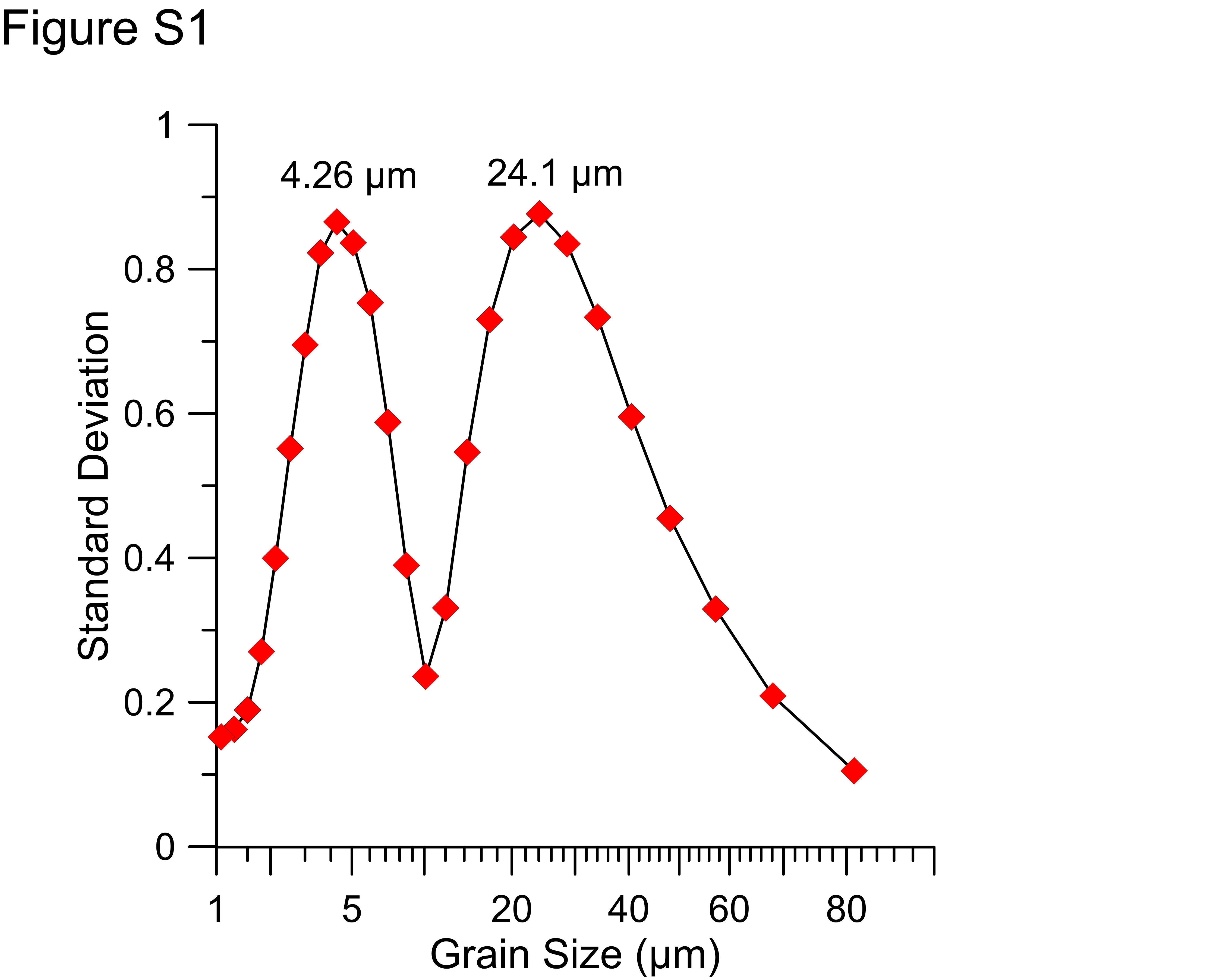
The grain size versus standard deviation method was used to distinguish the different controlling factors of the sedimentary processes (Yi et al., Reference Yi, Yu, Ortiz, Xu, Chen, Ge, Hao, Yao, Shi and Peng2012; Hu et al., Reference Hu, Yang, Zhao, Yoshiki, Fan and Wang2012; Zhou et al., Reference Zhou, Sun, Huang, Cheng and Jia2012; Zheng et al., Reference Zheng, Li, Wan, Jiang, Kao and Cody2014) and to further reconstruct current evolution and/or climate change in geologic history. Standard deviations were calculated for each of the 26 grain-size classes identified by the particle-size analyzer. Two peaks with larger standard deviations than the adjacent grain-size classes (4.3 and 21.4 μm) were observed, which represent the most sensitive fractions in response to changes in the sedimentary environment and are interpreted to represent environmentally sensitive size classes (Supplementary Fig. S1). The first sensitive size class (2.8–6.6 μm, fine fraction) ranged from 22.9% to 50.5%, with a mean value of 31.7%, and the second (15.6–37.2 μm, coarse fraction) varied between 0.02% and 21.5%, with a mean value of 11.8%. Figure 3 shows that the contents of the coarse and fine fractions exhibit apparent fluctuations and almost opposite trends along the core. The proportional contribution of these sensitive fractions shows a three-stage evolution, and the boundary is consistent with the grain-size division (Fig. 3a). The coarse fraction exhibited stable (9.5–7.1 ka), decreasing (7.1–1.6 ka), and increasing (1.6 ka to the present) trends over the past 9.5 ka (Fig. 3b). In contrast, the fine fraction demonstrated the opposite variation tendency (Fig. 3d). We calculated the mean grain-size range of the two components (Fig. 3c and e), in which the mean grain size of the fine fraction ranged from 4.3 to 4.6 μm and that of the coarse fraction ranged from 17.0 to 23.2 μm. The comparison between the mean grain size of the fine fraction samples and that of the coarse fraction shows that the mean grain size of sediment core YS01 was caused by the coarse fraction (Fig. 3a, c, and e), suggesting that fine fraction variation was passively caused by coarse fraction. Therefore, we considered that the coarse fraction was the environmentally sensitive grain-size fraction in core YS01.

Figure 3. (color online) Variations in the environmental proxies recorded in core YS01. (a) Mz (μm) mean grain size, which indicates the concentration trend of grain-size distribution. (b, d) Sensitive fractions (%). (c, e) Mean grain size for sensitive fraction (μm). (f) ${\rm U}{{K^{\prime}} \over {37}}$ -based sea-surface temperatures (SSTs) calibrated with the equation described in Müller et al. (Reference Müller, Kirst and Ruhland1998).
SST
The calibrated SST of core YS01 is shown in Fig. 3f and ranges from 12.5°C to 17.5°C with a mean value of 15.1°C throughout the past 9.5 ka (Jia et al., Reference Jia, Li, Yu, Zhao, Xiang, Li, Zhang and Zhao2019). The SST recorded in the SYS during the Holocene exhibited a distinct drop and rise at 5.6 and 2.6 ka, with temperatures of 2.9°C to 3.5°C, respectively. Based on the characteristics of SST distribution, the sedimentary environment of the SYS during the Holocene revealed by the core can be divided into five intervals, with boundaries at 7.0, 5.6, 2.6, and 1.2 ka (Fig. 3f). These are the warming, warm and stable, cold and stable, cooling, and warm and stable periods from the early Holocene to the present. The SST of the SYS fluctuated frequently during the Holocene and did not moderate until 2.6 ka. Interestingly, the sediments of the core regularly recorded several cooling events, including the periods of 8.8–8.5, 8.3–7.9, 7.6–7.3, 7.1–6.7, 6.4–6.1, 5.6–5.2, 5.1–4.8, 4.3–4.0, 3.4–3.1, 2.9–2.6, and 1.6–1.2 ka (Fig. 3f). The largest cooling amplitude was up to ~4.5°C at approximately 6.9 ka.
Clay minerals
The relative abundances of four minerals—smectite, illite, chlorite, and kaolinite—were plotted together with the illite chemistry index for the core (Fig. 4). The assemblages are mainly composed of illite (55.0%–66.5%, average 61.9%), followed by chlorite (10.1%–17.4%, average14.2%), kaolinite (6.8%–13.7%, average 9.7%), and smectite (10.2%–21.0%, average14.2%). The illite chemical index varies between 0.36 and 0.62, with an average of 0.5. In general, the down-core variations of clay minerals in core YS01 display a two-step mode divided by 6.7 m (5.0 ka). Smectite and illite have an inverse trend, with low smectite and high illite at 6.7–1.2 m and high smectite and low illite at 10.8–6.7 m. Chlorite shows a trend similar to illite, whereas kaolinite shows no obvious trend (Fig. 4).

Figure 4. (color online) Downcore variation of clay mineral assemblages (a–d), illite chemistry index (e), and illite/chlorite ratio (f).
DISCUSSION
Potential sources of clay mineral
Previous studies have suggested that the detrital sediments in the SYS are mainly derived from the Huanghe, Yangtze River, and surrounding small rivers in Korea (Yang and Youn, Reference Yang and Youn2007). The clay minerals in the sediments of surrounding rivers have been well studied (Table 2). Huanghe sediments show relatively high smectite content (>10%), while Yangtze River sediments contain relatively more illite plus chlorite content (Yang et al., Reference Yang, Jung, Lim and Li2003; Xu et al., Reference Xu, Lim, Choi, Yang and Jung2009b; Choi et al., Reference Choi, Lim, Park, Kim, Kang and Jung2010; Cho et al., Reference Cho, Kim, Kwak, Choi and Khim2015; Lu et al., Reference Lu, Li, Huang and Li2015; Zhang et al., Reference Zhang, Wan, Clift, Huang, Yu, Zhang and Mei2019a) and less smectite (<10%) compared with Huanghe sediments. More chlorite (>20%) and less kaolinite content (<5%) in Yalujiang sediments (Li et al., Reference Li, Hu, Wei, Zhao, Zou, Bai, Dou, Wang and Fang2014b) and more kaolinite (15%) and less smectite (<5%) content are found in Korean rivers sediments (Yang et al., Reference Yang, Jung, Lim and Li2003; Cho et al., Reference Cho, Kim, Kwak, Choi and Khim2015). Due to the high smectite content in the Huanghe sediments in comparison with other possible sources, the smectite/illite ratio can be used to distinguish the Huanghe source (Li et al., Reference Li, Hu, Wei, Zhao, Zou, Bai, Dou, Wang and Fang2014b). In addition, chlorite is usually produced by metamorphic rocks in high latitudes through physical weathering, while kaolinite is formed in warm-humid environments and is the product of chemical weathering. Therefore, the kaolinite/chlorite ratio can be used to reflect the variation in climate and identify the source area (Li et al., Reference Li, Hu, Wei, Zhao, Zou, Bai, Dou, Wang and Fang2014b). Furthermore, the clay minerals in the mud deposits off the southern Shandong Peninsula and modern Yangtze River delta during the Holocene have similar compositions to the modern Huanghe and Yangtze River fluvial sediments, respectively (Liu et al., Reference Liu, Saito, Wang, Yang and Nakashima2007; Wang and Yang, Reference Wang and Yang2013). This means that no significant changes have taken place in the clay mineral compositions of the Huanghe and Yangtze River sediments during the Holocene.
Table 2. Comparison of clay mineral assemblage between core YS01 and potential provenances.

A ternary diagram of smectite-(kaolinite+chlorite)-illite and a discrimination plot of smectite/illite versus kaolinite/chlorite ratios were produced to discern the provenance of clay minerals of core YS01 (Fig. 5). These plots show that most of the core sediments are scattered on the Huanghe source, indicating that they may have predominantly originated from the Huanghe during the Holocene (Fig. 5). The influence of Yangtze River and Korean rivers sediments is limited. Based on the studies of clay minerals in these sediments by Fan et al. (Reference Fan, Yang, Mao and Guo2001), the illite/smectite ratio in the core sediments ranges from 2.7 to 6.4, which further supports these results. The sediments derived from Korean rivers were mostly deposited along the Korean Peninsula, and the sediments that reached the core can be ignored due to the low suspended material from these rivers (Yang et al., Reference Yang, Jung, Lim and Li2003). Therefore, the decrease of the smectite/illite ratio at 5.0 ka can be attributed to the mixing of sediments from the Yangtze River, which further reveals that the YSWC intruded into the study area during this period. Previous studies have also suggested that the inflow of the YSWC started at 6.4–4.3 ka (Kong et al., Reference Kong, Park, Han, Chang and Mackensen2006; Xiang et al., Reference Xiang, Yang, Saito, Fan, Chen, Guo and Chen2008; Li et al., Reference Li, Nan, Jiang, Sun, Zhang and Li2009).

Figure 5. (color online) Ternary diagram (a) and discrimination plot (b) showing the variation in clay mineral assemblages of core YS01 from the South Yellow Sea. The clay mineral data of the potential sources are also plotted for comparison.
Paleoclimatic interpretations of the proxies: grain size and SST
Grain-size fractions sensitive to the sedimentary environment
Sensitive fraction is one of the proxies that can record changes in the sedimentary environment directly and has been widely used for the reconstruction of paleoenvironmental evolution (Xiao et al., Reference Xiao, Li, Liu, Chen, Xie, Jiang, Li, Xiang and Chen2006; Zheng et al., Reference Zheng, Li, Wan, Jiang, Kao and Cody2014; Kang et al., Reference Kang, Wang, Roberts, Duller, Cheng, Lu and An2018; Zhou et al., Reference Zhou, Liu, Yan, Zhang, Yi, Yang and Xiang2019). Coarse fractions in the muddy sediments of the eastern China Sea have generally been considered to be related to the enhancement of the coastal current and are considered to reflect winter monsoon intensity (Xiao et al., Reference Xiao, Li, Liu, Chen, Xie, Jiang, Li, Xiang and Chen2006; Hu et al., Reference Hu, Yang, Zhao, Yoshiki, Fan and Wang2012). However, coarse fractions are also affected by summer monsoon precipitation and typhoons related to river runoff and the in situ resuspension of sediments, respectively (Yang and Chen, Reference Yang and Chen2007; Yi et al., Reference Yi, Yu, Ortiz, Xu, Chen, Ge, Hao, Yao, Shi and Peng2012; Zhou et al., Reference Zhou, Sun, Huang, Cheng and Jia2012; Tian et al., Reference Tian, Fan, Zhang, Chen, Wang, Liu and Yang2019; Zhou et al., Reference Zhou, Liu, Yan, Zhang, Yi, Yang and Xiang2019). In general, the geologic implications of the coarse fraction of sediment in the muddy area need to be analyzed based on the characteristics of the study area itself.
The provenance result mentioned in the previous section shows that the sediments in core YS01 were derived from the Huanghe during the Holocene. Frequency distribution curves exhibit unimodal distribution characteristics and the content of each component in the sediment shows no significant changes (Fig. 2d, e, and f), indicating a stable hydrodynamic environment. Furthermore, high water content with almost nonexistent fine sand and very low coarse silt content indicate that sedimentary deposits occur in marine environments with weak hydrodynamics (Zhou et al., Reference Zhou, Dong and Li2015). It is well known that strong wave action induced by winter gales causes the resuspension of coastal sediments, and these sediments can be transported to the central SYS through the coastal currents with greater transport distances in winter (Bian et al., Reference Bian, Jiang and Greatbatch2013; Gao et al., Reference Gao, Qiao and Li2016). The grain-size analysis shows that fine fractions account for a large proportion of the sediment (Fig. 3d) and are closely related to the coastal current driven by the winter monsoon. However, considering the small contribution of this fraction to the change of sediment grain size (Fig. 3e), we considered that the coastal current is not the main factor controlling the change of sediment grain size in the study area. The coarse fractions with poor sorting may represent event deposition.
A strong typhoon in summer is the most likely factor causing the change of the sedimentary dynamic environment in the study area. Sediment records show that the grain size of the resuspended sediment affected by typhoons is coarser than that of normal sediments (Tian et al., Reference Tian, Fan, Zhang, Chen, Wang, Liu and Yang2019; Zhou et al., Reference Zhou, Liu, Yan, Zhang, Yi, Yang and Xiang2019). Observation data of suspension in the SYS show that the suspension concentration near the seabed following typhoon transit in summer is much higher than in winter (Gao et al., Reference Gao, Qiao and Li2016). Thus, the influence of a typhoon on the sedimentary process is very important. The storm wave reaches and disturbs the local sediment and the resuspended coarse sediments, with poor sorting redeposition in situ. The distribution characteristics of grain-size parameters also show that sediment sorting becomes poor with an increase in the coarse fraction (Figs. 2 and 3). According to our statistics of typhoons in the past 70 yr, approximately two summer typhoons occur in the SYS every year on average. Therefore, typhoons can be regarded as the main factor affecting coarse fraction in the muddy area of the SYS. The content and mean grain size of coarse fractions reflect the frequency and intensity of the typhoon, respectively. Generally, a typhoon will occur during the prevailing summer monsoon period, and its intensity increases during relatively warm periods (Bender et al., Reference Bender, Knutson, Tuleya, Sirutis, Vecchi, Garner and Held2010; Knutson et al., Reference Knutson, Sirutis, Zhao, Tuleya, Bender, Vecchi, Villarini and Chavas2015; Zhou et al., Reference Zhou, Liu, Yan, Zhang, Yi, Yang and Xiang2019). Therefore, the coarse fraction in the study area can be used to reflect the intensity of the storm, and the EASM can then be reconstructed.
SST
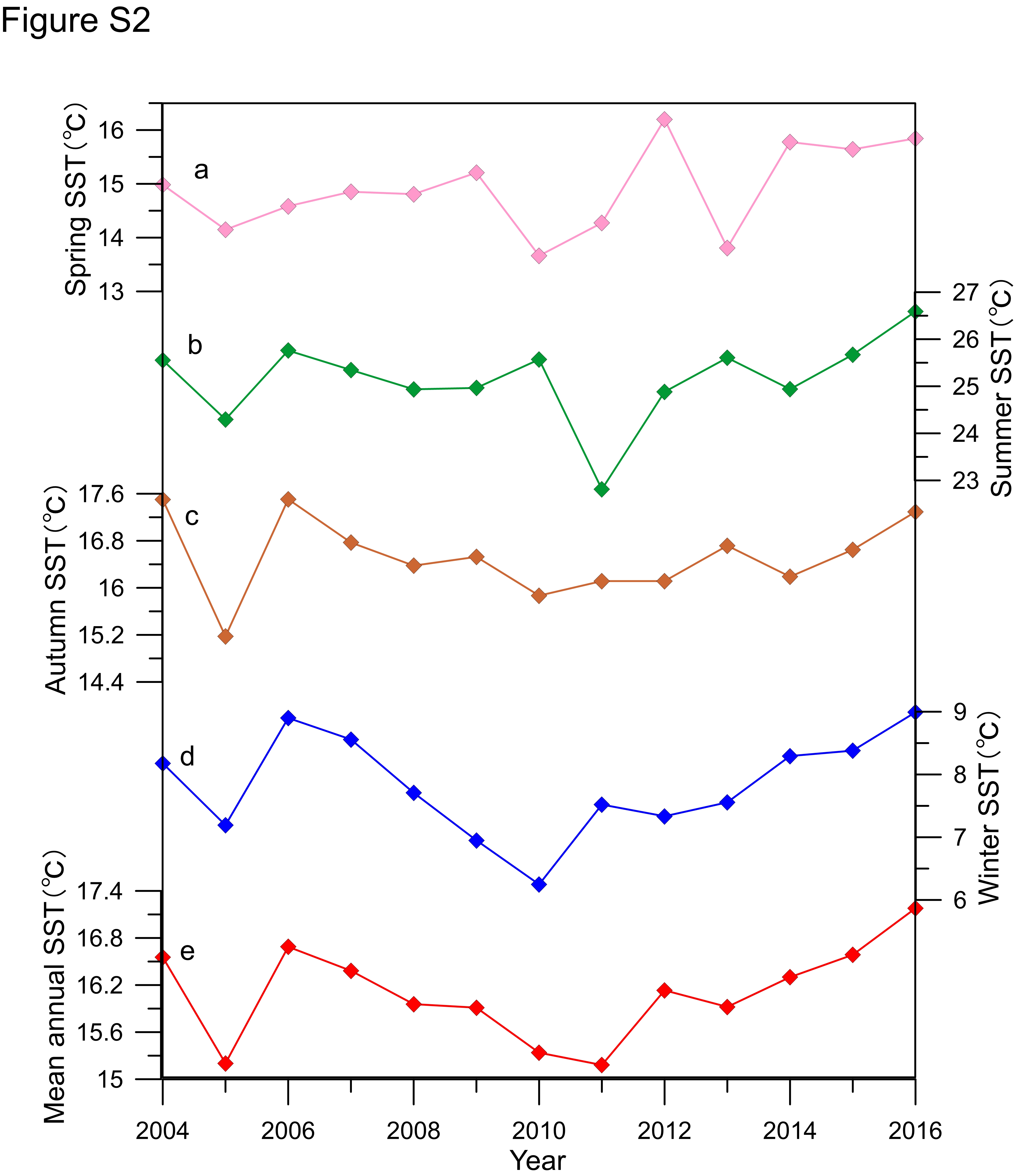
SST in summer and winter changes from 22.8°C to 26.6°C and from 6.2°C to 9.0°C, respectively; annual mean SST varies from 15.2°C to 17.2°C (Supplementary Fig. S2). The SST reconstructed by the core, ranging from 12.5°C to 17.5°C, is close to the annual mean SST. A positive correlation between surface sediment ${\rm U}{{K^{\prime}} \over {37}}$ values and mean annual SSTs in the Yellow Sea has also been found (Tao et al., Reference Tao, Xing, Luo, Wei, Liu and Zhao2012; Ruan et al., Reference Ruan, Xu, Ding, Wang and Zhang2015; Jia et al., Reference Jia, Li, Yu, Zhao, Xiang, Li, Zhang and Zhao2019); therefore, we interpreted ${\rm U}{{K^{\prime}} \over {37}}$
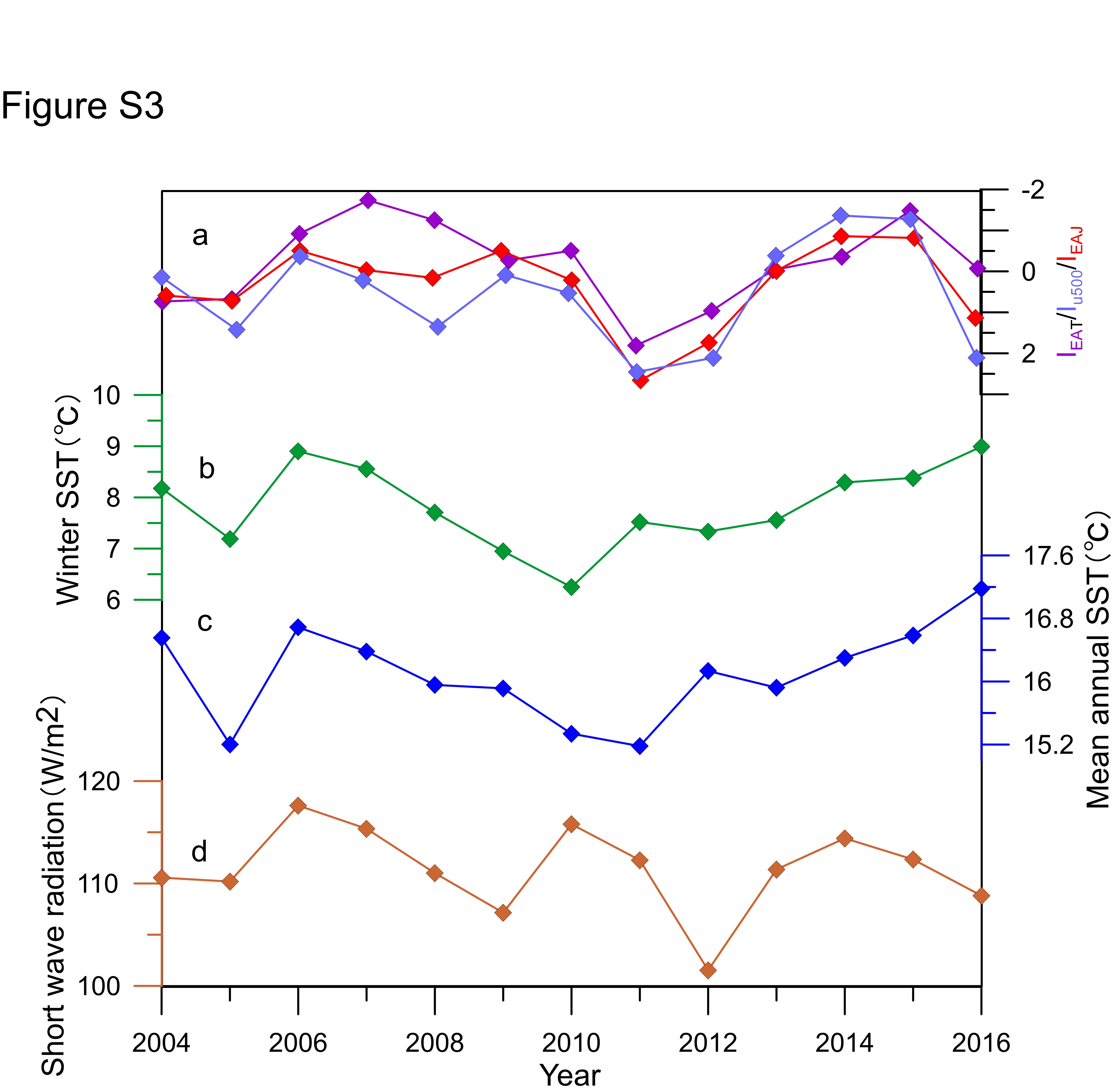
 -derived SST as annual mean SST in the study site. We compared seasonal and annual SSTs, and the result shows that annual SST has the same change trend as winter SST (Supplementary Fig. S2). Moreover, the SST variation characteristics of the eastern China Sea simulated by Zhang et al. (Reference Zhang, Zhou, He, Jiang, Liu, Xie, Sun and Liu2019b) show that the spatial distribution characteristics of annual mean SST depend on the variation of winter SST. Thus, the variations of SST reconstructed in this study can reflect SST changes in winter. The YSWC, as the only external heat source in the eastern China Sea, contributes to the variation in heat content in the SYS. The heat transported by the YSWC in winter is five times smaller than that of the net surface heat loss integrated over the Yellow Sea (Wei et al., Reference Wei, Yuan, Lu, Zhang and Luo2013). The winter SST is inversely and weakly correlated with the EAWM indices and short-wave radiation, respectively (Supplementary Fig. S3), indicating that the EAWM—rather than short-wave radiation—controls SST in the Yellow Sea. Therefore, the SST can be used to reconstruct the evolution of the EAWM. For the paleoclimate records that lack instrumental data, we assume that the mechanism of SST variation is also applicable.
Inference of the EAM intensity over the last ~9.5 ka
In-phase variations in EAWM and EASM intensity on orbital time scale
Variation in the intensity of the EASM and EAWM in the SYS during the Holocene were reconstructed based on the sedimentary records revealed by core YS01. The EASM can be divided into three periods: strong and relatively stable during 9.5–7.0 ka, weakened during 7.0–1.5 ka, and enhanced during 1.5–0 ka (Fig. 3c). Variations in coarser fractions in core YS01 present a gradual decrease from 25% to 9%, indicating that the EASM had a weakening trend over the past 9.5 ka. This weakening trend on the orbital time scale is also well documented by δ18O values from stalagmites (Wang et al., Reference Wang, Cheng, Edwards, He, Kong, An, Wu, Kelly, Dykoski and Li2005; Fig. 6d) and pollen from lake sediments (Shen et al., Reference Shen, Liu, Wang and Matsumoto2005; Chen et al., Reference Chen, Xu, Chen, Birks, Liu, Zhang and Jin2015). On the other hand, the SSTs record a distinct drop at 5.6 ka with a range of 2.9°C, which represents the sudden strengthening of the EAWM. Similarly, two distinct rising processes are found at 2.6 ka (3.5°C) and 1.2 ka (2.0°C), suggesting a rapid weakening of the EAWM. In general, SST records exhibit a linear rising trend overall (Fig. 7g), indicating a weakening of the EAWM on the orbital time scale. It also indicates that the EAWM can be divided into five periods at the millennial time scale: weakened conditions during 9.5–6.7 ka, weak and relatively stable conditions during 6.7–5.6 ka, strong and relatively stable conditions during 5.6–2.6 ka, enhanced conditions during 2.6–1.5 ka, and weak and stable conditions from 1.5 ka to the present (Fig. 3f). Winter monsoon proxy records, based on sedimentary records such as grain size obtained from Chinese loess and marine sediments (Stevens et al., Reference Stevens, Thomas, Armitage, Lunn and Lu2007; Hu et al., Reference Hu, Yang, Zhao, Yoshiki, Fan and Wang2012), temperature in the western Pacific (Steinke et al., Reference Steinke, Mohtadi, Groeneveld, Lin, Löwemark, Chen and Rendle-Bühring2010, Reference Steinke, Glatz, Mohtadi, Groeneveld, Li and Jian2011; Huang et al., Reference Huang, Tian and Steinke2011), and dust flux in the eastern Tibetan Plateau (Yu et al., Reference Yu, Zhou, Liu and Kang2011) revealed the same linear weakening characteristics of the winter monsoon on an orbital time scale during the Holocene. Consequently, the results in this study reveal in-phase changes between summer and winter monsoons in the SYS on orbital time scales (Figs. 6 and 7).

Figure 6. (color online) East Asian summer monsoon (EASM) variations on the orbital time scale during the Holocene. (a) Summer insolation at 35°N, W/m2(Laskar et al., Reference Laskar, Robutel, Joutel, Gastineau, Correia and Levrard2004). (b) EASM wind index in TRACE21 (Wen et al., Reference Wen, Liu, Wang, Cheng and Zhu2016); JJA, the simulated meridional wind speed in June-July-August. (c) Variations in the content of the coarser grain-size component (this study). (d) δ18O variability in stalagmites from the Dongge Cave (China; Wang et al., Reference Wang, Cheng, Edwards, He, Kong, An, Wu, Kelly, Dykoski and Li2005). (e) Summer monsoon index derived from Qinghai Lake (An et al., Reference An, Colman, Zhou, Li, Brown, Timothy Jull and Cai2012); SMI, Summer monsoon index. (f) Bulk Ti content from Cariaco basin sediments from Ocean Drilling Project (ODP) Site 1002 (Haug et al., Reference Haug, Hughen, Sigman, Peterson and Röjl2001), which represents the Intertropical Convergence Zone (ITCZ) shift.

Figure 7. (color online) East Asian winter monsoon (EAWM) variations on the orbital time scale during the Holocene. (a) Winter insolation at 35°N and 65°N, W/m2(Laskar et al., Reference Laskar, Robutel, Joutel, Gastineau, Correia and Levrard2004). (b) Lake Qinghai westerlies climate index (WI; flux of >25 μm fraction; An et al., Reference An, Colman, Zhou, Li, Brown, Timothy Jull and Cai2012). (c) Gaussian smoothed (200 yr) GISP2 potassium (K+; ppb) ion proxy for the Siberian High (Mayewski et al., Reference Mayewski, Rohling, Stager, Karlén, Maasch, Meeker, Meyerson and Gasse2004). (d) EAWM wind index in TRACE21 (Wen et al., Reference Wen, Liu, Wang, Cheng and Zhu2016); DJF, December-January-February. (e) The δ18O record from core SK-2 in the western North Pacific (Sagawa et al., Reference Sagawa, Kuwae, Tsuruoka, Nakamura, Ikehara and Murayama2014). (f) Sea-surface temperature (SST) gradient between the surface and thermocline waters in the South China Sea, core MD05-2904 (Steinke et al., Reference Steinke, Glatz, Mohtadi, Groeneveld, Li and Jian2011), and the west–east SST gradient between the southwestern and southeastern SST stacks (Huang et al., Reference Huang, Tian and Steinke2011). (g) ${\rm U}{{K^{\prime}} \over {37}}\;$ -reconstructed SST in core YS01 (this study).
The near linear trend of the EAWM and EASM may be related to the seasonal insolation triggered by orbital elements at orbital time scales during the Holocene (Figs. 6 and 7). Wen et al. (Reference Wen, Liu, Wang, Cheng and Zhu2016) conducted a long-term transient simulation of climate evolution forced by orbital forcing individually, and a positive correlation between the EAWM and the EASM at orbital time scales was found (Figs. 6b and 7d). Enhanced (decreased) winter (summer) solar insolation in the Northern Hemisphere corresponds to weakening winter (summer) monsoons. As shown in Figure 7c, there is a decreasing trend in the K+ derived from core GISP2 (Mayewski et al., Reference Mayewski, Rohling, Stager, Karlén, Maasch, Meeker, Meyerson and Gasse2004), which indicates a weakening of the Siberian High during the Holocene (Lorenz et al., Reference Lorenz, Kim, Rimbu, Schneider and Lohmann2006). The intensity of westerlies during the Holocene did not show a linear trend similar to the EAWM variations (Fig. 7b), indicating that the meridional temperature gradient in the Northern Hemisphere is relatively stable on orbital time scales (An et al., Reference An, Colman, Zhou, Li, Brown, Timothy Jull and Cai2012). The AMOC developed steadily during the Holocene (McManus et al., Reference McManus, Francois, Gherardi, Keigwin and Brown-Leger2004); therefore, the North Atlantic cold signal has no significant effect on the winter monsoon at this time scale. The increase in the winter insolation leads to winter warming in eastern Siberia (Lorenz et al., Reference Lorenz, Kim, Rimbu, Schneider and Lohmann2006), which suppresses the development of the Siberian High (Sagawa et al., Reference Sagawa, Kuwae, Tsuruoka, Nakamura, Ikehara and Murayama2014). The decrease in the thermal difference from land to sea caused by the weakening of the Siberian High is the most likely factor causing the weakening of the EAWM. On the other hand, decreased solar insolation in the Northern Hemisphere in summer leads to a decrease in the thermal difference from sea to land, which directly results in the weakening of the summer monsoon (Dykoski et al., Reference Dykoski, Edwards, Cheng, Yuan, Cai, Zhang, Lin, Qing, An and Revenaugh2005; Shen et al., Reference Shen, Liu, Wang and Matsumoto2005; Wang et al., Reference Wang, Cheng, Edwards, He, Kong, An, Wu, Kelly, Dykoski and Li2005; An et al., Reference An, Colman, Zhou, Li, Brown, Timothy Jull and Cai2012; Chen et al., Reference Chen, Xu, Chen, Birks, Liu, Zhang and Jin2015; Wen et al., Reference Wen, Liu, Wang, Cheng and Zhu2016). Meanwhile, the ITCZ migrates southward with decreasing monsoon precipitation (Fig. 6f; Haug et al., Reference Haug, Hughen, Sigman, Peterson and Röjl2001; Poore et al., Reference Poore, Quinn and Verardo2004), which is another response of the internal atmospheric circulation of the Earth to the weakening of summer insolation.
In general, it is understood that the EASM and EAWM are positively correlated over orbital time scales in the SYS during the Holocene. Moreover, considering that the EAM originates from the thermal difference between land and sea (Hu et al., Reference Hu, Yang, Zhao, Yoshiki, Fan and Wang2012), the seasonal variation of solar insolation is the first-order control factor. The orbital-driven solar insolation is the fundamental reason for the weakening of the EAWM and EASM on orbital time scales. This is different from the previous understanding that an inverse phase change of the EAWM and EASM is driven by the variation in summer solar insolation intensity at high latitudes in the Northern Hemisphere. In fact, they are controlled by relatively independent systems and show in-phase changes on the orbital scale during the Holocene.
Out-of-phase variations in EAWM and EASM on centennial time scale
The sediment record shows centennial-scale variability superimposed on the long-term trend during the Holocene (Fig. 3b and f). Previous studies have proposed that the relationship between winter and summer monsoons in East Asia was spatially and temporally variable on a centennial time scale (Wang et al., Reference Wang, Li, Lu, Gu, Rioual, Hao and Mackay2012; Kang et al., Reference Kang, Wang, Roberts, Duller, Cheng, Lu and An2018). To reveal the evolution of the monsoon on centennial/multicentennial time scales in the SYS, the original paleoclimate data had to be smoothed and detrended. The 1000 and 200 yr moving averages were applied to the coarse fraction and SST to obtain millennial- and centennial-scale monsoon changes. This method has been widely used in paleoclimate research (Sagawa et al., Reference Sagawa, Kuwae, Tsuruoka, Nakamura, Ikehara and Murayama2014; Hao et al., Reference Hao, Liu, Ogg, Liang, Xiang, Zhang, Zhang, Zhang, Liu and Li2017; Kang et al., Reference Kang, Wang, Roberts, Duller, Cheng, Lu and An2018). The same method was applied to other climate indicators collected, such as the westerlies index (WI), the Siberian High (SH), and the total solar irradiance (TSI), among others. To find centennial-scale variability, low-frequency millennial-scale variability must be removed by subtracting the 1000 yr moving average. Anomalies in the centennial-scale variability are standardized using the standard deviation, following Sagawa et al. (Reference Sagawa, Kuwae, Tsuruoka, Nakamura, Ikehara and Murayama2014).
The winter monsoon revealed in the SYS is consistent with that reconstructed using SST during the winter season in the western North Pacific and is within the dating error (Sagawa et al., Reference Sagawa, Kuwae, Tsuruoka, Nakamura, Ikehara and Murayama2014; Fig. 8d and e). Similarly, variability in the coarse fraction in the study area and the δ18O records of stalagmites in Dongge Cave show a good correlation on centennial time scales (Wang et al., Reference Wang, Cheng, Edwards, He, Kong, An, Wu, Kelly, Dykoski and Li2005; Fig. 8g and h). These characteristics further explain the reliability of the reconstruction of the EAM evolution in this study. An inverse relationship between the summer and winter monsoons on centennial scales was found (Fig. 8e and g), which is similar to the periods during the Younger Dryas, Heinrich, and ~8.2 ka cooling event. To investigate the factors that drive the EAM changes on centennial time scales, the detrended global paleoclimatic indicators (e.g., the TSI, North Atlantic IRD, SH, WI, and ITCZ) and the EAM reconstructed in this study were selected for spectral analysis. The results show that all indicators show a significant ~700-yr-cycle period, and the confidence level of this period is more than 99% (Fig. 9), indicating an inherent connection between these indicators on the centennial time scale.

Figure 8. (color online) Centennial time scale variations in paleoclimatic indicators. (a) The westerlies index (WI; flux of >25 μm fraction) record (An et al., Reference An, Colman, Zhou, Li, Brown, Timothy Jull and Cai2012). (b) The standardized record of GISP2 potassium (K+; ppb) ions, which can be used to reconstruct the Siberian High (SH; Mayewski et al., Reference Mayewski, Rohling, Stager, Karlén, Maasch, Meeker, Meyerson and Gasse2004). (c) The standardized record of drift ice for MC52-VM29-191 during the Holocene (Bond et al., Reference Bond, Kromer, Beer, Muscheler, Evans, Showers, Hoffmann, Lotti-Bond, Hajdas and Bonani2001); HSG, Hematite-stained grains. (d) The standardized SK-2 δ18O record (Sagawa et al., Reference Sagawa, Kuwae, Tsuruoka, Nakamura, Ikehara and Murayama2014). (e) The standardized record of ${\rm U}{{K^{\prime}} \over {37}}$ - reconstructed sea-surface temperature (SST) in the YS01 core (this study). (f) The standardized record of the total solar irradiance (TSI; Steinhilber et al., Reference Steinhilber, Beer and Frohlich2009). (g) The standardized YS01 coarser grain-size component content (this study). (h) The standardized Dongge Cave δ18O record (Wang et al., Reference Wang, Cheng, Edwards, He, Kong, An, Wu, Kelly, Dykoski and Li2005). (i) The standardized record bulk Ti content from the Cariaco basin sediments from ODP Site 1002 (Haug et al., Reference Haug, Hughen, Sigman, Peterson and Röjl2001), which represents the shift of the Intertropical Convergence Zone (ITCZ). (j) The frequency of El Niño per 100 yr (Conroy et al., Reference Conroy, Overpeck, Cole, Shanahan and Steinitz-Kannan2008). Identical treatment of standardization, which includes the calculation of the 200 yr running mean anomaly from the 1000 yr running mean and its standardization using the standard deviation, is applied to the SST in the YS01 core, coarse-component content in the core, frequency of El Nino–Southern Oscillation (ENSO)/100 yr, flux of >25 μm fraction in sediment derived from Lake Qinghai, drift ice for the MC52-VM29-191 core, GISP2 potassium (K+; ppb) ions, bulk Ti content from the Cariaco basin sediments, and coarse component content in the core. Gray bars indicate significant cold periods in the YS01 record. EAWM, East Asian winter monsoon.

Figure 9. Spectral analysis results for paleoclimatic indicators. (a) Total solar irradiance (TSI; Steinhilber et al., Reference Steinhilber, Beer and Frohlich2009). (b) Ice-rafted debris (IRD; Bond et al., Reference Bond, Kromer, Beer, Muscheler, Evans, Showers, Hoffmann, Lotti-Bond, Hajdas and Bonani2001). (c) Siberian High (SH; Mayewski et al., Reference Mayewski, Rohling, Stager, Karlén, Maasch, Meeker, Meyerson and Gasse2004). (d) Westerlies index (WI; flux of >25 μm fraction) record (An et al., Reference An, Colman, Zhou, Li, Brown, Timothy Jull and Cai2012). (e) Sea-surface temperature (SST) in YS01 core (this study). (f) Sensitive coarse fraction (this study). (g) Bulk Ti content from the Cariaco basin sediments from ODP Site 1002 (Haug et al., Reference Haug, Hughen, Sigman, Peterson and Röjl2001). (h) The Dongge Cave δ18O record (Wang et al., Reference Wang, Cheng, Edwards, He, Kong, An, Wu, Kelly, Dykoski and Li2005). All data were interpolated at 10 yr intervals and analyzed using Redfit v. 3.8 software. The red and blue lines indicate the 99% and 95% confidence levels, respectively. ITCZ, Intertropical Convergence Zone. (For interpretation of the references to color in this figure legend, the reader is referred to the web version of this article.)
High-frequency solar activity, as external forcing, significantly influences Earth's climate system (Bond et al., Reference Bond, Kromer, Beer, Muscheler, Evans, Showers, Hoffmann, Lotti-Bond, Hajdas and Bonani2001; Fleitmann et al., Reference Fleitmann, Burns, Mudelsee, Neff, Kramers, Mangini and Matter2003; Dykoski et al., Reference Dykoski, Edwards, Cheng, Yuan, Cai, Zhang, Lin, Qing, An and Revenaugh2005; Huang et al., Reference Huang, Tian and Steinke2011, Reference Huang, Zeng, Ye and Wei2019; Sagawa et al., Reference Sagawa, Kuwae, Tsuruoka, Nakamura, Ikehara and Murayama2014). As shown in Figure 8d–h, low TSI (weak solar activity) reconstructed from 10Be in ice cores (Steinhilber et al., Reference Steinhilber, Beer and Frohlich2009) shows good agreement with the weak EASM record and the strong EAWM revealed in this study. Solar perturbation is independent of Earth's orbital motion, and its variability superimposes on long-term changes in insolation, which also has an impact on the climate system (Xiao et al., Reference Xiao, Li, Liu, Chen, Xie, Jiang, Li, Xiang and Chen2006; Sagawa et al., Reference Sagawa, Kuwae, Tsuruoka, Nakamura, Ikehara and Murayama2014). Weakened solar activity reduces the amount of solar radiation and leads to a strong winter monsoon and a weak summer monsoon. Figure 8 shows that the EAM reconstructed from the SYS is mostly related to solar activity, indicating that the variation in solar activity could be the crucial factor affecting the EAM at centennial time scales. Mayewski et al. (Reference Mayewski, Rohling, Stager, Karlén, Maasch, Meeker, Meyerson and Gasse2004) collected ~50 globally distributed paleoclimate records and proposed that the rapid climate changes during the Holocene were mostly forced by solar activity.
To further investigate the relationship between the EAM and solar activity, wavelet power spectrum analysis was performed for the SST record, the coarse fraction from the core, and the TSI record (Supplementary Fig. S4). The Morlet wavelet was chosen for the continuous wavelet transform in this study. The TSI power spectrum shows significant cyclicity of ~210 (de Vries cycle), 700, 490, and 350 yr cycles (Supplementary Fig. S4a). The power spectrum of SST shows a cyclicity of 700, 540–450, 330, and 250 yr with a 95% confidence level (Supplementary Fig. S4b), and the grain-size analysis shows 540, 454, 380–340, and 200 yr cycles (Supplementary Fig. S4c). The spectra of TSI and SST share almost common cyclicities, and these cyclicities exhibit strong power during the Holocene.
Considering the interoperability of the global climate system on the centennial time scale, the EAM is bound to be controlled by additional factors. We compared the IRD recorded in the North Atlantic, the westerlies recorded from Qinghai Lake on the northern Tibetan Plateau (An et al., Reference An, Colman, Zhou, Li, Brown, Timothy Jull and Cai2012), the GISP2 K+ (ppb) ion proxy for the SH (Mayewski et al., Reference Mayewski, Rohling, Stager, Karlén, Maasch, Meeker, Meyerson and Gasse2004), and the bulk Ti content from the Cariaco basin for the ITCZ migration with the EAM records of this study and found that they are correlated within the dating error (Fig. 8). Previous studies have proposed that the evolution of the EAM is closely related to North Atlantic forcing through the westerlies (Huang et al., Reference Huang, Tian and Steinke2011; Sun et al., Reference Sun, Clemens, Morrill, Lin, Wang and An2011; Hao et al., Reference Hao, Liu, Ogg, Liang, Xiang, Zhang, Zhang, Zhang, Liu and Li2017; Jia et al., Reference Jia, Li, Yu, Zhao, Xiang, Li, Zhang and Zhao2019), which can contribute to the out-of-phase behavior between the EAWM and the EASM. The formation of North Atlantic Deep Water is inhibited by meltwater input, which weakens or even shuts down the AMOC (Dykoski et al., Reference Dykoski, Edwards, Cheng, Yuan, Cai, Zhang, Lin, Qing, An and Revenaugh2005; Wen et al., Reference Wen, Liu, Wang, Cheng and Zhu2016). This results in heat retention in low latitudes (Wu et al., Reference Wu, Li, Yang and Xie2008; Böhm et al., Reference Böhm, Lippold, Gutjahr, Frank, Blaser, Antz, Fohlmeister, Frank, Andersen and Deininger2015) and large-scale cooling in the North Atlantic (Thomas et al., Reference Thomas, Wolff, Mulvaney, Steffensen, Johnsen, Arrowsmith, White, Vaughn and Popp2007). In addition, the meridional temperature gradient increases in the Northern Hemisphere (Böhm et al., Reference Böhm, Lippold, Gutjahr, Frank, Blaser, Antz, Fohlmeister, Frank, Andersen and Deininger2015), leading to the enhancement of westerlies. The influence of this process on the climate of East Asia manifests as the increase in the winter monsoon and the decrease in the summer monsoon (Sun et al., Reference Sun, Clemens, Morrill, Lin, Wang and An2011; Yang et al., Reference Yang, Dong and Xiao2019). Long-term transient simulations of climate evolution forced by North Atlantic meltwater also show that the EAWM and EASM are inversely correlated during the period of Heinrich 1, the Younger Dryas, and the ~8.2 ka cooling event (Wen et al., Reference Wen, Liu, Wang, Cheng and Zhu2016). A series of climate shifts (IRD events) driven by solar output were discovered in the North Atlantic during the Holocene (Bond et al., Reference Bond, Kromer, Beer, Muscheler, Evans, Showers, Hoffmann, Lotti-Bond, Hajdas and Bonani2001). An et al. (Reference An, Colman, Zhou, Li, Brown, Timothy Jull and Cai2012) proposed that the westerlies was linked to northern high-latitude climate and it also show periodic change during the Holocene (Fig. 8a). In addition, the westerlies are considered as the link between the North Atlantic and the EAM system. However, current evidence can only show that North Atlantic forcing has an effect on the EAM system and that it mostly manifests in an extreme cooling period related to the weakening of the AMOC (Sun et al., Reference Sun, Clemens, Morrill, Lin, Wang and An2011). More evidence is needed regarding its impact on EAM periodic evolution during the Holocene at centennial time scales. Due to a lack of evidence for the regular changes in the AMOC and/or meltwater inputs throughout the entire Holocene, North Atlantic forcing probably cannot be regarded as the decisive factor driving EAM evolution in the Holocene.
Precipitation is generally used to indicate EASM variation (Wang et al., Reference Wang, Cheng, Edwards, He, Kong, An, Wu, Kelly, Dykoski and Li2005). Its intensity is closely related to the migration of the annual mean position of the ITCZ (Yancheva et al., Reference Yancheva, Nowaczyk, Mingram, Dulski, Schettler, Negendank, Liu, Sigman, Peterson and Haug2007), which is associated with solar activity (Poore et al., Reference Poore, Quinn and Verardo2004) and ocean thermohaline circulation (Broccoli et al., Reference Broccoli, Dahl and Stouffer2006). The relatively good correlation between the migration of the ITCZ and the TSI changes on the centennial time scale (Fig. 8h and i) reveals that the location change of the ITCZ was probably controlled by solar activity during the Holocene. EASM intensity revealed by the grain-size spectrum is similar to the significant periods of the TSI record, but solar activity weakens and the summer monsoon does not respond well in some periods (Fig. 8f and h), such as at 7.3 and 4.9 ka, indicating that the variation of EASM strength on centennial time scales during the Holocene was regulated by other factors in addition to solar activity. That the EASM is not driven simply by changing solar insolation has also been revealed by speleothem isotope records (Wang et al., Reference Wang, Cheng, Edwards, He, Kong, An, Wu, Kelly, Dykoski and Li2005). The most significant summer monsoon weakening event occurred at 8.4–8.1 ka (Fig. 6g–i). It is considered the response of the SYS to the ~8.2 ka cooling event, is characterized by a cold and/or dry climate (Bond et al., Reference Bond, Kromer, Beer, Muscheler, Evans, Showers, Hoffmann, Lotti-Bond, Hajdas and Bonani2001; Hoffman and Jeremy, Reference Hoffman, Carlson, Winsor, Klinkhammer, LeGrande, Andrews and Strasser2012), and resulted from the meltwater outflow from the Laurentide ice margin lake to Hudson Bay (Carlson et al., Reference Carlson, Legrande, Oppo, Came, Schmidt, Anslow, Licciardi and Obbink2008; Wanner et al., Reference Wanner, Solomina, Grosjean, Ritz and Markéta2011; Hoffman and Jeremy, Reference Hoffman, Carlson, Winsor, Klinkhammer, LeGrande, Andrews and Strasser2012). Eventually, it caused the Northern Hemisphere to cool and the ITCZ to migrate southward (Poore et al., Reference Poore, Quinn and Verardo2004) and a weakening of the EASM (Broccoli et al., Reference Broccoli, Dahl and Stouffer2006; Yu et al., Reference Yu, Gao, Wang, Guo and Li2009).
In recent years, it has been proposed that the EAM is driven by the ENSO (Jia et al., Reference Jia, Bai, Yang, Xie, Wei, Ouyang, Chu, Liu and Peng2015; Park et al., Reference Park, Shin and Byrne2016; Li et al., Reference Li, Zhao and Tian2017; Huang et al., Reference Huang, Zeng, Ye and Wei2019; Zhao et al., Reference Zhao, Wan, Song, Gong, Zhai, Shi and Li2019). However, the frequency of the ENSO per 100 yr during the Holocene has only increased since the late Holocene (Conroy et al., Reference Conroy, Overpeck, Cole, Shanahan and Steinitz-Kannan2008). Its weak correlation with the EAM also suggests that ENSO activity is not the decisive factor for the periodic change of the EAM during the Holocene (Fig. 8j). In general, internal forcing is not the decisive factor controlling the periodic changes of the EAM on the centennial time scale, even though the ENSO, ITCZ, and North Atlantic forcing all contribute to EAM evolution. Therefore, the ~700 yr periodic evolution of the EAM reconstructed in the SYS is mainly controlled by solar activity.
CONCLUSIONS
A high-resolution core (YS01) retrieved from the central muddy area in the SYS was analyzed for grain size, U${{K^{\prime}} \over {37}}$ -based SST, and clay mineral assemblages to investigate the source of clay minerals and reconstruct the evolution of the EAM for the past 9500 years. The clay mineral assemblages for the core mainly consist of illite (61.9%), followed by chlorite (14.2%), smectite (average 14.2%), and kaolinite (average 9.7%). In addition, the illite/smectite ratio in core sediments ranges from 2.7 to 6.4, indicating a Huanghe source in the study area. The coarse fraction and SST were used to reconstruct the evolution of the EASM and the EAWM, respectively. The EASM is manifested in the following three variations: strong and relatively stable during 9.5–7.0 ka, weakened during 7.0–1.5 ka, and strengthened during 1.5–0 ka. Similarly, the EAWM can be divided into five stages: weakened during 9.5–6.7 ka, weak and relatively stable during 6.7–5.6 ka, strong and relatively stable during 5.6–2.6 ka, strengthened during 2.6–1.5 ka, and weak and stable from 1.5 ka to the present. We also found that the EASM and EAWM are correlated at the orbital time scale in response to orbital-driven solar insolation forcing, but anticorrelated at centennial time scales in terms of solar activity.
ACKNOWLEDGMENTS
This study was jointly funded by the National Natural Science Foundation of China (grant nos. 41030856 and 41606216) and the Taishan Scholar Project grant to GL. Our heartfelt thanks to all the expedition staff and crew who took part in the field drilling the borehole core YS01. Constructive and valuable comments from senior editor Derek Booth, associate editor Kathleen Johnson, and other three anonymous reviewers are greatly appreciated. We also thank them for improving the English.
SUPPLEMENTARY MATERIAL
The supplementary material for this article can be found at https://doi.org/10.1017/qua.2020.62