INTRODUCTION
Insight into how individual species respond to resources in tree communities is critical for understanding how environmental factors influence the distribution, abundance and coexistence of tropical tree species (Condit et al. Reference CONDIT, ENGELBRECHT, PINO, PÉREZ and TURNER2013). At a large scale, rainfall has been shown to influence species richness (ter Steege et al. Reference TER STEEGE, PITMAN, PHILLIPS, CHAVE, SABATIER, DUQUE, MOLINO, PRÉVOST, SPICHIGER and CASTELLANOS2006), composition (Hall & Swaine Reference HALL and SWAINE1976) and distribution (Bongers et al. Reference BONGERS, POORTER, VAN ROMPAEY and PARREN1999, Engelbrecht et al. Reference ENGELBRECHT, COMITA, CONDIT, KURSAR, TYREE, TURNER and HUBBELL2007, Swaine Reference SWAINE1996, Toledo et al. Reference TOLEDO, PEÑA-CLAROS, BONGERS, ALARCÓN, BALCÁZAR, CHUVIÑA, LEAÑO, LICONA and POORTER2012), whereas at smaller scales soil fertility, topography and irradiance can affect species distribution (John et al. Reference JOHN, DALLING, HARMS, YAVITT, STALLARD, MIRABELLO, HUBBELL, VALENCIA, NAVARRETE and VALLEJO2007, Veenendaal et al. Reference VEENENDAAL, SWAINE, LECHA, WALSH, ABERBRESE and OWUSU-AFRIYIE1996). Most tropical forests show seasonal variation in rainfall, and species drought performance and physiological drought tolerance have therefore been found to determine the distribution of tropical species (Baltzer et al. Reference BALTZER, DAVIES, BUNYAVEJCHEWIN and NOOR2008, Engelbrecht et al. Reference ENGELBRECHT, COMITA, CONDIT, KURSAR, TYREE, TURNER and HUBBELL2007).
A number of studies (Hall & Swaine Reference HALL and SWAINE1976, John et al. Reference JOHN, DALLING, HARMS, YAVITT, STALLARD, MIRABELLO, HUBBELL, VALENCIA, NAVARRETE and VALLEJO2007, Toledo et al. Reference TOLEDO, PEÑA-CLAROS, BONGERS, ALARCÓN, BALCÁZAR, CHUVIÑA, LEAÑO, LICONA and POORTER2012) have used composite axes of multivariate environmental gradients and vegetation gradients to analyse species distribution, but the use of such axes does not give insight into how individual species respond to specific environmental factors (Condit et al. Reference CONDIT, ENGELBRECHT, PINO, PÉREZ and TURNER2013). For example, several species in Ghana (e.g. Khaya anthotheca and Pericopsis elata) do not follow the main vegetation gradient that parallels the annual rainfall gradient, and by inference may not follow the rainfall gradient (Hawthorne Reference HAWTHORNE1995). Studies that have evaluated the response of tropical tree species to individual environmental gradients have focused on soil nutrients, rainfall and water availability, but far less attention has been paid to the role of temperature. Seasonal variation in temperature is rather minor across most tropical forests, but recent studies suggest that small changes in temperature are likely to affect species distribution patterns (Wright Reference WRIGHT2010), although there are still few data to support this point. Determination of individual species response curves to a range of climatic variables is imperative to identify the climatic variables that are biologically most relevant to individual plant species, as they can help to predict the possible consequences of climate change for tropical forests (Borchert Reference BORCHERT1998).
Vegetation structure and composition vary continuously along environmental gradients and theoretical models assume that species show bell-shaped, symmetrical responses to gradients (Gauch & Whittaker Reference GAUCH and WHITTAKER1972) especially when the gradient is long such as the rainfall gradient in Ghana. However, there is growing evidence that many species show asymmetrical response curves to environmental gradients (e.g. Oksanen & Minchin Reference OKSANEN and MINCHIN2002).
In this study, we evaluated the distributions of 20 Ghanaian woody tree species that are economically important (for timber or non-timber products), have contrasting distributions within forest types and that differ in shade tolerance. We described species distributions using detailed inventory data from 2505 1-ha plots across a steep rainfall gradient (1100–2000 mm y−1) in Ghana. We determined the influence of annual rainfall, temperature and their seasonality on species presence/absence. The size of this study (2505 plots) is an order of magnitude larger than has been studied so far (e.g. 220 plots by Toledo et al. Reference TOLEDO, PEÑA-CLAROS, BONGERS, ALARCÓN, BALCÁZAR, CHUVIÑA, LEAÑO, LICONA and POORTER2012; 72 plots by Condit et al. Reference CONDIT, ENGELBRECHT, PINO, PÉREZ and TURNER2013). Two questions were addressed: First, what is the relative importance of annual rainfall, temperature and their seasonality for species distribution? We hypothesized that annual rainfall, and especially rainfall seasonality will be stronger drivers of species distribution than temperature (seasonality). Second, what is the shape of species response curves along these environmental gradients? We hypothesized that unimodal response curves will be more associated with rainfall gradient than temperature gradient because under relatively benign conditions environmental resources (such as water) are more important in shaping species responses than environmental conditions such as temperature.
MATERIALS AND METHODS
Study site
The study was based on Ghanaian national forest inventory data summarized by Hawthorne (Reference HAWTHORNE1995, Reference HAWTHORNE1996) and Hawthorne & Abu-Juam (Reference HAWTHORNE and ABU-JUAM1995). The study area was located between latitudes 4.7°–8.0°N and longitudes 3.2°E–0.6°W. Based on floristic composition, the forest vegetation of Ghana has been classified into seven main forest types: wet evergreen, moist evergreen, upland evergreen, moist semi-deciduous, dry semi-deciduous, southern marginal and south-east outlier forests (Hall & Swaine Reference HALL and SWAINE1976). The forests are characterized by a rainfall gradient which varies from < 750 to > 2000 mm y−1. Mean annual temperature in the forest zone (1961–2000) ranges from 26.4–27.2 °C. Over the same period mean annual maximum and minimum temperatures in the forest zone range from 29.3–32.0 °C and 21.8–23.6 °C respectively (Ghana Meteorological Agency records, 22 synoptic weather stations across Ghana). Mean monthly maximum temperature in the hottest month (February or March) is 31–33 °C and mean monthly minimum temperature of the coldest month (August) is 19–21 °C (Hall & Swaine Reference HALL and SWAINE1981). Annual rainfall (in the period 1961–2000) ranges from 1300 mm to 2032 mm in the forest zone (Ghana Meteorological Agency records, 22 synoptic weather stations across Ghana). In a recent analysis of data from 77 weather stations distributed all over Ghana, mean annual rainfall for the period 1981–2010 ranged from 1000 mm to 1900 mm in the forest zone (Logah et al. Reference LOGAH, OBUOBIE, OFORI and KANKAM-YEBOAH2013). Means, ranges and ratios (maximum over minimum) of the four variables (Worldclim data) for the plots used in the analysis are provided in Appendix 1.
Forest inventory data
Ghana has a total forest cover of 7665900 ha (FAO 2010) including 214 forest reserves designated for timber production, watershed protection and biodiversity conservation. Within these forest reserves, a systematic forest inventory was carried out between 1986 and 1991 (Hawthorne Reference HAWTHORNE1995, Reference HAWTHORNE1996; Hawthorne & Abu-Juam Reference HAWTHORNE and ABU-JUAM1995). The inventory covered 127 of the forest reserves which represent most of the forest gradient in Ghana. These reserves were sampled systematically in a 2 × 2-km grid with 1-ha plots at the grid intersections. In total, 2505 1-ha plots were inventoried with a nested design. All trees ≥ 30-cm diameter at breast height (dbh) were identified over the entire plot. Trees 10–30 cm dbh were identified in 0.1-ha subplots, and trees 5–10 cm dbh were identified in 0.05-ha subplots. For this analysis, species abundance data were converted into presence and absence data. Presence and absence data were preferred over abundance data because differences in species abundances respond to a wide range of processes such as competition, and recovery from past disturbances (Toledo et al. Reference TOLEDO, PEÑA-CLAROS, BONGERS, ALARCÓN, BALCÁZAR, CHUVIÑA, LEAÑO, LICONA and POORTER2012). We selected 20 species based on their economic importance for society (for timber or as a source of medicine), distribution in contrasting forest types and representation of different guilds (Table 1). The forest types are related to several factors (e.g. soils, topography, rainfall and temperature) and these together determine the actual water availability over the year (Swaine Reference SWAINE1996). We recognize that the selection is partly based on rainfall but emphasize that this is only one factor among several (Table 1). Therefore we are confident this is not interfering strongly with our main results. Of the 20 species seven are pioneers (species require gaps for seedling establishment and growth); seven are non-pioneer light-demanders (seedlings are present in the shaded understorey but require light environment to reach adult size); and six are shade tolerant (species that are able to establish and continue to grow in forest shade; Hawthorne Reference HAWTHORNE1995).
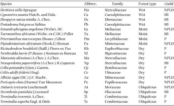
Table 1. The 20 Ghanaian woody species studied, their family, ecological guild and preference for a different forest type based on Hall & Swaine (Reference HALL and SWAINE1981), Hawthorne (Reference HAWTHORNE1995), Hawthorne & Jongkind (Reference HAWTHORNE and JONGKIND2006) and Hawthorne & Gyakari (Reference HAWTHORNE and GYAKARI2006). NPLD, Non-pioneer light demander; SB, Shade bearer; P, Pioneer.

Climate data
Nineteen climatic variables were obtained from the Worlclim database (Hijmans et al. Reference HIJMANS, CAMERON, PARRA, JOHNS and JARVIS2005). The data were derived from a compilation of monthly averages of climatic variables measured from a large number of weather stations across the globe, mostly between the periods 1950–2000 (Hijmans et al. Reference HIJMANS, CAMERON, PARRA, JOHNS and JARVIS2005). These data were interpolated using ANNUSPLIN to create a global climate dataset meaningful for ecological analysis. The dataset has a 1-km resolution and consists of 19 climatic variables. For details see Hijmans et al. (Reference HIJMANS, CAMERON, PARRA, JOHNS and JARVIS2005). We used plot coordinates and in some cases forest reserve coordinates to estimate the values of each of the 19 climatic variables for the study locations. We consider the Wordclim data to be of sufficient resolution for our study. Fauset et al. (Reference FAUSET, BAKER, LEWIS, FELDPAUSCH, AFFUM-BAFFOE, FOLI, HAMER and SWAINE2012) have shown that habitat scores on the ordination axis 1 of Hall & Swaine (Reference HALL and SWAINE1976, Reference HALL and SWAINE1981) and Hawthorne & Abu-Juam (Reference HAWTHORNE and ABU-JUAM1995) are strongly correlated with precipitation data from the Worldclim data. This same axis is also correlated with rainfall data (data from 5 y prior to 1963) from 170 weather stations in Ghana used in the classification of forest types by Hall & Swaine (Reference HALL and SWAINE1976). In the Worldclim database variation in the density of climatic stations was taken into account in the generation of the bioclimatic variables (details in Hijmans et al. Reference HIJMANS, CAMERON, PARRA, JOHNS and JARVIS2005). Our plots were located inside forest reserves and their microclimate is relatively less disturbed, although past disturbance may have led to increased dryness of the forest and to an increase in the presence of light-demanding species.
Selection of climatic variables
A principal component analysis (PCA) (Appendix 2) was conducted to evaluate how all 19 climatic variables were associated for the 2505 plots. The first two PCA axes explained 81% of the variation. We selected four climatic variables that described the two main axes of climatic variation and that were relatively independent from each other; annual rainfall and rainfall seasonality (the coefficient of variation of mean monthly rainfall, in %), temperature seasonality (calculated as standard deviation of mean monthly temperature × 100, in °C), and isothermality (the ratio of mean diurnal temperature range and annual temperature range × 100, in %). An isothermality value of 100 represents a site where the diurnal temperature range is equivalent to the annual temperature range. Values less than 100 indicate a smaller level of diurnal temperature variability (mean of monthly (maximum–minimum temperature)) relative to the temperature variability in a year (maximum temperature of the warmest month–minimum temperature of the coldest month). The selection of the four variables was also based on the fact that they reflected a resource (rainfall) and an important condition (temperature) that physiologically affects the growth of plants (Pausas & Austin Reference PAUSAS and AUSTIN2001), and are predicted to change with climate change. Seasonality may represent a bottleneck for plant performance (Clark et al. Reference CLARK, CLARK and OBERBAUER2010). Isothermality has been shown to influence plant height growth across latitudes though the relationship is weak (Moles et al. Reference MOLES, WARTON, WARMAN, SWENSON, LAFFAN, ZANNE, PITMAN, HEMMINGS and LEISHMAN2009). Temperature seasonality is important for species growth and hence for their distribution because most annual net primary production of trees in seasonal forests is concentrated in the months with high rainfall and growth is likely to be most sensitive to temperature variability during this time of the year (Vlam et al. Reference VLAM, BAKER, BUNYAVEJCHEWIN and ZUIDEMA2014). All four variables were moderately to highly correlated with one of the first two PCA axes. The first axis of the PCA explained 46% of the variation and showed a strong Pearson correlation with annual rainfall (r = 0.93), temperature seasonality (r = 0.66) and isothermality (r = 0.73). Rainfall seasonality also was moderately correlated with the second axis (r = 0.50) that explained 35% of the variation. We tested for multicollinearity among the four variables using collinearity statistics. The variance inflation factor was < 3 indicating that all four variables could be included in a regression analysis (Zuur et al. Reference ZUUR, IENO and ELPHICK2010). Correlations among the four variables are shown in Appendix 3.
Species response to climatic variables
For each of the species, we conducted a forward multiple logistic regression analysis of presence/absence on the four climatic variables and their quadratic terms. To be able to construct bell-shaped responses both the simple and quadratic terms for each climatic variable were included. We also included interaction terms but the interactions contributed little to the variation (data not shown). For each species the regression model with the lowest deviance (−2 log likelihood) and highest Nagelkerke R2 was selected (Field Reference FIELD2009). Area under the curve (AUC) of a receiver operating characteristic curve (ROC) (Metz Reference METZ1978) was used to measure the overall model accuracy (Pearce & Ferrier Reference PEARCE and FERRIER2000). We interpreted AUC using the scale proposed by Swets (Reference SWETS1988): good = AUC > 0.9; useful = 0.9 > AUC > 0.7 and poor AUC < 0.7. The partial variation contributed by each environmental variable was calculated as the increase in variation when the variable was included in the model. Parameters (Appendix 4) derived from the species-specific regression models were used to calculate the probability of occurrence for each species for all four environmental variables using the formula: P = 1/ (1 + Exp (−bo−b1×1−b2×12 . . . . . . . . . . .−b7×4−b8×42)), where P = probability of occurrence, Exp = exponential, bo = a constant, X1–4 = the four bioclimatic variables used, b1–b8 = coefficients for the four bioclimatic variables and their quadratic terms.
We constructed the response curves for each species against the individual climatic variables using the calculated probabilities, while keeping the other three climatic factors constant. When we kept the other three environmental variables constant, we used their mean values across all 2505 plots in Ghana. Using constant values for the other variables is the only way to directly compare the response curves of different species to an individual climatic variable. We acknowledge that individual species may have their peak occurrence in different parts of the climate space for the other three climatic variables than the mean values for Ghana that we used, which may lead to over- or underestimations of the responses at some part of the climatic gradient for a particular species. The mean values used were 1514 mm y−1 for annual rainfall, 53% (coefficient of variation) for rainfall seasonality, 72% for isothermality and 1028°C for temperature seasonality (temperature seasonality being calculated as standard deviation of mean monthly temperature ×100). The temperature data were in units of °C ×10. Hence this means that in normal degrees the average temperature seasonality for the plots is 1.028°C. Species rainfall optimum (Ropt) and range (Rrange) were derived from the species response curves. Rainfall optimum was the value at which species occurrence reached the maximum (ecological optimum). Rrange was the range of rainfall conditions under which the species occur computed as the difference between the minimum rainfall (rainfall at the 10th percentile) and the maximum rainfall (rainfall at the 90th percentile) (Maharjan et al. Reference MAHARJAN, POORTER, HOLMGREN, BONGERS, WIERINGA and HAWTHORNE2011). All statistical analyses were conducted using Predictive Analytics Software (PASW) statistics for windows version 18.0 (SPSS Incorporated, Chicago, IL).
RESULTS
Relative importance of climatic variables for species distribution
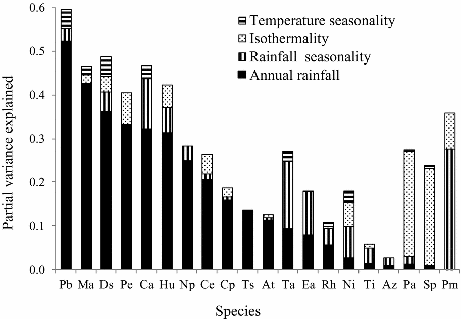
Species showed different responses to the four climatic variables studied. Most of the selected regression models (75%) had AUC > 0.7 (Appendix 4) indicating that the models are useful for predicting the occurrence of species using the four climatic variables and presence-absence data. Most of the 20 woody species (95%) showed a significant response to rainfall, followed by rainfall seasonality (60%), isothermality (45%) and temperature seasonality (40%). The logistic regression models explained on average 28% (range = 3–60% across species) of the variation in species occurrence. On average, 17% (range = 0.8–52%) of the variation in species occurrence was explained by annual rainfall, 5% (range = 0.5–27.5%) by rainfall seasonality, 4% (range = 0.8–24%) by isothermality and 1% (range = 0.4–4.5%) by temperature seasonality. For 12 of the 20 species annual rainfall explained, amongst the four factors studied, most of the variation in occurrence (Figure 1). Examples of species affected by annual rainfall are: Heritiera utilis and Pentadesma butyracea, which are typical wet-forest species; Mansonia altissima, which is a typical dry-forest species; and Terminalia superba, which is found in all main (wet, moist and dry) forest types in Ghana (Figures 1 and 2). For six of the species rainfall seasonality explained most of the variation of the four factors studied and these were mostly species with peak occurrence in moist forests such as Entandrophragma angolense and Turraeanthus africanus (Figures 1 and 2). For two of the species (Strombosia pustulata and Piptadeniastrum africanum), isothermality explained most of the variation in occurrence with reference to the four factors studied. Temperature seasonality did not explain the most (of four factors studied) important variation in the occurrence for any of the 20 species studied (Figure 1).
Figure 1. Bar graph displaying variation in species occurrence explained by four climatic variables in multiple logistic regression models for 20 Ghanaian woody tree species. Climatic variables included are: RAN, annual rainfall; RSEAS, rainfall seasonality; ISO, isothermality; TSEAS, temperature seasonality. The species are ordered based on the variation explained by annual rainfall. At, Antiaris toxicaria; Az, Albizia zygia; Ca, Cynometra ananta; Ce, Celtis adolfi-friderici; Cp, Ceiba pentandra; Ds, Diospyros sanza-minika; Ea, Entandrophragma angolense; Hu, Heritiera utilis; Ma, Mansonia altissima; Ni, Newbouldia laevis; Np, Nesogordonia papaverifera; Pa, Piptadeniastrum africanum; Pb, Pentadesma butyracea; Pe, Pericopsis elata; Pm, Petersianthus macrocarpus; Rh, Ricinodendron heudelotii; Sp, Strombosia pustulata; Ta, Turraeanthus africanus; Ti, Terminalia ivorensis; Ts, Terminalia superba.
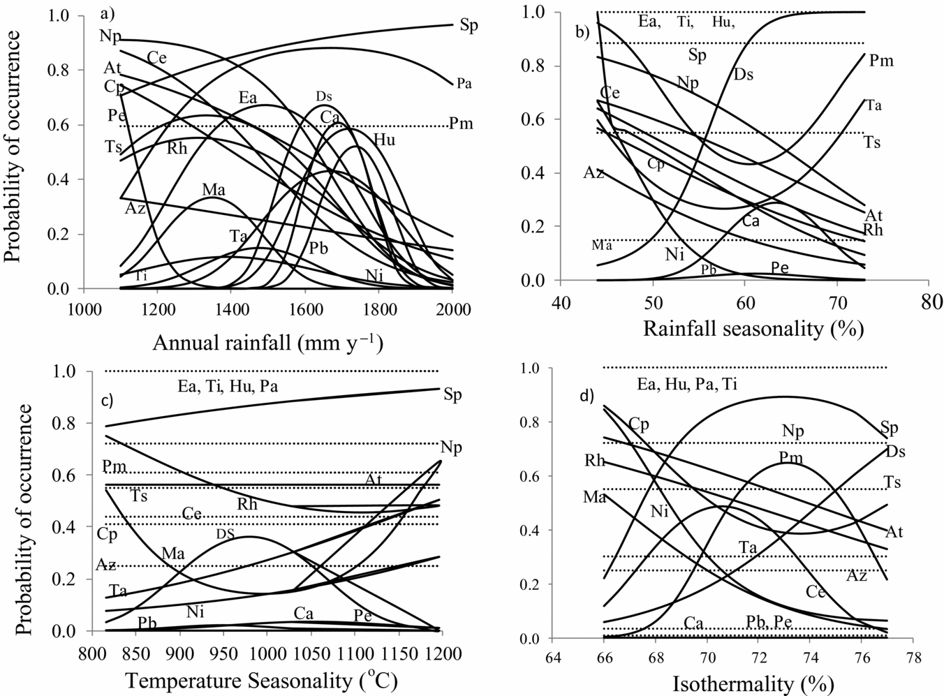
Figure 2. Species response curves showing the probability of occurrence of 20 tropical woody tree species of Ghana in relation to annual rainfall, rainfall seasonality, isothermality and temperature seasonality. Curves give the results of fitted logistic regression models (Appendix 4). The temperature data were in units of °C ×10. Hence temperature seasonality values have been multiplied by 1000. At, Antiaris toxicaria; Az, Albizia zygia; Ca, Cynometra ananta; Ce, Celtis adolfi-friderici; Cp, Ceiba pentandra; Ds, Diospyros sanza-minika; Ea, Entandrophragma angolense; Hu, Heritiera utilis; Ma, Mansonia altissima; Ni, Newbouldia laevis; Np, Nesogordonia papaverifera; Pa, Piptadeniastrum africanum; Pb, Pentadesma butyracea; Pe, Pericopsis elata; Pm, Petersianthus macrocarpus; Rh, Ricinodendron heudelotii; Sp, Strombosia pustulata; Ta, Turraeanthus africanus; Ti, Terminalia ivorensis; Ts, Terminalia superba. Annual rainfall (a), rainfall seasonality (coefficient of variation) (b), temperature seasonality (calculated as standard deviation of mean monthly temperature × 100) (c), and isothermality (ratio of mean diurnal temperature range and annual temperature range × 100) (d).
Species response to climatic variables
Species showed different response curve types to the four climatic variables studied: unimodal response (Figure 3a), decreasing response (Figure 3b), increasing response (Figure 3c), and flat response, indicating no response. On average 31% (25 of 80) of the response curves were unimodal and such responses were mostly found with respect to the rainfall gradient (12 out of 20 species) and least with respect to isothermality (4 of 20 species). Decreasing response was mostly found with respect to rainfall seasonality (7 of 20 species) and least with respect to isothermality (4 of 20 species). Increasing response was mostly associated with temperature seasonality (3 of 20) and least with rainfall (1 of 20 species). Flat response was mostly associated with temperature seasonality (12 of 20 species) and isothermality (11 of 20 species) (Table 2). Examples of species that showed different response curves are Diospyros sanza-minika, which showed a unimodal response to annual rainfall (Figure 2a) but an increasing response to rainfall seasonality and isothermality (Figure 2b, d). Strombosia pustulata (Sp) showed an increasing response curve to annual rainfall (Figure 2a) but unimodal response to isothermality (Figure 2d).
Table 2. Number of Ghanaian forest tree species (n = 20) that show different types of response curves, in response to four climatic factors.
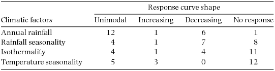
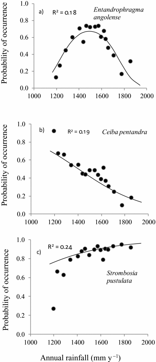
Figure 3. Examples of different species response curves of three of 20 Ghanaian woody tree species to annual rainfall. Species responses (in terms of probability of occurrence) are fitted with logistic regression models. Regression lines show the predicted occurrence in relation to rainfall, while the three other climatic factors (rainfall seasonality, temperature seasonality and isothermality) are kept constant. Dots show the average observed probability of occurrence for rainfall class intervals of 150 plots. To make sure that each rainfall class contained 150 plots, the rainfall classes had variable widths. Unimodal response (a), decreasing response (b) and increasing response (c).
DISCUSSION
We analysed the environmental response curves of 20 important Ghanaian timber species and determined the relative importance of rainfall and temperature to their distribution. Species showed differential responses to the climatic variables but the distributions of most species were more strongly influenced by rainfall than by temperature.
Importance of annual rainfall, temperature and their seasonality for species distribution
Rainfall
This study focused on the relative importance of annual rainfall and its seasonality, temperature seasonality and isothermality for species occurrence and tested the hypothesis that most of the species will respond to annual rainfall and especially rainfall seasonality. We found that nearly all (95%) species were significantly affected by annual rainfall and that annual rainfall explained more (on average 17%) of the variation in species occurrence than the other three factors evaluated (Figure 2). Other studies also found that rainfall was the main driver of large-scale distribution patterns of tropical plant and tree species (Bongers et al. Reference BONGERS, POORTER, VAN ROMPAEY and PARREN1999, Holmgren & Poorter Reference HOLMGREN and POORTER2007, Maharjan et al. Reference MAHARJAN, POORTER, HOLMGREN, BONGERS, WIERINGA and HAWTHORNE2011, Toledo et al. Reference TOLEDO, POORTER, PEÑA-CLAROS, ALARCÓN, BALCÁZAR, CHUVIÑA, LEAÑO, LICONA, TER STEEGE and BONGERS2011, Reference TOLEDO, PEÑA-CLAROS, BONGERS, ALARCÓN, BALCÁZAR, CHUVIÑA, LEAÑO, LICONA and POORTER2012). It is surprising that rainfall seasonality explained only 5% of the variation contrary to the widely held view that it strongly influences species distribution (Borchert Reference BORCHERT1998, Kato et al. Reference KATO, ITIOKA, SAKAI, MOMOSE, YAMANE, HAMID and INOUE2000). In a recent study, dry-season intensity was found to be among the main drivers of individual species distribution in Panama (Condit et al. Reference CONDIT, ENGELBRECHT, PINO, PÉREZ and TURNER2013). The, at first sight, low percentage variation explained by annual rainfall may have resulted from the small plot size (1-ha) used. The smaller plot size, however, allowed more replicates, and thus a higher statistical power to detect independent variation of various climatic variables affecting the distribution of the species.
Recently, Fauset et al. (Reference FAUSET, BAKER, LEWIS, FELDPAUSCH, AFFUM-BAFFOE, FOLI, HAMER and SWAINE2012) evaluated the effects of drought on changes in plants’ functional composition and biomass over a 20-year period in a variety of forest types in Ghana. They found that during this period wet-forest evergreen and subcanopy shade-tolerant species decreased in abundance, whereas dry-forest deciduous and canopy species increased in abundance. It is possible that these changes are not only driven by an increase in drought, but also by general increasing levels of disturbance in the forest zone of Ghana over the sampled period. Drier climate coupled with other human activities may result in incidence of fire which leads to further changes in forest composition. Experimental studies (field: Engelbrecht et al. Reference ENGELBRECHT, COMITA, CONDIT, KURSAR, TYREE, TURNER and HUBBELL2007, Nepstad et al. Reference NEPSTAD, TOHVER, RAY, MOUTINHO and CARDINOT2007; greenhouse: Deines et al. Reference DEINES, HELLMANN and CURRAN2011) showed that seasonal drought has a strong effect on growth and survival of individual tree species, and that drought tolerance is a good predictor of species distribution along the rainfall gradient (Baltzer et al. Reference BALTZER, DAVIES, BUNYAVEJCHEWIN and NOOR2008, Engelbrecht et al. Reference ENGELBRECHT, COMITA, CONDIT, KURSAR, TYREE, TURNER and HUBBELL2007, Sterck et al. Reference STERCK, MARKESTEIJN, TOLEDO, SCHIEVING and POORTER2014). Repeated incidental (El Niño) drought also resulted in high mortality of especially trees with low wood density in the Amazon forest (Phillips et al. Reference PHILLIPS, VAN DER HEIJDEN, LEWIS, LOPEZ-GONZALEZ, ARAGAO, LLOYD, MALHI, MONTEAGUDO, ALMEIDA, DAVILA, AMARAL, ANDELMAN, ANDRADE, ARROYO, AYMARD, BAKER, BLANC, BONAL, DE OLIVEIRA, CHAO, CARDOZO, DA COSTA, FELDPAUSCH, FISHER, FYLLAS, FREITAS, GALBRAITH, GLOOR, HIGUCHI, HONORIO, JIMENEZ, KEELING, KILLEEN, LOVETT, MEIR, MENDOZA, MOREL, VARGAS, PATINO, PEH, CRUZ, PRIETO, QUESADA, RAMIREZ, RAMIREZ, RUDAS, SALAMAO, SCHWARZ, SILVA, SILVEIRA, SLIK, SONKE, THOMAS, STROPP, TAPLIN, VASQUEZ and VILANOVA2010). Additionally, in an Amazonian forest an experimental drought caused a rapid and strong decline in above-ground wood production (Brando et al. Reference BRANDO, NEPSTAD, DAVIDSON, TRUMBORE, RAY and CAMARGO2008). In combination, these studies suggest that species drought tolerance is a major determinant explaining species distribution along the rainfall gradient. However, other associated factors such as soil fertility, herbivory and pathogens, and perhaps most significantly, natural and human-induced disturbances such as forest fire, large wind blows and selective logging, can also co-influence species distribution along the rainfall gradient. Disturbance (and density of light-demanding species) also increases with dryness of forest type (Hawthorne Reference HAWTHORNE1996). In addition, dispersal limitation may also influence the distribution of species (Duncan et al. Reference DUNCAN, CASSEY and BLACKBURN2009). In general, soil fertility declines with increasing rainfall in Ghana and Panama (Brenes-Arguedas et al. Reference BRENES-ARGUEDAS, RÍOS, RIVAS-TORRES, BLUNDO, COLEY and KURSAR2008, Swaine Reference SWAINE1996, Veenendaal & Swaine Reference VEENENDAAL, SWAINE, Newbery, Prins and Brown1998), probably because soils in wetter areas are more leached as has been shown for Ghana (Swaine Reference SWAINE1996). Controlled experiments that evaluated species growth responses to different wet-, moist- and dry-forest soils in Ghana (L. Amissah et al. unpubl. data, Veenendaal et al. Reference VEENENDAAL, SWAINE, LECHA, WALSH, ABERBRESE and OWUSU-AFRIYIE1996) found that the growth of very few species was significantly affected by these soil differences. Planted seedlings in Panama showed a higher overall growth in soils from the drier part of the Isthmus than in soils from the wetter part. Insect herbivore damage and pathogen mortality were more associated with wet forest than dry forest in Panama, suggesting an increasing pest pressure along the rainfall gradient (Brenes-Arguedas et al. Reference BRENES-ARGUEDAS, COLEY and KURSAR2009). However, no significant differences in pest attack levels of wet-forest species and dry-forest species were found. Brenes-Arguedas et al. (Reference BRENES-ARGUEDAS, COLEY and KURSAR2009) concluded therefore, that seasonal drought was a stronger determinant of species distribution than pests.
Although the projection of future climate for West Africa is not unequivocal (Christensen et al. Reference CHRISTENSEN, HEWITSON, BUSUIOC, CHEN, GAO, HELD, JONES, KOLLI, KWON, LAPRISE, MAGAÑA RUEDA, MEARNS, MENÉNDEZ, RÄISÄNEN, RINKE, SARR, WHETTON, Soloman, Qin, Manning, Chen, Marquis, Averyt, Tignor and Miller2007), Sheffield & Wood (Reference SHEFFIELD and WOOD2008) found several IPCC models (IPCC-Assessment Report 4) predicting a reduction in precipitation and increased frequency in long-term soil drought for some subtropical and tropical regions, including West Africa. Furthermore, the precipitation trend in West Africa shows reduction in rainfall (Malhi & Wright Reference MALHI and WRIGHT2004) and increasing seasonality (Borchert Reference BORCHERT1998). Annual rainfall over the past two decades in some forest types in Ghana shows a 22.8% reduction in dry-season rainfall compared with pre-1970 levels (Fauset et al. Reference FAUSET, BAKER, LEWIS, FELDPAUSCH, AFFUM-BAFFOE, FOLI, HAMER and SWAINE2012). Additionally, rainfall is predicted to be reduced by 20% in 2050 in Ghana (Government of Ghana 2011). Most forest species are likely to shift their distribution in response to these trends and predictions. In particular for Ghana the distribution of species such as Heritiera utilis and Pentadesma butyracea that are sensitive to experimental drought (L. Amissah unpubl. data) may shift towards currently wetter forest areas in the south-west of the country.
Temperature
Isothermality co-explained the distribution of only 10% of the species. Mansonia altissima and Newbouldia laevis, for instance, showed steep decline in response to an increase in isothermality suggesting that the probability of occurrence of the species may be reduced with larger temperature variability within an average month relative to the year. This seems to contrast sharply with the results from a study in lowland Bolivia, where 72% of the 100 studied species showed a significant response to temperature (Toledo et al. Reference TOLEDO, PEÑA-CLAROS, BONGERS, ALARCÓN, BALCÁZAR, CHUVIÑA, LEAÑO, LICONA and POORTER2012). Temperature may have an indirect effect on plant growth. Short-term leaf-level measurements in a number of tropical forest regions showed that net carbon assimilation declines with an increase in daytime temperatures (Doughty & Goulden Reference DOUGHTY and GOULDEN2008). Similarly, eddy-flux towers in Brazil and Costa Rica showed a reduced net carbon uptake in the warmest daytime period (Doughty & Goulden Reference DOUGHTY and GOULDEN2008, Goulden et al. Reference GOULDEN, MILLER, DA ROCHA, MENTON, DE FREITAS, E SILVA FIGUEIRA and DE SOUSA2004, Loescher et al. Reference LOESCHER, OBERBAUER, GHOLZ and CLARK2003). Field studies in tropical forests in Costa Rica, Malaysia and Panama also showed negative correlation between tree growth and temperature (Clark et al. Reference CLARK, PIPER, KEELING and CLARK2003, Feeley et al. Reference FEELEY, WRIGHT, NUR SUPARDI, KASSIM and DAVIES2007). In many countries (like Ghana) where seasonal variability in temperature is large compared to daily variation, predicted increases in temperature may affect the distribution of limited number of species. However, in areas with larger temperature variation, such as the southern edge of the Amazon where cold winds from Patagonia penetrate for short spells, increases in temperature are likely to shift the distribution of more species (Toledo et al. Reference TOLEDO, PEÑA-CLAROS, BONGERS, ALARCÓN, BALCÁZAR, CHUVIÑA, LEAÑO, LICONA and POORTER2012).
Shapes of species response curves to environmental gradients
We hypothesized that unimodal response curves will more often be found in relation to the annual rainfall gradient than to the temperature gradient, because under relatively benign conditions environmental resources (such as water) are more important in shaping species responses than environmental conditions such as temperature. Most species (60%) indeed showed a unimodal response to rainfall, whereas 30% of the species showed decreased and 5% increased occurrence with rainfall across Ghana. In contrast, only 20–25% of the species exhibited a unimodal response curve to isothermality and temperature seasonality. This could have been attributed to effects of shorter gradient length for temperature, but in our study this was not the case: in fact the gradients were similarly long with 1.5-fold variation for temperature and 1.7-fold variation for rainfall (Appendix 1). Other studies on tropical tree species found a similar or lower number of unimodal response curves; 56% of the studied species along a rainfall gradient in West Africa (Maharjan et al. Reference MAHARJAN, POORTER, HOLMGREN, BONGERS, WIERINGA and HAWTHORNE2011), 42% of the species along a soil-fertility gradient in North-West Amazonia (Duque Reference DUQUE2004), and 25% and 10% along a rainfall and temperature gradient respectively in Bolivia (Toledo et al. Reference TOLEDO, PEÑA-CLAROS, BONGERS, ALARCÓN, BALCÁZAR, CHUVIÑA, LEAÑO, LICONA and POORTER2012). We acknowledge that these results are not directly comparable as they are also dependent on the species number and selection criteria and on the length and the type of the gradient used.
The shape of a species response curve is determined by the length of the gradient and species-specific properties such as tolerance and the position of the optimum (Austin & Smith Reference AUSTIN and SMITH1989, Rydgren et al. Reference RYDGREN, ØKLAND and ØKLAND2003). Generally if the gradient is long, unimodal curves are expected (Gauch & Whittaker Reference GAUCH and WHITTAKER1972, Oksanen & Minchin Reference OKSANEN and MINCHIN2002), but if the optimum of the species is close or beyond the extreme end of the gradient truncated curves are expected (Rydgren et al. Reference RYDGREN, ØKLAND and ØKLAND2003, ter Braak & Looman Reference TER BRAAK and LOOMAN1986). Few unimodal response curves were found for temperature seasonality and isothermality and 55–60% of the species showed no response. Other environmental factors may drive the shape of the response curve for these species (Austin & Gaywood Reference AUSTIN and GAYWOOD1994, Duque Reference DUQUE2004), overruling temperature seasonality and isothermality. In sum, this study shows that annual rainfall and seasonality are the main climatic factors influencing distribution of individual tree species in Ghana, though temperature influences the distribution of some species. Predicted increases in frequency and severity of drought may cause shifts in the distribution of species that occur at the wetter side of the rainfall gradient.
ACKNOWLEDGEMENTS
LA was supported by a grant from Wageningen University and the Netherlands Fellowship Programme (NUFFIC). We thank Dr Mike Swaine for providing advice on species selection and allowing us to use his database of species and their ordination scores, and an anonymous reviewer for their helpful comments.
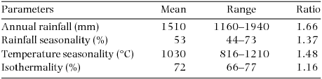
Appendix 1. Mean, range and ratio (maximum divided by the minimum) of climatic variables of 2505 forest plots of Ghana. The mean, range and ratio are based on climatic data obtained from the Worldclim database (Hijmans et al. Reference HIJMANS, CAMERON, PARRA, JOHNS and JARVIS2005).
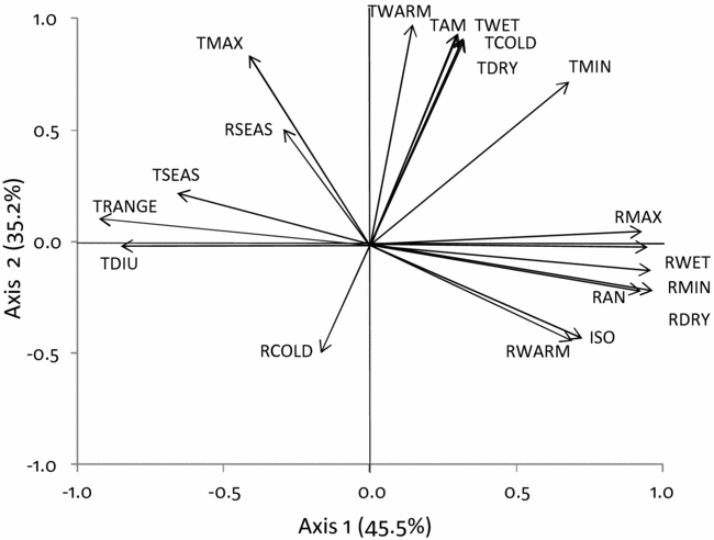
Appendix 2. Principal Components Analysis (PCA) on 19 climatic variables for 2505 forest sites in Ghana. The first and second axes explain respectively 46% and 35% of the variation. RAN, annual precipitation; TSEAS, temperature seasonality; RSEAS, precipitation seasonality; ISO, isothermality; TAM, annual mean temperature; TDIU, temperature mean diurnal range; TMAX, max temperature of warmest month; TMIN, min temperature of coldest month; TRANGE, temperature annual range; TWET, mean temperature of wettest quarter; TDRY, mean temperature of driest quarter; TWARM, mean temperature of warmest quarter; TCOLD, mean temperature of coldest quarter; RMAX, precipitation of wettest month; RMIN, precipitation of driest month; RWET, precipitation of wettest quarter; RDRY, precipitation of driest quarter; RWARM, precipitation of warmest quarter; RCOLD, precipitation of coldest quarter. The climatic variables were obtained from the Worldclim database (Hijmans et al. Reference HIJMANS, CAMERON, PARRA, JOHNS and JARVIS2005).
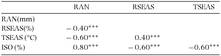
Appendix 3. Pearson correlations among annual rainfall (RAN), rainfall seasonality (RSEAS), temperature seasonality (TSEAS) and isothermally (ISO) and their P values. ***P ≤ 0.001, n = 2505. The four climatic variables are for 2505 1-ha forest plots in Ghana. The climatic variables were obtained from the Worldclim database (Hijmans et al. Reference HIJMANS, CAMERON, PARRA, JOHNS and JARVIS2005).

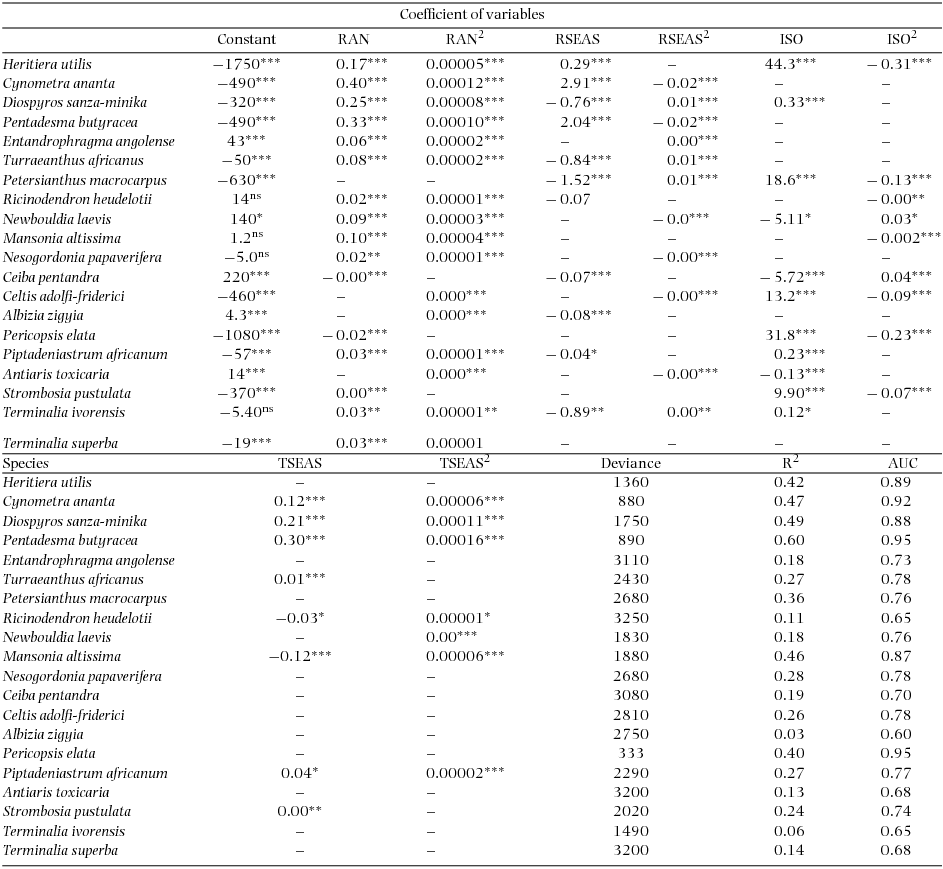
Appendix 4. Regression models fitted for presence absence data of 20 woody tree species of Ghana, the deviance (−2 log likelihood), Nagelkerke R2, significant levels, and model accuracy; Area Under the Curve (AUC). RAN, annual rainfall; RSEAS, rainfall seasonality; ISO, isothermality; TSEAS, Temperature seasonality. Significant levels are at *P < 0.05, **P < 0.01, ***P < 0.001, ns = not significant.