


I. Introduction
With retail sales of $212,172M, the U.S. alcoholic beverage market is slightly smaller than China ($249,716M), the largest market, and substantially larger than Japan ($88,676M), the third largest market.Footnote 1 The production of alcoholic beverages within the United States is also substantial, and the Distilled Spirits Council of the United States estimated that the total direct economic value of the domestic alcoholic beverage sector in 2015 was $212.2B.Footnote 2
Although alcohol is an important consumption good and domestic alcohol production an important industry, excessive alcohol consumption is associated with substantial negative health outcomes and large externality costs (Sacks et al., Reference Sacks, Roeber, Bouchery and Gonzales2013; Sacks et al., Reference Sacks, Gonzales, Bouchery and Tomedi2015). In addition to the evidence on the negative effects of excessive alcohol consumption (see Holmes et al. (Reference Holmes, Meier, Booth and Guo2012) for a review), there is also evidence that externality costs vary with beverage type. For example, Naimi et al. (Reference Naimi, Brewer, Miller and Okoro2007) find beer to be over-represented in binge drinking incidents in the United States; and beer consumption is over-represented, relative to its consumption share, in drunk driving incidents (Kerr and Ye, Reference Kerr and Ye2011; Berger and Snortum, Reference Berger and Snortum1985; Colón and Cutter, Reference Colón and Cutter1983). The U.S. evidence on liver cirrhosis mortality also suggests the strongest association is with spirits rather than beer or wine (Ye and Kerr, Reference Ye and Kerr2011; Ponicki and Gruenewald, Reference Ponicki and Gruenewald2006; Cohen, Mason, and Farley, Reference Cohen, Mason and Farley2004; Gruenewald and Ponicki, Reference Gruenewald and Ponicki1995; Roizen, Kerr, and Fillmore, Reference Roizen, Kerr and Fillmore1999). Spirits are also found to be the dominant beverage for binge drinking involving U.S. youth (Naimi et al., Reference Naimi, Siegel, DeJong and O'Doherty2015; Siegel et al., Reference Siegel, Naimi, Cremeens and Nelson2011).
It is valuable to understand the trends and possible future patterns for alcohol consumption by beverage type given that the consumption of some alcoholic beverage types tends to be more strongly correlated with outcomes or actions that increase externality costs and negative health outcomes. Alcohol consumption forecasts can also be compared to policy settings to gain insights on the relative effectiveness of different alcohol use control policies, including alcohol taxes.
In this research United States’ state level per capita alcohol consumption data are used to investigate trends in consumption patterns and forecast future consumption trends, and investigate the extent of convergence in alcohol consumption patterns across states. The alcohol policy environment in each state is then compared to consumption forecast information to try and identify the impact of policy settings on forecast consumption trends.
II. Data and Methods
A. Data
Alcohol consumption data are derived from LaVallee, Kim, and Yi (Reference LaVallee, Kim and Yi2014), and represent average per capita (14+) ethanol consumption from beer, wine, and spirits, where the conversion rates to ethanol are based on average alcohol by volume rates of 4.8% for beer, 12.5% for wine, and 40% for spirits. The source data covers the period between 1972 to 2012. State level tax rate information is based on the Tax Foundation values, converted to pure alcohol tax rate equivalents. Federal tax rate information is based on excise tax information. Policy setting information is based on the ratings in the various Centers for Disease Control and Prevention policy report cards. The report cards use a red, yellow, and green evaluation system, and provide information on taxation, the extent of commercial host liability laws, and the ability to regulate outlet density.Footnote 3
B. Visual Data Display
The analysis considers beer, wine, and spirit consumption, and the data are displayed via a series of ternary plots. In each plot the overall level of consumption is illustrated via the size of the dot. The way the consumption share data on state level per capita beer, wine, and spirit consumption are mapped to each ternary plot is shown in Figure 1. The specific software used to generate the ternary plots was Hamilton (Reference Hamilton2016).
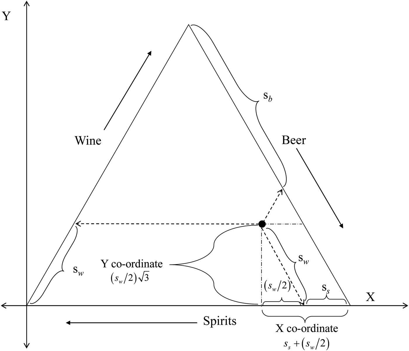
Figure 1 The Geometry of Alcohol Consumption
C. Convergence Measures
The first measure used to track convergence was the change in the coefficient of variation for per capita consumption for each beverage, where the coefficient of variation was defined as  $\sigma_{it}/\bar {\rm X}_{it},$ where σ it denoted the standard deviation of per capita consumption for beverage i at time t, and
  $\bar {\rm X}_{it}$ denoted the average level of per capita consumption for beverage i at time t.
In addition to an individual beverage measure, we follow the approach of Holmes and Anderson (Reference Holmes and Anderson2017) and use the similarity index presented in Anderson (Reference Anderson2014) to calculate a similarity index value, for each state that includes information on the differences between individual state level ethanol consumption shares and the average ethanol consumption share for all three beverages. The specific measure we calculate can be defined as follows. Let s ijt denote the ethanol share for beverage i, in state j, at time t; and let  $\bar s_{it}$ denote the average ethanol share for beverage i at time t across all states. The overall similarity index value for state j, at time t, can then be found as:
  $W_{jt} = \sum {_i s} _{ijt}.\bar s_{it}/(\sum {_i s} _{ijt}^2 )^{1/2}.(\sum {_i \bar s} _{it}^2 )^{1/2}$, where the metric converges to one for equality between the consumption pattern in state j and the average, and tends to zero the more dissimilar the consumption mix in state j is to the average. We then calculate the mean, standard deviation, and coefficient of variation for the index.
One criticism of the similarity index measure used in Holmes and Anderson (Reference Holmes and Anderson2017), when applied to ethanol or budget share information, was that the adding-up constraint places restrictions on the covariance relationships across beer, wine, and spirits. The specific restrictions on the covariances are set out in detail in Mills (Reference Mills2018), and in light of these issues Mills (Reference Mills2018) suggested using the trace of a matrix that was calculated as the centred log-ratio of covariances. The specific convergence measure is tr(Γt), where,  $\Gamma _t = [{\mathop{\rm cov}} \{ \log ({\bi s}_{it}/{\bi S}_t),\;\log ({\bi s}_{kt}/{\bi S}_t)\} $ : i, k = beer, wine, spirits, where sit = s i1t, s i2t, …s iJt, and
  $S_t = [(s_{b1t}.s_{w1t}.s_{s1t})^{{\textstyle{1 \over 3}}}(s_{b2t}.s_{w2t}.s_{s2t})^{{\textstyle{1 \over 3}}}...\;(s_{bJt}.s_{wJt}.s_{sJt})^{{\textstyle{1 \over 3}}}]^T,$ and this measure flows from the work of Aitchison (Reference Aitchison1982, Reference Aitchison2003).
D. Forecasts
The beverage specific consumption forecasts have been developed using the ARIMA methodology. With B denoting the backshift operator such that By t = y t−1, it is conventional to write the general form of an ARIMA model for the series y t as (1 − φ 1 − B − … − φ pB p)y t = c + (1 + θ 1B + … + θ qB q)e t. However, it terms of understanding the steps involved in developing the forecasts it can be easier to think of using a two-step process. The first step is to determine the order of integration, and the second step is to determine the appropriate number of moving average (MA) and autoregressive (AR) parameters to use in the forecast model.
Methods to test for stationarity can be classified in terms of tests where the null hypothesis is that the data series is stationary, and tests where the null hypothesis is that the data series has a unit root. Here, to prevent over differencing, the KPSS test introduced in Kwiatkowski et al. (Reference Kwiatkowski, Phillips, Schmidt and Shin1992) is used to determine the order of integration. The null hypothesis for the KPSS test is that the data series is stationary. The alternative hypothesis is that the series has a unit root.
For each data series, following differencing (if required) an automated iterative process was used to search for the appropriate number of AR and MA terms. In the search process five MA terms and five AR terms were set as a predefined limit for the maximum number of terms in the model. For all models that are stationary, in levels or first differences, the possibility of including a constant term was also considered. For stationary in levels models the constant is interpreted as a non-zero mean term. In first difference stationary models the constant is interpreted as a drift term. For models differenced at least twice, a constant term is not considered. To select between different models BIC was used. Hyndman (Reference Hyndman2017) was used for estimation, and complete details on the estimation routines are explained in Hyndman and Khandakar (Reference Hyndman and Khandakar2008). Model selection and model fit details are reported in the Appendix.
E. Pair-Wise Comparisons of Consumption Changes
All pair-wise comparisons of consumption changes rely on Bayesian estimation methods. The case for using Bayesian estimation methods rather than t-tests is set out in Kruschke (Reference Kruschke2013), where it is shown that even for simple comparisons Bayesian methods have substantial advantages over traditional null hypothesis significance testing. As we follow Kruschke (Reference Kruschke2013), when reporting the estimation results we focus on reporting 95% Highest Density Intervals (HDI). Estimation relies on Kruschke and Meredith (Reference Kruschke and Meredith2017), and the default settings are used. This means that the data are modeled using a t-distribution with uninformative priors, and the MCMC chain length is 10,000, with no thinning, and the burn-in length is 1,000.
F. Policy Setting Comparisons
To investigate possible reasons for differences in forecast per capita consumption, for each beverage category, states were grouped into jurisdictions where consumption is forecast to increase, decrease, or remain constant. Comparisons across groups rely on the same methods described earlier.
III. Results
A. Total Per Capita Alcohol Consumption
To illustrate changes in total per capita consumption across the United States, Figure 2 plots state level average consumption levels at ten-year intervals, as well as forecast per capita consumption in 2022, which is ten years from the last year of source data. Figure 2 shows that over the period 1972 to 2002, both the total per capita alcohol consumption and the extent of dispersion in per capita consumption across states decreased; and that since 2002 there has been a slight increase in both the level of alcohol consumption and the level of dispersion. The state level alcohol consumption forecasts for 2022 suggest no further increases in average per capita consumption, but a continuing increase in dispersion across the states.
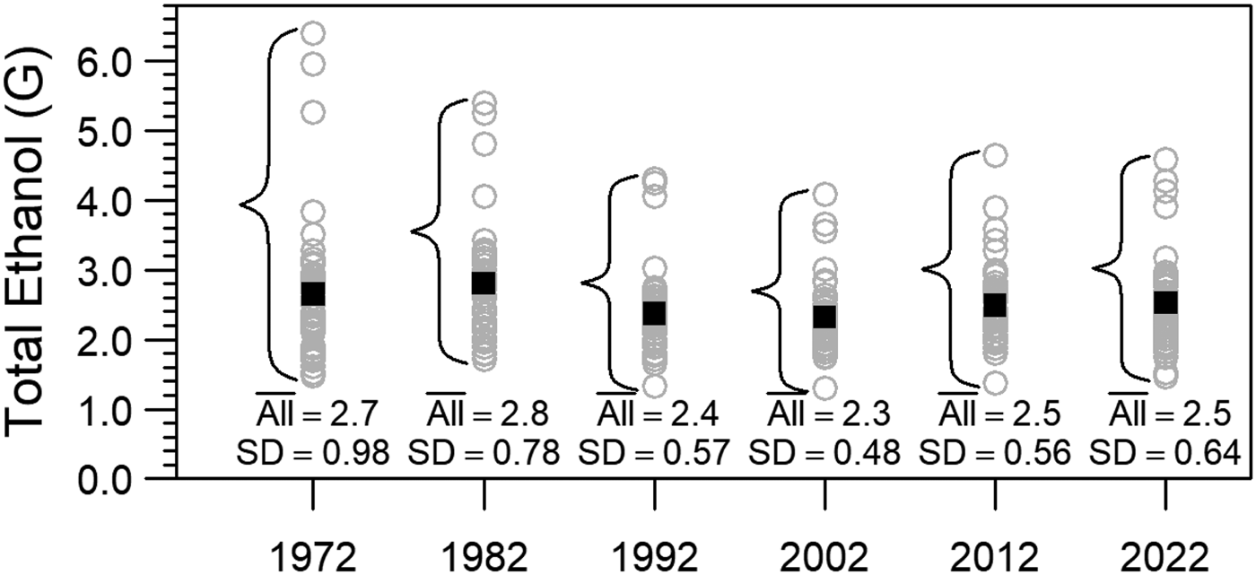
Figure 2 U.S. Per Capita Ethanol Consumption through Time
B. Beverage Specific Consumption Changes
In Figure 3 the position of each dot indicates the relative importance of each beverage in terms of the per capita consumption share, and the size of the dot reflects total per capita alcohol consumption. Similar to Figure 2, in Figure 3 both actual values and forecast values for 2022 are plotted. Considering Figure 3 as a whole reveals several key features of the U.S. alcoholic beverage market. First, over the period 1972 to 2012, the size of the largest dots tends to get smaller. This is evidence of a reduction in drinking in those states that have historically had the highest level of alcohol consumption. Second, between 1972 and 2002 the dots shift to the right, indicating an increase in the relative importance of beer at the expense of spirits. Third, between 2002 and 2012 there is an upward shift in the dots that indicates an increase in the relative importance of wine. Fourth, between 1972 and 1992 the dots became more clustered together, but then they start to move further apart again such that the variation in consumption preferences for beer, wine, and spirits across states in the forecast period looks about the same as that observed in 1972.

Figure 3 Beer, Wine, and Spirits Consumption in the United States
Table 1 provides information on the coefficient of variation through time for per capita consumption of each beverage, total per capita consumption, and the ethanol share similarity index. The trace of the log-ratio centered covariance matrix is also shown. These values can be seen as providing formal evidence on the changes in dispersion through time. For spirits, the measure indicates steady convergence from 1972 to 2012, and then an increase in dispersion for the forecast period; for wine we see convergence for the period 1972 to 1992 followed by an increase in dispersion; and for beer we see convergence over the period 1972 to 2002 followed by an increase in dispersion. For the total alcohol consumption measure we see a decrease in dispersion between 1972 and 2002, followed by an increase in dispersion. For the ethanol share index measure we see a decrease in dispersion between 1972 and 1992, followed by an increase in dispersion. One interpretation of the 2022 values for the total consumption measure and the index measure is that, relative to 1972, there will be less dispersion in the level of consumption in 2022, but slightly more variation in the consumption mix.
Table 1 Convergence Measures: Coefficient of Variation and Trace

The pattern of values for the trace statistic is broadly the same as for the other measures: the trend towards convergence ended a long time ago, and, looking forward, greater divergence is expected. Overall the message is clear. While there was a sustained trend towards convergence over many years, that trend has now reversed, and looking forward, there is no evidence of the convergence trend returning.
Table 2 through Table 4 provide a numerical summary of the decade-by-decade consumption level changes through time. In each table the values reported are the mean differences through time, with repeat observations for each state treated as paired observations. The values in parenthesis represent the 95% HDI. To understand how the values in each table should be read, first consider the on-diagonals for the beer data. The value in the 1972–1982 cell says that average state level per capita ethanol consumption from beer in 1982 was 0.22 gallons higher than it was in 1972. Similarly, the value in the 1982–1992 cell says that average state level per capita ethanol consumption from beer in 1992 was 0.09 gallons lower than it was in 1982. The remaining on-diagonal values can be interpreted the same way.
Table 2 Changes in Per Capita Beer Consumption (G Ethanol), 1972–2022, Population 15+
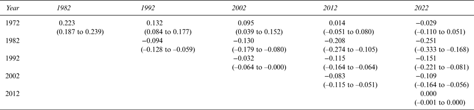
Table 3 Changes in Per Capita Wine Consumption (G Ethanol), 1972–2022, Population 15+

Table 4 Changes in Per Capita Spirits Consumption (G Ethanol), 1972–2022, Population 15+

Now consider the 1972 row for the beer table. The row tracks the changes through time, relative to 1972. So, the value in the 1972–1992 cell says that per capita ethanol consumption from beer in 1992 was 0.13 gallons higher than it was in 1972. The values in the remainder of the row have a similar interpretation. So, by reading across the 1972 row it can be seen that, on average, the initial increase in per capita beer consumption in the early part of the sample period, has, by 2012, been reversed.
The 2012–2022 cell in each table provides information on the expected change in the consumption level over the forecast period. The values suggest, on average, no change for beer and wine, but an increase in the consumption of spirits.
In Figure 4, for each beverage, the overall distribution of per capita consumption is shown, where the comparisons are for 1972 and 2012 (figures on the left); and 2012 and expected consumption in 2022 (figures on the right). For the spirits comparison the U-shape in dispersion can be clearly seen. Between 1972 and 2012 the distribution becomes much tighter, and then between 2012 and 2022 the distribution becomes more spread out again. The center of the distribution seems to shift back between 1972 and 2012, and then drift forward again for the forecast period. For wine we see both an increase in the mean and an increase in dispersion between 1972 and 2012, and little change for the forecast period. For beer the pattern is similar to spirits, but much less pronounced: a decrease in dispersion between 1972 and 2012 and then an increase in dispersion for the forecast period.

Figure 4 The Consumption Distribution: Past, Present, and Future
C. State Specific Information on Forecasts
In terms of specific states, in percentage terms, per capita spirits growth is forecast to be highest in: North Dakota, Iowa, Delaware, Oregon, and Idaho; per capita wine consumption growth is forecast to be highest in Delaware, West Virginia, Massachusetts, Idaho, and Tennessee; and for beer, per capita consumption growth is forecast to be highest in South Dakota, Kentucky, Ohio, Florida, Delaware, and Tennessee.
From a health policy and externality cost point of view, increases in per capita consumption are more concerning when the starting consumption level in a state is already high. As such, Table 5 identifies those states where the level of per capita consumption in 2012 was above the national average, and where further increases in consumption are forecast. In the table Delaware stands out as the only state where per capita consumption of all three beverage types is already above average, and where consumption is forecast to increase for all three beverages.
Table 5 Jurisdictions with above Average and Increasing Consumption

D. Policy Setting Comparison
The results for the comparison of tax rates are shown in Figure 5. In the figure, reading across the rows provides information on comparisons where the groups are held constant and beverage type varies; and reading down the columns provides comparisons where the beverage type is held constant and the group comparisons vary. The first row of the figure provides the comparisons between states where consumption is forecast to increase and consumption is forecast to decrease; the second row provides the comparisons of states where consumption is forecast to increase with states where consumption is forecast to remain unchanged; and the bottom row of the figure provides the comparisons of states where consumption is forecast to remain unchanged with states where consumption is forecast to decrease.
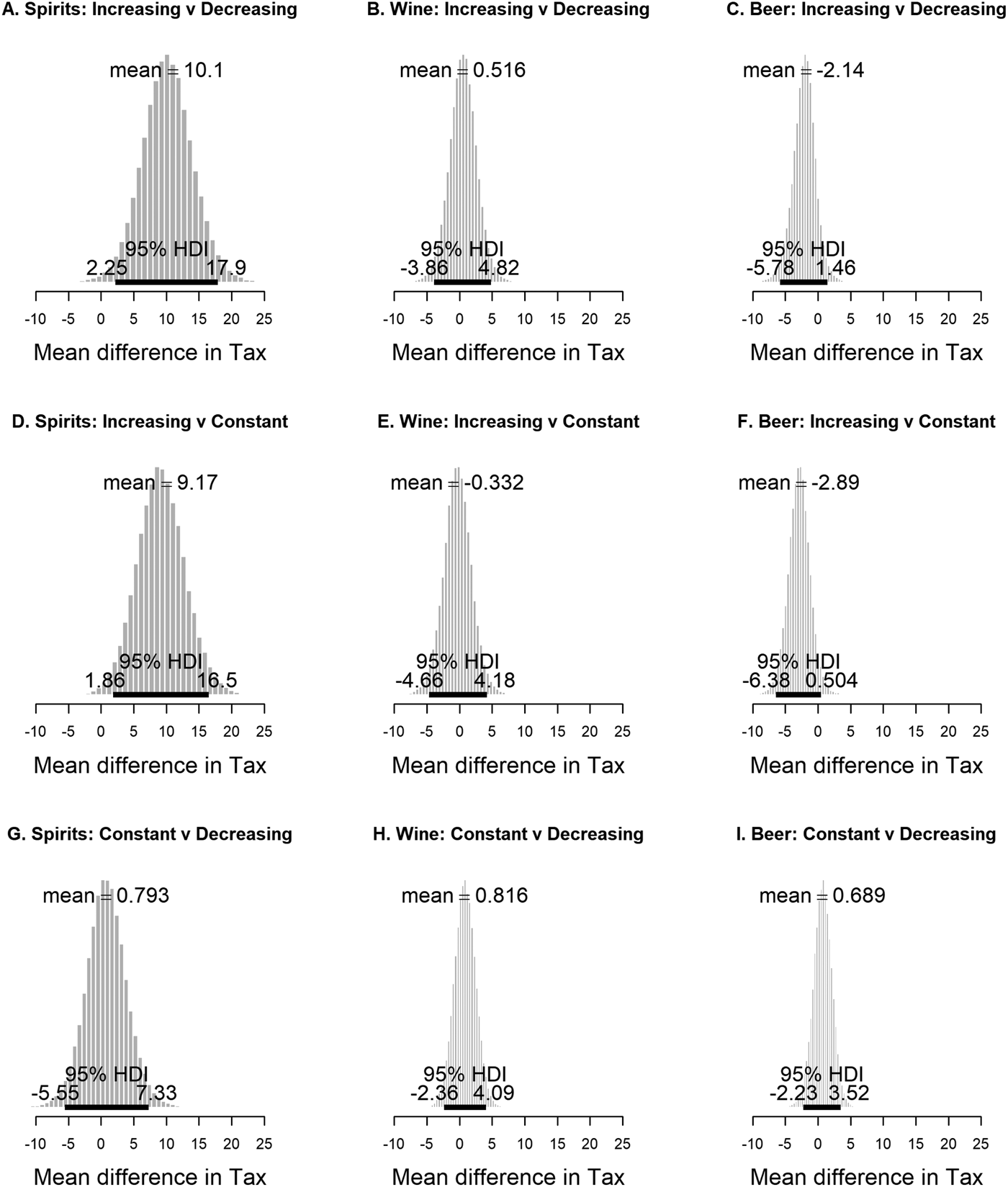
Figure 5 Comparison of Tax Settings by Consumption Forecast Grouping
For spirits the results suggest that taxes tend to be higher in jurisdictions where consumption is forecast to increase, compared to the jurisdiction where consumption is forecast to decrease or remain constant; and that there is no difference between jurisdictions where consumption is forecast to decrease and jurisdictions where consumption is forecast to remain constant. For wine, there is no evidence of any systematic differences across the three comparisons. For beer, taxes tend to be lower in jurisdictions where consumption is forecast to increase, relative to jurisdictions where consumption is forecast to increase or remain constant. Similar to spirits and wine, for beer, there appears to be no difference in taxes between jurisdictions where consumption is forecast to decrease and jurisdictions where consumption is forecast to remain constant.
The comparison of the policy settings by the three classifications is set out in Figure 6 and Table 6, and the visual is compelling. The figure clearly shows that there are no major systematic differences between the policy settings across jurisdictions with increasing, decreasing, or constant forecasts for future consumption. The values in Table 6 represent the proportion of policy setting variables in each category, and the 95% HDI. By reading across each row of the table it can be seen that there are no differences of any note.
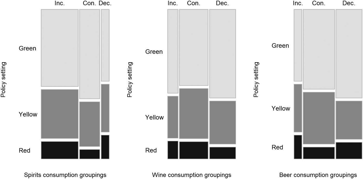
Figure 6 Comparison of Policy Settings
Table 6 Proportions Comparisons for Alcohol Policy Settings

IV. Discussion
There is global evidence of convergence in alcohol consumption patterns (Aizenman and Brooks, Reference Aizenman and Brooks2008; Colen and Swinnen, Reference Colen and Swinnen2016; Holmes and Anderson, Reference Holmes and Anderson2017; Smith and Solgaard, Reference Smith and Solgaard2000). The analysis presented here has found that since the early 1970s, within the United States, there was a clear trend towards increased convergence in both the level of consumption and the consumption mix for around 30 years, but that this trend has not been present since the early 2000s. Looking forward, forecasts of state level per capita consumption suggest a further increase in dispersion rather than convergence.
One way to characterize the consumption pattern of a nation is to identify a national beverage preference. In 2012, in no state was the ethanol share for wine or spirits greater than 45%, but beer accounted for at least 45% of consumption in 35 states. The beer ethanol share is actually above 50% in 24 states. At the end of the forecast period beer consumption is no longer quite so dominant, with the number of states where forecast beer consumption accounts for at least 45% of per capita consumption falling to 28 states, and the number of states where forecast beer consumption accounts for at least 50% of per capita consumption falling to 19 states. For wine, the forecasts suggest that by 2022 the consumption share will not have risen above 45% in any state. For spirits, the forecasts suggest that the consumption share will be above 45% in four states, and above 50% in two states by 2022. It therefore seems reasonable to describe the United States as a beer drinking nation, but one where beer's dominance is likely to fall over the coming decade.
For beer, it was found that jurisdictions where consumption was forecast to increase tended to have lower beer taxes than other jurisdictions. However, for wine, no relationship between tax rates and the forecast consumption change was identified. In the case of spirits, jurisdictions where consumption was forecast to increase were found to have higher spirits taxes than other jurisdictions. This finding was surprising as several review studies reported strong evidence that higher taxes are effective in lowering alcohol consumption and associated harms (Anderson, Chisholm, and Fuhr, Reference Anderson, Chisholm and Fuhr2009; Burton et al., Reference Burton, Henn, Lavoie, O'Connor and Perkins2017; Elder et al., Reference Elder, Lawrence, Ferguson and Naimi2010). It is, however, necessary to note that the associations identified here are correlations only, and do not identify causation. For example, a plausible hypothesis regarding spirits consumption could be that policy makers, seeing rising consumption as an issue, increase alcohol taxes. If this proposition is true, what we observe in the data are an association between higher taxes and growing consumption, but the relationship is one of higher consumption causing higher taxes, not higher taxes causing higher consumption. Also surprising was that no systematic relationship between the overall policy setting for alcohol and the consumption forecasts was observed, but this could be because the traffic light system for classifying policy settings was too coarse of a measure.
For the tax rate comparisons, it is also possible that the wrong comparison is being made. The comparison made in this research was between the forecast growth in consumption and the level of taxation. Recent work has shown that the real tax burden on alcohol beverages in the United States has been falling. For example, Naimi et al. (Reference Naimi, Blanchette, Xuan and Chaloupka2018) show that state alcohol excise taxes, in real terms, have fallen substantially since 1991 (the specific decreases are beer 30%, wine 27%, and spirits 32%). This decrease in the real tax rate means that real prices are falling, and hence consumption should rise. Further, the higher the level of the tax, the greater the real dollar value decline in the price of alcohol when taxes are not indexed to inflation. So, through time, the failure to index alcohol excise taxes results in greater real price falls (and hence consumption increases) for high tax beverages such as spirits. Although, more recent meta studies that correct for publication bias tend to find very inelastic demand (Nelson, Reference Nelson2013), and some studies that look explicitly at tax elasticity also find very little price responsiveness (Freeman, Reference Freeman2011).
Delaware was the only state identified where consumption of all three beverages was above the national average and consumption was also forecast to increase for each beverage. This suggests Delaware as a possible case study for further in-depth study. If, reflecting the evidence on externality costs discussed in the Introduction, greater emphasis is placed on controlling spirit and beer consumption, then there are 20 states where per capita consumption is already high, and either beer or spirit consumption is forecast to increase in the future. Of these states the District of Columbia and Florida stand out as states where the consumption of both beer and spirits is currently above average and forecast to increase. Although, in the case of the District of Columbia, it is possible that the spirits consumption data are impacted by cross-border sales issues. More generally, the identification of jurisdictions where consumption is both high and forecast to increase for at least one beverage type (Table 5) is valuable. These are states that can be prioritized for targeted work to identify the underlying causes of the increase.
The identification of states where consumption is currently low and forecast to decrease is also valuable, as in-depth study of these jurisdictions could also identify useful insights that have broader policy implications. The specific jurisdictions where consumption is currently low and consumption is forecast to fall for at least two beverage categories are: Arkansas (spirits, wine, and beer); Arizona (wine and beer); Kansas (spirits and beer), Nebraska (spirits and wine), and Oklahoma (spirits and beer).
V. Conclusion
This research has used a variety of techniques to describe the historical changes in alcohol consumption patterns at the U.S. state level and forecast future consumption. The analysis found that while there was a trend towards convergence for several decades, this trend was no longer present by the start of the century, and based on the forecasts, the return of a trend towards convergence is unlikely. No systematic correlations were found between alcohol taxes or other alcohol policy settings and forecast future consumption changes.
Appendix
Table A1 Model Summary Per Capita Beer Forecasts (Gallons (G) of Ethanol)

Table A2 Model Summary Per Capita Wine Forecasts (Gallons (G) of Ethanol)
Table A3 Model Summary Per Capita Spirits Forecasts (Gallons (G) of Ethanol)


