2.1 Description of the model

The self-consistent theory originates from the Reynolds decomposition of the velocity field into $\boldsymbol{U}(t)=\boldsymbol{U}_{m}+\boldsymbol{u}^{\prime }(t)$ , where $\boldsymbol{U}_{m}=\langle \boldsymbol{U}\rangle$ is the time-averaged mean velocity and $\boldsymbol{u}^{\prime }$ is the fluctuating velocity such that $\langle \boldsymbol{u}^{\prime }\rangle =0$ . Introducing $\boldsymbol{L}(\boldsymbol{U}_{m})$ as the Navier–Stokes operator linearized about the mean flow, substitution into (2.1) yields classical mean flow/fluctuation equations

defining the mean flow as a solution to the steady NSE, forced by the Reynolds stress of the fluctuation (i.e. the steady part of its nonlinear self-interaction) and the fluctuation as a solution to the NSE linearized about the mean flow, forced by the unsteady part of its nonlinear self-interaction.

In the self-consistent approach, the mean flow is not taken as a given, but comes instead as an output of a semi-linear approximation of (2.3) meant for the perturbation structure to be the one that forces the mean flow by its Reynolds stress in a manner such that the mean flow generates exactly the aforementioned perturbation. Expanding the perturbation into time-harmonic eigenmodes $\boldsymbol{u}$ of linear growth rate ${\it\sigma}$ and eigenfrequency ${\it\omega}$ , retaining the dominant eigenmode and forcing its growth rate to zero for the mean flow to be neutrally stable yields

where $\Vert \cdot \Vert$ is the norm induced by the $L^{2}$ inner product $(\cdot \mid \cdot )$ on the computational domain, $A$ is the real amplitude of the unit-norm eigenmode, ${\bf\psi}(\boldsymbol{u})=2\text{Re}\{\boldsymbol{u}^{\ast }\boldsymbol{\cdot }\boldsymbol{{\rm\nabla}}\boldsymbol{u}\}$ is the Reynolds stress divergence and $\text{Re}\{\cdot \}$ and * indicate respectively the real part and the conjugate of a complex quantity. The nonlinearity in $\boldsymbol{u}$ has been neglected in (2.3b ) because vortex shedding is assumed to be dominated by a single harmonic frequency.

This is the key difference with linear stability analyses featuring an eigenvalue problem identical to (2.4b ) on behalf of a small-amplitude assumption. If the nonlinearity is neglected in both (2.3a ) and (2.3b ), the approach is equivalent to classical stability analysis, as the mean flow reduces to the base flow $\boldsymbol{U}_{b}$ solution to the steady NSE

computed a priori and supposedly unaffected by the growth of unstable disturbances. Conversely, the approach reduces to mean flow stability analysis if the nonlinearity is neglected only in (2.3b ), but taken into account in (2.3a ), in which case the mean flow can be computed exactly a priori, averaging in time the instantaneous solution of a DNS of the NSE. There is however a certain lack of consistency in doing so because the Reynolds stress in (2.3a ) is that of the finite-amplitude vortex shedding coming from the DNS, not that of the small-amplitude eigenmode. According to Barkley (Reference Barkley2006), the results must be properly interpreted as applying in the case where the Reynolds stress itself is unperturbed at the order of the perturbation, thereby defining the so-called frozen Reynolds stress assumption.

2.2 Numerical methods

In the following, we obtain all semi-linear results relaxing the neutral stability condition and increasing the value of $A$ up to the point where ${\it\sigma}=0$ (which we assume is achieved to a sufficient degree when $|{\it\sigma}|\leqslant 10^{-6}$ ). For given amplitude, the self-consistent solutions are computed iteratively with a finite element method adapted from Meliga et al. (Reference Meliga, Boujo, Pujals and Gallaire2014), to which the reader is referred for further details. At each iteration, the mean flow is computed with the Newton–Raphson method, together with boundary conditions consisting of a uniform free stream at the inflow, symmetric conditions at the transverse boundaries and a stress-free outflow condition. The perturbation is computed with the Arnoldi method, together with boundary conditions linearized about the mean quantities. This repeats until the difference between two consecutive iterations of $\boldsymbol{U}_{m}$ is less than $10^{-12}$ in $L^{2}$ norm, which requires to under-relax the corrections made at each iteration.

In the following, we also report DNS results obtained using a second-order Crank–Nicholson scheme, with time step ${\rm\Delta}t=0.05$ . At the outflow, a more suitable advective condition is imposed, together with zero pressure at the upper-right corner of the domain. All simulations are carried out until the solution settles down to a periodic state, whereafter it is advanced in time over 500 time units (between 75 and 100 shedding cycles depending on the Reynolds number), sufficiently large to extract accurate frequency and amplitude information.

2.3 Uncontrolled flow

In this section, we briefly revisit the self-consistent modelling of the natural (uncontrolled) flow for validation purposes of our numerical tools. For various Reynolds numbers in the range $\mathit{Re}\leqslant 100$ , figure 1 reports limit-cycle frequency and amplitude results obtained using a mesh of the computational domain

made of 108 018 triangles (378 660 degrees of freedom), found to offer a good compromise between numerical accuracy and computational effort since numerical tests carried out at two other grid resolutions and spatial extents yield limited variations within 2 %. The semi-linear results reported as the open squares exhibit excellent agreement with the nonlinear values extracted from in-house DNS performed on the same mesh, shown as the open circles (note, DNS amplitudes are reported in terms of $\langle \Vert \boldsymbol{u}^{\prime }\Vert \rangle$ while self-consistent amplitudes are reported in terms of $A\sqrt{2}$ for the results to be comparable). At $Re=100$ , neutral stability is achieved for $A=2.2$ , or equivalently $A^{2}\Vert {\bf\psi}(\boldsymbol{u})\Vert /\Vert \boldsymbol{u}\Vert ^{2}=0.90$ , which matches well the amplitude of Mantič-Lugo et al. (Reference Mantič-Lugo, Arratia and Gallaire2014) obtained by normalizing the magnitude of the Reynolds stress instead of that of the eigenmode, and therefore validates the present computations. The associated self-consistent frequency ${\it\omega}=1.02$ ( $St={\it\omega}/2{\rm\pi}=0.162$ ) is very consistent with the value 1.03 predicted by the universal Strouhal–Reynolds relationship of Williamson (Reference Williamson1988) and with the mean flow stability results of Barkley (Reference Barkley2006). The spatial distribution of the self-consistent fields mean flow, fluctuation and Reynolds stress also agrees remarkably well with the DNS results (not shown here for conciseness).

Figure 1. Limit-cycle (a) frequency and (b) amplitude as a function of the Reynolds number: self-consistent (blue squares) versus DNS results (red circles). Open and filled symbols correspond respectively to the natural flow and to control with a secondary cylinder of diameter $d=0.1$ positioned at (a)  $\boldsymbol{x}_{c}=(1.2,1.0)$ and (b)  $\boldsymbol{x}_{c}=(0.8,1.6)$ . Experimental measurements from Williamson (Reference Williamson1988) (black line) and Strykowski & Sreenivasan (Reference Strykowski and Sreenivasan1990) (green crosses) are reported for comparison. The dash-dotted lines in (a) correspond to the frequency obtained by linear stability analysis of the base flow.

2.4 Relevance to vortex shedding control

It is the fundamental premise of our research that the self-consistent theory applies to controlled flows of practical interest. While this is a point that should be addressed on a case-by-case basis for arbitrarily large control amplitudes, we expect that it generally holds true for small to moderate amplitudes. As an illustration, we mimic here the approach of Strykowski & Sreenivasan (Reference Strykowski and Sreenivasan1990), insert a control cylinder of diameter $d=0.1$ at various positions in the flow and recompute the limit-cycle frequency and amplitude of the two-cylinder system using a mesh of the modified computational domain

obtained distributing 300 points at the surface of the control cylinder to accurately represent the flow (Meliga et al. Reference Meliga, Boujo, Pujals and Gallaire2014). For the positions $\boldsymbol{x}_{c}=(1.2,1.0)$ and $(0.8,1.6)$ considered, all mean flows are neutrally stable, while the shedding frequency is accurately predicted by the leading eigenfrequency (see figure 2 providing the results of linear stability analysis applied to the time-averaged mean flow), meaning that the controlled flows satisfy the real-zero imaginary-frequency (RZIF) property (Turton, Tuckerman & Barkley Reference Turton, Tuckerman and Barkley2015) and that the self-consistent theory does apply.

Figure 2. (a) Leading growth rate of the time-averaged mean flow as a function of the Reynolds number for control by a cylinder of diameter $d=0.1$ at $\boldsymbol{x}_{c}=(1.2,1.0)$ (upward triangles) and $\boldsymbol{x}_{c}=(0.8,1.6)$ (downward triangles). The leading growth rate of the base flow is shown for comparison as the dash-dotted lines. (b) Same as (a) for the leading eigenfrequency. The nonlinear frequency extracted from the DNS is indicated by the red circles.

Figure 3. (a) Self-consistent versus (b) time-averaged distribution of mean vorticity for control by a cylinder of diameter $d=0.1$ at $\boldsymbol{x}_{c}=(1.2,1.0)$ – $\mathit{Re}=100$ . (c,d) Same as (a,b) for the streamwise component of the Reynolds stress divergence.

The effect on the frequency is illustrated in figure 1(a) for the control cylinder placed at $\boldsymbol{x}_{c}=(1.2,1.0)$ . For this case, the critical Reynolds number is $\mathit{Re}_{c}=77.8$ (as predicted by linear stability analysis; see figure 2 a), whereupon the frequency is reduced by approximately 20 %. With the above key assumptions fulfilled, the self-consistent approach predicts accurately not only the frequency shift (as seen from the filled squares and circles showing the semi-linear and nonlinear results, respectively), but also the spatial structure of the controlled mean flow and Reynolds stresses, as documented in figure 3. In contrast, the leading eigenfrequency of the base flow (shown as the dashed line in figure 1 a) is completely out of range. The self-consistent results are also fully consistent with the experimental data of Strykowski & Sreenivasan (Reference Strykowski and Sreenivasan1990) pertaining to the same position of the control cylinder (reproduced as the cross symbols). There does exist a small quantitative difference, that we believe is attributable to a small bias in the experimental results, as the natural frequencies of Strykowski & Sreenivasan (Reference Strykowski and Sreenivasan1990) exhibit similar discrepancy with the reference data of Williamson (Reference Williamson1988) (shown as the black line). Figure 1(b) illustrates similarly the effect of the control cylinder placed at $\boldsymbol{x}_{c}=(0.8,1.6)$ on the amplitude. For this case, the critical Reynolds number is $\mathit{Re}_{c}=55$ , whereupon the self-consistent amplitude is reduced by approximately 30 %, the agreement between the self-consistent and the DNS results being again excellent.

These results provide clear evidence that the self-consistent theory captures well the effect of the control on the saturation mechanics. As could have been anticipated, different control positions yield markedly different effects on the frequency and the amplitude, for instance a control cylinder at $\boldsymbol{x}_{c}=(1.2,1.0)$ reduces the amplitude half as much as a control cylinder at $\boldsymbol{x}_{c}=(0.8,1.6)$ , while a control cylinder at $\boldsymbol{x}_{c}=(0.8,1.6)$ barely affects the frequency (not shown here). This stresses the need to explore the parameter space for an efficient control design, an investigation from now on performed in a systematic way using sensitivity analysis, as further developed in §§ 3 and 4.

3.1 Theoretical framework

In the limit of infinitesimal control amplitudes, the linear estimate of the limit-cycle frequency variation can be expressed as the inner product between the control forces and sensitivity functions representing the variational derivatives of the frequency to sources of momentum in the flow. This amounts to invoking the first-order Taylor expansion around zero of ${\it\omega}$ viewed as a function of $\boldsymbol{F}$ and $\boldsymbol{f}$ , given that only the sensitivity, not the variation, depends on the choice of the inner product structure. We derive here an analytical expression of the sensitivity functions $\boldsymbol{{\rm\nabla}}_{\boldsymbol{F}}{\it\omega}$ and $\boldsymbol{{\rm\nabla}}_{\boldsymbol{f}}{\it\omega}$ such that

using a variational technique based on the computation of Lagrange multipliers. We use the body forces $\{\boldsymbol{F},\boldsymbol{f}\}$ as control variables, the self-consistent quantities $\{\boldsymbol{U}_{m},\boldsymbol{u},{\it\sigma},{\it\omega},A\}$ as state (or direct) variables, introduce Lagrange multipliers $\{\boldsymbol{U}^{\dagger },\boldsymbol{u}^{\dagger },{\it\alpha}^{\dagger },{\it\beta}^{\dagger }\}$ (also termed co-state or adjoint variables) and define the functional

whose gradient with respect to any variable $\boldsymbol{s}$ is

The adjoint fluctuation $\boldsymbol{u}^{\dagger }$ is complex, while the adjoint mean flow $\boldsymbol{U}^{\dagger }$ and the adjoint scalar parameters ${\it\alpha}^{\dagger }$ (ensuring neutral stability) and ${\it\beta}^{\dagger }$ (ensuring unit norm of the eigenmode) are real, which results in $\mathscr{L}$ being real as well.

Assuming all partial derivatives with respect to the direct and adjoint variables to be zero $(\partial \mathscr{L}/\partial \boldsymbol{U}_{m}=\cdots \partial \mathscr{L}/\partial {\it\beta}^{\dagger }=0)$ , the total variation of the Lagrangian reads

where the last equality follows from the derivatives with respect to the adjoint variables being zero, which ensures that the direct variables are solutions to the self-consistent system (3.1) and that the Lagrangian reduces to the limit-cycle frequency $(\mathscr{L}={\it\omega})$ . Comparing relations (3.3) and (3.6), the sensitivities are deduced as

Using integration by parts to cancel the partial derivatives with respect to the direct variables, the adjoint variables come as the solutions to the self-consistent system

where $\boldsymbol{L}^{\dagger }$ is the adjoint of the linearized Navier–Stokes operator. At this stage, a compatibility condition must be enforced to guarantee the existence of a solution to the adjoint fluctuation equation (3.8b ). This is because there exists a non-trivial solution to

for ${\it\sigma}=0$ and ${\it\omega}$ equal to the limit-cycle frequency, on behalf of $\boldsymbol{u}$ being a solution to eigenvalue problem (2.4b ). Said condition is derived by taking the inner product of (3.8b ) with the eigenmode $\boldsymbol{u}$ and integrating by parts the left-hand side, which yields

since the operators are by definition such that $(\boldsymbol{u}^{\dagger }\mid \boldsymbol{L}(\boldsymbol{U}_{m})\boldsymbol{u})=(\boldsymbol{L}^{\dagger }(\boldsymbol{U}_{m})\boldsymbol{u}^{\dagger }\mid \boldsymbol{u})$ . Further integrating by parts the first term in the right-hand side and retaining the real part, we obtain

and ultimately

using (3.8d ). Since we investigate the sensitivity of the natural limit cycle ( $\boldsymbol{f}=\mathbf{0}$ ), the self-consistent adjoint system reduces to

Both problems (3.13a )–(3.13b ) for the adjoint mean flow and fluctuation must be solved simultaneously, together with normalisation condition (3.13c ) and compatibility condition (3.13d ). The boundary conditions are such that the bilinear concomitant arising on the outer boundary of the domain during the integration by parts is zero, which yields classical homogeneous conditions at the inflow, symmetric conditions at the transverse boundaries and an adjoint stress-free outflow condition (Marquet et al. Reference Marquet, Sipp and Jacquin2008a ).

Since system (3.13) is independent of time, we obtain the adjoint fields $\boldsymbol{U}^{\dagger }$ and $\boldsymbol{u}^{\dagger }$ and the adjoint parameter ${\it\alpha}^{\dagger }$ using an iterative method detailed in appendix A.1. Suffice it to say that convergence is achieved within a few tens of iterations, which takes less than an hour on a regular sequential workstation. The computational cost is thus essentially that of solving the self-consistent system of the uncontrolled flow, which is less than that of performing the DNS on the same mesh in the range of Reynolds number considered herein (by more than 80 % at $Re=60$ and approximately 50 % at $Re=100$ ). The sensitivity of the limit-cycle frequency to a steady control force ( $\boldsymbol{{\rm\nabla}}_{\boldsymbol{F}}{\it\omega}=\boldsymbol{U}^{\dagger }$ , physically representing the self-consistent approximation to the mean component of the time-dependent sensitivity computed by Luchini et al. (Reference Luchini, Giannetti, Pralits, Braza and Hourigan2009)) is presented in figure 4(a) at $Re=100$ . Streamlines of the underlying vector field give the local orientation of the gradient and colour levels indicate its magnitude. In practice, a local steady force ${\bf\delta}\boldsymbol{F}$ oriented in the same direction (respectively, in the opposite direction) as the arrows plotted in figure 4(a) therefore increases (respectively, decreases) the frequency by a quantity proportional to the local magnitude. The regions of highest sensitivity are located on either side of the cylinder, at the periphery of the mean recirculating streamline (shown as the dashed line) and in the inner recirculation region, close to $\boldsymbol{x}=(1,0)$ . Conversely, the sensitivity to an oscillating control force ( $\boldsymbol{{\rm\nabla}}_{\boldsymbol{f}}{\it\omega}=\boldsymbol{u}^{\dagger }$ , physically representing the self-consistent approximation to the fluctuating component of the time-dependent sensitivity computed by Luchini et al. (Reference Luchini, Giannetti, Pralits, Braza and Hourigan2009)) shown in figure 4(b) (with no streamlines since the underlying vector field is complex) is concentrated close to the mean separation points and in the shear layers.

Figure 4. Self-consistent sensitivity of the limit-cycle frequency – $\mathit{Re}=100$ . The magnitude of sensitivity is given by the colour levels and the orientation of the underlying vector by the superimposed streamlines. (a) Sensitivity to a steady force $(\boldsymbol{{\rm\nabla}}_{\boldsymbol{F}}{\it\omega}=\boldsymbol{U}^{\dagger })$ . (b) Sensitivity to an unsteady force fluctuating at the fundamental frequency $(\boldsymbol{{\rm\nabla}}_{\boldsymbol{f}}{\it\omega}=\boldsymbol{u}^{\dagger })$ . Note the different colour look-up tables in (a) and (b).

Relation (3.7) carries over to the base and mean flow approaches, provided the adjoint fields are redefined as the solutions to

with $\boldsymbol{U}$ being either the base flow or the time-averaged mean flow obtained by DNS. System (3.14) is termed uncoupled because the eigenvalue problem for the adjoint fluctuation can be solved first, and then the computed solution can be used to solve the adjoint mean flow equation. The sensitivity fields obtained by doing so are however markedly different from their self-consistent counterparts, as can be seen comparing figures 4 and 5. Both the base and mean flow approaches somehow end up providing a rough approximation of the fluctuating component $\boldsymbol{{\rm\nabla}}_{\boldsymbol{f}}{\it\omega}$ , although the base flow approach overestimates the size of the sensitive regions and the mean flow approach overestimates the level of sensitivity in the vicinity of the separation points. The discrepancy is more obvious looking at the mean component $\boldsymbol{{\rm\nabla}}_{\boldsymbol{F}}{\it\omega}$ , as the base flow approach misses completely on the location and spatial extension of the sensitive regions (not to mention the level of sensitivity in these regions), while the mean flow approach manages to predict, albeit approximately, the location and spatial extension of the primary sensitive regions. Such results clearly stress that an accurate description of the nonlinear mean flow/fluctuation is mandatory to obtain proper sensitivity predictions, as further discussed in § 3.2.

Figure 5. Same as figure 4 for the sensitivities computed in the frame of the (a,b) base flow approach and of the (c,d) mean flow approach – $\mathit{Re}=100$ . The colour look-up table is identical to that used in figure 4.

Figure 6. Variation of the limit-cycle frequency induced by the localized feedback defined by (3.15) – $\mathit{Re}=100$ . Solid lines indicate linear predictions computed in the frame of the sensitivity analysis from (3.17). The dashed and dash-dotted lines denote the results obtained by the mean and the base flow approaches, respectively. (a)  $\boldsymbol{x}_{c}=(1.6,0.5)$ . (b)  $\boldsymbol{x}_{c}=(1.0,0.8)$ . (c)  $\boldsymbol{x}_{c}=(0.0,0.6)$ . (d)  $\boldsymbol{x}_{c}=(1.5,0.0)$ .

3.2 Effect of a localized feedback, wavemaker

In this section, we consider the effect of a ‘force–velocity’ coupling under the form of a steady force proportional to the mean velocity and a fluctuating force proportional to the eigenmode velocity. If spatially localized, such a forcing can also be viewed as a feedback induced by an actuator located at the same station $\boldsymbol{x}_{c}$ as the sensor. Both force components can be expressed as

where ${\it\delta}(\boldsymbol{x})$ stands for the 2-D Dirac delta function, $b_{1,2}$ is the amplitude of the feedback and the frequency variation follows straightforwardly as

The Reynolds number is set to $\mathit{Re}=100$ in the remainder of the section. For several locations of the feedback force, figure 6 compares the linear variation ${\it\delta}{\it\omega}$ of the limit-cycle frequency computed in the frame of the present self-consistent sensitivity analysis (red lines), whose correctness and numerical accuracy is carefully assessed in appendix A.2, to those obtained by the mean and base flow approaches (dashed and dash-dotted lines). To do so, all delta functions are smoothed out numerically into Gaussians; see Meliga et al. (Reference Meliga, Boujo, Pujals and Gallaire2014) for proof of relevance. For the positions $\boldsymbol{x}_{c}=(1.6,0.5)$ and $\boldsymbol{x}_{c}=(1.0,0.8)$ documented in figure 6(a,b), the base flow approach underestimates considerably the frequency variations, which is not too surprising since it even fails to provide a correct estimation of the uncontrolled limit-cycle frequency. The mean flow approach provides a better overall estimation at $\boldsymbol{x}_{c}=(1.0,0.8)$ because the position is not too far downstream, in a region where the mean flow velocity is large and the Reynolds stress is weak. In contrast, at $\boldsymbol{x}_{c}=(1.6,0.5)$ the Reynolds stress is large, and the variation is underestimated by approximately 25 %. Looking at the individual variations caused by the mean and fluctuating components of the feedback unveils the fact that both contributions are actually miscalculated but the errors somehow compensate one another (not shown here), meaning the overall comparison is actually worse than it looks. Other comparisons documented in figures 6(c,d) add to the proof that overlooking the effect of the control on the Reynolds stress (and its subsequent feedback onto the mean flow) can lead to flawed theoretical predictions, for instance the mean flow approach overestimates the overall variation achieved at $\boldsymbol{x}_{c}=(0.0,0.6)$ by more than 100 %, while it squarely fails to predict the sign of that variation achieved at $\boldsymbol{x}_{c}=(1.5,0.0)$ .

Figure 7. Sensitivity of the limit-cycle frequency to a localized feedback as quantified by the products (a)  $\Vert \boldsymbol{U}^{\dagger }(\boldsymbol{x}_{c})\Vert \boldsymbol{\cdot }\Vert \boldsymbol{U}_{m}(\boldsymbol{x}_{c})\Vert$ and (b)  $2A\Vert \boldsymbol{u}^{\dagger }(\boldsymbol{x}_{c})\Vert \boldsymbol{\cdot }\Vert \boldsymbol{u}(\boldsymbol{x}_{c})\Vert$ , representing respectively the contributions of the mean and fluctuating feedback force to the wavemaker.

A bound for the frequency variation induced by the present feedback force can be obtained applying classical Cauchy–Schwartz and triangular inequalities to the right-hand side of (3.17), which yields

Equation (3.18) readily expresses that ${\it\delta}{\it\omega}$ is non-vanishing only in the flow region where the product of the modulus of the self-consistent direct and adjoint fields is not zero. The associated overlapping region can thus be considered as the ‘wavemaker’ responsible for the selection of the nonlinear frequency, thereby extending the concept introduced by Giannetti & Luchini (Reference Giannetti and Luchini2007) for the leading eigenvalue of the unstable base flow. We show in figure 7(a) the spatial distribution of the product $\Vert \boldsymbol{U}^{\dagger }(\boldsymbol{x}_{c})\Vert \boldsymbol{\cdot }\Vert \boldsymbol{U}_{m}(\boldsymbol{x}_{c})\Vert$ obtained for $(b_{1},b_{2})=(1,0)$ and physically representing the contribution of the mean feedback. It is almost zero downstream, but exhibits large magnitudes on either side of the mean recirculation region and also further upstream, offset from the centreline. In contrast, the magnitude of the product $2A\Vert \boldsymbol{u}^{\dagger }(\boldsymbol{x}_{c})\Vert \boldsymbol{\cdot }\Vert \boldsymbol{u}(\boldsymbol{x}_{c})\Vert$ shown in figure 7(b) for $(b_{1},b_{2})=(0,1)$ and physically representing the contribution of the fluctuating feedback is almost zero everywhere, except in two lobes located symmetrically across the recirculation region. This is due to the convective non-normality of the NSE transporting all direct fluctuations downstream and all adjoint fluctuations upstream (Chomaz Reference Chomaz2005). Both components of the force therefore sign distinct wavemaker regions, which is consistent with the results of figure 4, but the latter regions differ from those exhibiting only large sensitivity since the amplitude of the direct fields and their orientation with respect to the sensitivities also come into it. Note, a similar wavemaker region has been identified by Luchini et al. (Reference Luchini, Giannetti, Pralits, Braza and Hourigan2009) from the average in time of the exact product between the time-dependent sensitivity and feedback force, whose self-consistent equivalent is obtained adding up the above products for $|b_{1}|=|b_{2}|$ . We have checked that almost identical results are obtained doing so, but choose not to discuss this further because the present results depend on the ratio of $|b_{1}|/|b_{2}|$ , so the interpretation would in some sense lack generality.

3.3 Application to control by a small circular cylinder

We now use knowledge of the sensitivity as a systematic guideline on where to insert a small device in the attempt to modify the limit-cycle frequency. This can be of practical interest for fluid-induced vibration problems because the only dangerous flow instabilities are those whose frequencies match the frequencies of the structural eigenmodes, meaning that shifting the threatening flow frequencies can be sufficient to prevent the onset of synchronized regimes. Following Hill (Reference Hill1992), the presence of a small control cylinder at given position $\boldsymbol{x}_{c}$ is modelled by the force it exerts on the flow, defined conveniently as the pointwise reacting force localized at the same location where the control cylinder is placed, equal and opposite to the force that would act on a fictitious cylinder of same diameter invested by a uniform flow at the local velocity. We build here on previous studies focusing on steady and unsteady effects modelling the presence of the control cylinder (Giannetti & Luchini Reference Giannetti and Luchini2007; Marquet et al. Reference Marquet, Sipp and Jacquin2008a ,Reference Marquet, Sipp, Jacquin and Chomaz b ; Meliga et al. Reference Meliga, Sipp and Chomaz2010, Reference Meliga, Boujo, Pujals and Gallaire2014), and decompose the latter force into steady and fluctuating components reading

where $C_{d}$ is the drag coefficient of the control cylinder and $|\cdot |$ denotes the norm induced by the dot product. The frequency variation follows straightforwardly as

Of course, this cylinder force model stands as a first approximation derived in the limit of small control cylinders. On the one hand, it assumes the diameter of the control cylinder to be much smaller than the local inhomogeneity length scale, which results on the force acting on the control cylinder being pure drag (as a non-uniform flow would otherwise exert an additional lift force proportional to the local shear). On the other hand, it assumes negligible inertia effects and thus the force acting on the cylinder at each time instant to be identical to the force that would act if the upstream flow at the same instant was a steady one (quasi-static assumption). This in particular is expected to hold because the advection time scale in the vicinity of the control cylinder is much smaller than the vortex shedding period, a regime where the drag coefficient $C_{d}$ is essentially equal to its value for steady flow, and thus depends only on the local Reynolds number $\mathit{Re}_{d}(\boldsymbol{x}_{c})=|\boldsymbol{U}_{m}(\boldsymbol{x}_{c})|d/{\it\nu}$ . The model also assumes the fluctuating force to be harmonic at the fundamental frequency while overlooking the effect of the higher harmonics, which is expected to hold as long as a self-consistent description of the controlled flow remains relevant. We show in the following that even such a basic modelling can guide appropriate placement of the control cylinder in the sense that the localization of the sensitive regions can be safely inferred with good accuracy despite the not-so-high degree of approximation used to represent the control cylinder itself.

Figure 8. Variation of the limit-cycle frequency induced by a control cylinder of diameter $d=0.1$ whose presence is modelled by (3.19) – $\mathit{Re}=100$ . The circle symbol marks the position $\boldsymbol{x}_{c}=(1.2,1.0)$ for which theoretical predictions are compared to self-consistent and DNS results of open-loop control by a small control cylinder in figures 1(a) and 10.

Figure 9. Same as figure 8 for the individual variations computed retaining the (a) mean and (b) fluctuating components of the model force. The map in figure 8 is thus retrieved as the sum of these two maps.

We show in figure 8 a map of the variation of the limit-cycle frequency ${\it\delta}{\it\omega}$ induced by a control cylinder of diameter $d=0.1$ at $\mathit{Re}=100$ , for which the local Reynolds number is below 10 and the drag coefficient $C_{d}$ is approximated using the three-parameter power law defined in Meliga et al. (Reference Meliga, Boujo, Pujals and Gallaire2014). It exhibits only negative variations (as indicated by the blue hue) corresponding to a decrease of the frequency, the maximum effect being achieved in a region originating from the shear layers and surrounding the mean recirculating streamline. Weaker yet significant decrease is noticeable further upstream, offset from the centreline. The maps of the individual variations obtained retaining either the mean or the fluctuating component of the force, shown in figure 9, suggest that it is the mean force (respectively the fluctuating force) that triggers the frequency decrease observed on either side of the mean recirculation region and upstream of the cylinder (respectively in the rear of the recirculation region). The fluctuating force is seen to additionally increase the limit-cycle frequency just upstream of the separation points (red hue), but not sufficiently to compensate for the large decrease induced by the mean force at this location, hence the overall frequency reduction in figure 8. All in all, the mean force produces larger variations, but because of this disjointedness in the sensitive regions, the dominant contribution can be driven by either component, depending on the location of the control cylinder.

Figure 10. Limit-cycle frequency as a function of the Reynolds number for control by a cylinder of diameter (a)  $d=0.1$ and (b)  $d=0.02$ at $\boldsymbol{x}_{c}=(1.2,1.0)$ . Linear sensitivity predictions are shown as the small circle symbols, with dark and light blue shades used to decompose into the contributions of the mean and fluctuating components of the model force. Semi-linear and nonlinear data are also reproduced from figure 1 as the various square/circle symbols.

We return now to the experimental results of Strykowski & Sreenivasan (Reference Strykowski and Sreenivasan1990), whom we recall report a control cylinder of diameter $d=0.1$ placed at $\boldsymbol{x}_{c}=(1.2,1.0)$ to suppress vortex shedding for $\mathit{Re}<80$ and to reduce the oscillation frequency by approximately 30 % afterwards. In figure 10(a), we report the various semi-linear (blue) and nonlinear (red) data used in figure 1(a) to evidence that this effect is well captured by the self-consistent theory. We now use blue shades to superimpose the effect of the control cylinder, as theoretically predicted from (3.20), with the dark (respectively light) blue shade representing the effect of the mean (respectively the fluctuating) component of the model force. For this position, marked by the grey circle in figure 8, both components contribute significantly to the frequency reduction, with the variation induced by the mean force being approximately twice as large as that induced by its fluctuating counterpart. The theoretical results exhibit a satisfactory agreement with the semi-linear and nonlinear data, meaning that the approach provides both qualitative and quantitative predictions. There does exist a discrepancy that we attribute to our cylinder force model being excessively simple for such a non-small control cylinder, as the agreement is almost perfect in figure 10(b) reporting the same results for a smaller control cylinder of diameter $d=0.02$ .

4.1 Theoretical framework

We analyse now similarly the effect of the control upon the limit-cycle amplitude. No comparison is made with the base and mean flow approaches, since those are simply unable to predict the saturation amplitude. In the following, we ease the presentation of the theoretical framework using the squared amplitude $A^{2}$ (physically representing the amplitude of the Reynolds stress in the mean flow equation) as a convenient direct variable. An analytical expression of the sensitivity functions $\boldsymbol{{\rm\nabla}}_{\boldsymbol{F}}A^{2}$ and $\boldsymbol{{\rm\nabla}}_{\boldsymbol{f}}A^{2}$ , such that

is derived following the same steps as in § 3.1 to express the total variation of the Lagrangian

We deduce the sensitivities as

where the adjoint fields come as solutions to the new self-consistent system

formally similar to that (3.13) governing the sensitivity of the limit-cycle frequency, but featuring an additional forcing term in the adjoint fluctuation equation (4.4b ). Again, a compatibility condition must be enforced to guarantee the existence of a solution, which is achieved by taking the inner product of (3.8b ) with the eigenmode $\boldsymbol{u}$ , integrating by parts and retaining the real part. This yields the same relation

as in § 3.1, except that it reduces now to

using (4.4d ). Since we investigate the sensitivity of the natural limit cycle ( $\boldsymbol{f}=\mathbf{0}$ ), the self-consistent adjoint system reads ultimately

The boundary conditions to be used are those defined in § 3.1, namely homogeneous conditions at the inflow, symmetric conditions at the transverse boundaries and adjoint stress-free conditions at the outflow.

The numerical method used to compute all adjoint quantities of interest is presented in appendix B.1, together with validation data documented in appendix B.2. The sensitivity of the limit-cycle amplitude to a steady control force $(\boldsymbol{{\rm\nabla}}_{\boldsymbol{F}}A^{2}=\boldsymbol{U}^{\dagger })$ shown in figure 11(a) at $\mathit{Re}=100$ exhibits large magnitudes close to the cylinder, at the mean separating points, as well as in the inner recirculation region, close to the centreline, which constitute noticeable differences with respect to the frequency; see figure 4(a). In contrast, the sensitivity to an oscillating control force $(\boldsymbol{{\rm\nabla}}_{\boldsymbol{f}}A^{2}=\boldsymbol{u}^{\dagger })$ shown at the same Reynolds number in figure 11(b) is the largest close to the separation points and (in a lesser extent) in the inner recirculation region, i.e. the same regions where the frequency is most sensitive; see figure 4(b).

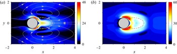
Figure 11. Self-consistent sensitivity of the limit-cycle amplitude – $\mathit{Re}=100$ . The magnitude of sensitivity is given by the colour levels and the orientation of the underlying vector by the superimposed streamlines. (a) Sensitivity to a steady force $(\boldsymbol{{\rm\nabla}}_{\boldsymbol{F}}A^{2}=\boldsymbol{U}^{\dagger })$ . (b) Sensitivity to an unsteady force fluctuating at the fundamental frequency $(\boldsymbol{{\rm\nabla}}_{\boldsymbol{f}}A^{2}=\boldsymbol{u}^{\dagger })$ .

Figure 12. Sensitivity of the limit-cycle amplitude to a localized feedback as quantified by the products (a)  $\Vert \boldsymbol{U}^{\dagger }(\boldsymbol{x}_{c})\Vert \boldsymbol{\cdot }\Vert \boldsymbol{U}_{m}(\boldsymbol{x}_{c})\Vert$ and (b)  $2A\Vert \boldsymbol{u}^{\dagger }(\boldsymbol{x}_{c})\Vert \boldsymbol{\cdot }\Vert \boldsymbol{u}(\boldsymbol{x}_{c})\Vert$ , representing respectively the contributions of the mean and fluctuating feedback force to the wavemaker – $\mathit{Re}=100$ .

4.2 Effect of a localized feedback, wavemaker

We return here to the localized feedback force (3.15) introduced in § 3.2, and present in figure 12 the spatial distribution of the overlapping regions between the self-consistent direct and adjoint fields, considered as the ‘wavemaker’ of the instability, responsible for the selection of the oscillation amplitude. All results are provided for a Reynolds number $\mathit{Re}=100$ . In figure 12(a), we show the spatial distribution of the product $\Vert \boldsymbol{U}^{\dagger }(\boldsymbol{x}_{c})\Vert \boldsymbol{\cdot }\Vert \boldsymbol{U}_{m}(\boldsymbol{x}_{c})\Vert$ representing the contribution of the mean feedback, whose amplitude is large in the vicinity of the mean separating points, and also moving away from the cylinder surface in the cross-wise direction. In contrast, the magnitude of the product $2A\Vert \boldsymbol{u}^{\dagger }(\boldsymbol{x}_{c})\Vert \boldsymbol{\cdot }\Vert \boldsymbol{u}(\boldsymbol{x}_{c})\Vert$ shown in figure 12(b) and representing the contribution of the fluctuating feedback is large in the rear part of the recirculation region, and in the near wake, meaning that both components of the force again sign distinct wavemaker regions.

Figure 13. Variation of the limit-cycle amplitude induced by a control cylinder of diameter $d=0.1$ – $\mathit{Re}=100$ . The grey circles mark the positions $\boldsymbol{x}_{c}=(0.8,1.6)$ and $(1.0,0.7)$ for which theoretical predictions are compared to self-consistent and DNS results of open-loop control by a small control cylinder in figures 1(b) and 15.

Figure 14. Same as figure 13 for the individual variations computed retaining the (a) mean and (b) fluctuating components of the model force.

4.3 Control by a small circular cylinder

We use now the sensitivity as a systematic path to guide the best positions for placement of a control cylinder in view of alleviating the shedding activity. We show in figure 13 a map of the variation of the limit-cycle amplitude ${\it\delta}A^{2}$ induced by a control cylinder of diameter $d=0.1$ at $\mathit{Re}=100$ . Interestingly, the control cylinder can increase or decrease the amplitude (while it has been shown to decrease exclusively the frequency in § 3.3), as illustrated by the positive (respectively negative) variations prevailing on either side of the cylinder and of the mean recirculating streamline (respectively in the rear part of the recirculation and on either side of the recirculation up to the potential flow). Both components of the force act in different flow regions, as seen from figure 14 showing maps of the individual variations obtained retaining either the mean or the fluctuating component of the force. Only the reduction of the amplitude found in the rear part of the recirculation is ascribed to the fluctuating component, while all other variations are essentially driven by the mean force. The fluctuating force also decreases the limit-cycle amplitude in the near-wake region, but this effect is almost exactly counter-balanced by the increase induced by the mean force, hence the absence of any variation in this region in figure 13.

Figure 15. (a,b) Limit-cycle amplitude as a function of the Reynolds number for control by a cylinder of diameter (a)  $d=0.1$ and (b)  $d=0.02$ at $\boldsymbol{x}_{c}=(0.8,1.6)$ . Linear sensitivity predictions are shown as the small circular symbols, with dark and light blue shades used to decompose into the contributions of the mean and fluctuating components of the model force. Semi-linear and nonlinear data are also reproduced from figure 1 as the various square/circle symbols. (c,d) Same as (a,b) for a control cylinder at $\boldsymbol{x}_{c}=(1.0,0.7)$ .

In figure 15(a), we report the various semi-linear and nonlinear data used in figure 1(b) to evidence that the present self-consistent approach predicts well the reduction of the fluctuation amplitude achieved placing a control cylinder of diameter $d=0.1$ at $\boldsymbol{x}_{c}=(0.8,1.6)$ . As in figure 10, we use blue shades to superimpose the effect of the control cylinder as predicted in the frame of the current sensitivity analysis, with the dark (respectively light) blue shade representing the effect of the mean (respectively the fluctuating) component of the model force. For this position, only the dark blue shade is visible, as the contribution of the fluctuating component is negligible, consistent with the results of figure 13. Again, the theoretical results exhibit a good agreement with the semi-linear and nonlinear data, meaning that the approach provides both qualitative and quantitative predictions despite the small discrepancy due to the non-smallness of the control cylinder (see the improved agreement in figure 15(b) showing the exact same results for $d=0.02$ ).

Similar results are presented in figure 15(c,d) for a control cylinder at $\boldsymbol{x}_{c}=(1,0.7)$ , which is a challenging case to be recovered by sensitivity analysis because both components of the force yield significant effects that end up cancelling each other out, hence resulting in little overall variation of the amplitude. Still, we observe a good agreement between the linear and semi-linear results, at least for values of $Re$ not too close to the instability threshold. The discrepancy observed in the vicinity of $\mathit{Re}_{c}$ however raises questions regarding the ability of the approach in identifying those flow regions where the control cylinder completely suppresses vortex shedding. Since the growth rate is forced to zero in the present formulation, it seems natural to correlate such a quenching of the instability to zero limit-cycle amplitude. For a control cylinder of diameter $d=0.1$ , we show in figure 16 the loci of all points in the $(x,y)$ -plane corresponding to such zero controlled amplitude, calculated at several Reynolds numbers as the isocontours of ${\it\delta}A^{2}=-A^{2}$ . In the range $\mathit{Re}<50$ , vortex shedding is suppressed by placing the control cylinder either in the outer region or within the recirculation region, close to the centreline. This secondary region vanishes as the Reynolds number increases, while the spatial extent of the outer region reduces until it vanishes as well at $\mathit{Re}=52$ . This behaviour is qualitatively consistent with the results of Strykowski & Sreenivasan (Reference Strykowski and Sreenivasan1990) – see the figure 20 therein – but there exist noticeable quantitative differences, since these authors report full restabilization of the flow up to $\mathit{Re}\sim 80$ .

Figure 16. Loci of all points in the $(x,y)$ -plane corresponding to zero controlled amplitude for a control cylinder of diameter $d=0.1$ , obtained at several Reynolds numbers from the sensitivity functions as the isocontours of ${\it\delta}A^{2}=-A^{2}$ .

Part of the explanation lies in the linear nature of sensitivity methods, whose accuracy is inherently limited by the finite control amplitude needed to stabilize the flow. This can be perilous close to the instability threshold, where the amplitude varies very nonlinearly with $Re$ (for such a Hopf bifurcation, it varies as the square root of the departure from criticality, opposite to the growth rate which varies linearly). Small inaccuracy in the theoretical model may thus yield a non-small discrepancy with the semi-linear results, such miscalculations being clearly visible in figure 15(a,c), and leading to the related instability thresholds being underestimated by 10 % for both positions considered. Assuming this trend carries over to other positions, this makes the predicted stabilizing regions smaller than they ought to be, consistent with the results of figure 16. Another part of the explanation lies in the correlation between suppression of vortex shedding and zero limit-cycle amplitude. Indeed, figure 17(a), pertaining to a control cylinder located at $\boldsymbol{x}_{c}=(1.2,1.0)$ , shows that the control affects not only the threshold of instability, but also the structure of the bifurcation, with a small diameter $d=0.02$ yielding a classical supercritical bifurcation, but the larger diameter $d=0.1$ yielding an unexpected subcritical bifurcation (which has been assessed rigorously from DNS calculations and from weakly nonlinear analysis, besides the present self-consistent results). This is because the induced mean flow distortion is destabilizing for small amplitudes of the eigenmode amplitude. This is best seen from the evolution of ${\it\sigma}$ as the amplitude $A$ is increased from zero in figure 17(b), where the base flow is initially turned into an increasingly unstable mean flow. For sufficiently large amplitudes $A\gtrsim 0.7$ , the nonlinearity becomes stabilizing again and the mean flow is increasingly stabilized, up to the point where neutral stability is achieved. In contrast, for $d=0.02$ , the mean flow distortion is exclusively stabilizing and the growth rate decreases monotonically to zero. Such an effect is local in the sense that for the same diameter $d=0.1$ , the bifurcation remains supercritical at both positions $\boldsymbol{x}_{c}=(0.8,1.6)$ and $(1.0,0.7)$ documented in figure 15. Even though, the existence of such a fold catastrophe severely impacts the identification of the stabilizing regions because it implies that the limit-cycle amplitude needs not be zero at the critical Reynolds number. These results suggest that the base flow approach is best suited to predict the suppression of vortex shedding because it allows to correlate the quenching of the instability to zero temporal growth rate (Strykowski & Sreenivasan Reference Strykowski and Sreenivasan1990; Marquet et al. Reference Marquet, Sipp and Jacquin2008a ). Of course, this is true only if vortex shedding can be suppressed at moderate control amplitudes, otherwise nonlinear effects will alter the predictions in a similar fashion. In contrast, the present approach is best suited to guide a proper control strategy meant to alleviate finite-amplitude vortex shedding at Reynolds number well above the instability threshold, which constitutes a promising achievement in view of controlling efficiently turbulent flows at practically meaningful high Reynolds numbers.

Figure 17. (a) Limit-cycle amplitude for control by a cylinder at $\boldsymbol{x}_{c}=(1.2,1.0)$ . Note the change in the bifurcation structure from supercritical for $d=0.02$ (blue line) to subcritical – as evidence by the close up – for $d=0.1$ (red line). (b) Leading growth rate of the mean flow as a function of the amplitude. For both cylinder diameters, the results have been normalized by the growth rate computed for $A=0$ .