2.1. Plume theory

In the absence of rotation, the properties of a statistically steady pure plume can be estimated from the Morton–Taylor–Turner (MTT) model of Morton et al. (Reference Morton, Taylor and Turner1956). For convenience, we suppose the plume consists of buoyant fluid rising from a localized source.

In a uniform density ambient fluid, the reduced gravity, $g^\prime$, and vertical velocity, $w$, of the plume are here assumed to have a Gaussian structure with radius, r, from the centreline such that

(2.1a,b)\begin{equation} w(z,r) = w_c(z)\exp({-}r^2/b^2),\quad g^\prime(z,r) = g_c^{\prime}(z)\exp({-}r^2/b^2), \end{equation}

in which $b=b(z)$ is a measure of the plume width (assumed to be the same for both $w$ and $g^\prime$) that changes with vertical distance, $z$, from the source, as shown in figure 2(a). The centreline velocity, $w_c$, and reduced gravity, $g_c^{\prime }$, as well as $b$ satisfy the coupled equations (Morton et al. Reference Morton, Taylor and Turner1956)

(2.2a–c)\begin{equation} \frac{\textrm{d}}{\textrm{d}z} ( b^2 w_c ) = 2 \alpha b w_c,\quad \frac{\textrm{d}}{\textrm{d}z} ( b^2 w_c^2 ) = 2 b^2 g_c^{\prime}, \quad B_0 \equiv \frac{1}{2} {\rm \pi}b^2 w_c g_c^{\prime} = \mbox{const.}, \end{equation}

respectively representing conservation of mass, momentum and buoyancy. In the last equation the buoyancy flux, $B_0$, is unchanging with distance from the source because the ambient fluid has uniform density. The entrainment constant, $\alpha$, can vary depending on whether the flow is a jet ($g_c^{\prime }=0$) or plume, with a typical value for the latter being $\alpha \simeq 0.1$. A pure plume with a finite-sized source at $z=0$ can be modelled as originating from a point source of buoyancy below the nozzle at $z=-Z_v$, as illustrated schematically in figure 2(a). A self-similar solution of (2.2a–c) can be found by recasting the equations in terms of a new vertical coordinate $Z =z+Z_v$, so that $Z=0$ at the point source. Thus we find the following:

(2.3a–c)\begin{equation} b=\frac{6\alpha}{5} Z,\quad w_c = \left(\frac{25}{12{\rm \pi}}\frac{1}{\alpha^2}\right)^{1/3} B_0^{1/3} Z^{{-}1/3},\quad g_c^{\prime} = \frac{2}{3} \left(\frac{25}{12{\rm \pi}}\frac{1}{\alpha^2}\right)^{2/3} B_0^{2/3} Z^{{-}5/3}. \end{equation}

The corresponding volume and momentum fluxes obey the respective power laws

(2.4)\begin{equation} \left.\begin{gathered} Q(Z) = {\rm \pi}b^2 w_c = 3 \left[\frac{12{\rm \pi}}{25}\alpha^2\right]^{2/3} B_0^{1/3} Z^{5/3},\\ M(Z) = \frac{1}{2}{\rm \pi} b^2 w_c^2 = \frac{3}{2} \left[\frac{12{\rm \pi}}{25}\alpha^2\right]^{1/3} B_0^{2/3}Z^{4/3}. \end{gathered}\right\}\end{equation}

Figure 2. Schematic showing the variables used to describe (a) a pure plume ($\mathcal {B}_0=1$) and (b) a lazy plume ($\mathcal {B}_0\gg 1$) for a finite source of radius $b_0$ situated at $z=0$.

A plume originating from a nozzle of finite radius, $b_0$, with volume flux $Q_0$ has mean vertical velocity at the source of $w_0 = w_{c0} = Q_0/({\rm \pi} b_0^2)$, in which $w_{c0}=w_c(z=0)$. The corresponding source Reynolds number, $\textit {Re}_0\equiv w_0 b_0/\nu$, is assumed to be sufficiently large ($\textit {Re}_0\gtrsim 100$) that the flow is turbulent. Here, $\nu$ is the kinematic viscosity of the source fluid, which differs negligibly from that of the ambient fluid. The source buoyancy relative to the source momentum is assessed by the source buoyancy parameter, ${\mathcal {B}}_0$, (sometimes referred to as a source Richardson number) defined by (e.g. see Hunt & Kaye Reference Hunt and Kaye2005)

(2.5)\begin{equation} {\mathcal{B}}_0 \equiv \frac{5}{4\alpha} \frac{g_{c0}^{\prime} b_0}{w_0^2}, \end{equation}

in which $g_{c0}^{\prime } = g_c^{\prime }(z=0)$. In experiments, the fluid leaving the source has constant reduced gravity, $g_0^{\prime }$, across the source of radius $b_0$. This is related to the centreline reduced gravity of a Gaussian plume at the source by $g_0^{\prime }=g_{c0}^{\prime }/2$. The flow from a finite-sized source is equivalent to that of a pure plume if ${\mathcal {B}}_0=1$, in which case the nozzle opening is located at a distance $Z_v=5b_0/(6\alpha )$ above the virtual point source, so that $Z=z+Z_v$ (see figure 2a).

If ${\mathcal {B}}_0>1$, the plume is said to be ‘lazy’. In this circumstance there is a deficit of momentum compared to buoyancy relative to their ratio in a pure plume (Caulfield Reference Caulfield1991; Hunt & Kaye Reference Hunt and Kaye2001, Reference Hunt and Kaye2005). For a lazy plume, the vertical velocity initially increases upon leaving the nozzle as the plume adjusts its momentum flux relative to its buoyancy flux through reducing or even suppressing entrainment until the local, $z$-dependent plume buoyancy parameter,

(2.6)\begin{equation} {\mathcal{B}}_{{p}}(z) \equiv \frac{5}{4\alpha} \frac{g_c^{\prime} b}{w_c^2}, \end{equation}

approaches that of a pure plume: ${\mathcal {B}}_{{p}}\rightarrow 1$. The maximum vertical velocity, $w_{c,{max}}$, is reached at a distance from the source where ${\mathcal {B}}_{{p}}=5/4$, so that

(2.7)\begin{equation} w_{c,{max}} = \frac{4^{2/5}}{5^{1/2}} \frac{{{\mathcal{B}}_0}^{1/2}}{({\mathcal{B}}_0-1)^{1/10}} w_0 \simeq 0.78 \frac{{{\mathcal{B}}_0}^{1/2}}{({\mathcal{B}}_0-1)^{1/10}} w_0. \end{equation}

The location, $z_v$, of the virtual origin of the far-field pure plume is situated above the source if ${\mathcal {B}}_0$ is sufficiently large; its location is close to where $w_c(z)=w_{c,{max}}$.

An alternate definition of the effective source vertical velocity, $w_{0,{eff}}$, is used in the analysis of the numerical simulations of lazy plumes presented here. The location of the virtual origin of the far-field pure plume is calculated by performing Gaussian fits to the azimuthally averaged perturbation density to measure $b(z)$. Far from the source, the flow behaves like a pure plume so that $b(z)$ increases linearly with distance from the source. The distance between the source and the virtual origin, $z_v$, is thus found by extrapolating linear fits to $b(z)$ toward the source to where $b=0$. We define the effective source to be located a distance $Z_v= 5b_0/(6\alpha )$ above the virtual origin. This is where the equivalent pure plume has the same radius, $b_0$, as the source (see figure 2b). To get the vertical velocity at the effective source, the volume and momentum fluxes are measured as functions of $Z\equiv z-z_v$ and fit to power laws far above $Z=0$. Using (2.4), the vertical velocity at the effective source is given by

(2.8)\begin{equation} w_{0,{eff}} = 2 M(Z=Z_v)/Q(Z=Z_v).\end{equation}

In practice, the prediction (2.7) is found to be close to the measured estimate using (2.8). On this basis, we suppose $w_{c,{max}}\simeq w_{0,{eff}}$ and use (2.8) to characterize the effective source vertical velocity.

In the case of extremely lazy plumes, ${\mathcal {B}}_0\gg 1$, Hunt & Kaye (Reference Hunt and Kaye2005) derived approximate formulae for the change with $z$ of fluxes near the source. In particular, they showed that the vertical velocity increases with distance $z$ from source according to

(2.9)\begin{equation} w_c \simeq w_0 (1 + 4 g_c^{\prime} z/w_0^2)^{1/2}, \end{equation}

a result that could be derived from the MTT equations (2.2a–c) by setting the entrainment coefficient, $\alpha$, to zero, in which case $g_c^{\prime }$ is constant. Hence, even for a moderately lazy plume, entrainment is expected to be reduced between the source and $z=z_{v}$, if not suppressed altogether if ${\mathcal {B}}_0\gg 1$.

2.2. Effects of rotation

Assuming axisymmetry, the equations for continuity and radial and azimuthal momentum conservation for an inviscid fluid are given, respectively, by

(2.10)$$\begin{gather} \frac{1}{r}\frac{\partial (r u_r)}{\partial r} +\frac{\partial w}{\partial z} = 0, \end{gather}$$

(2.11)$$\begin{gather}\frac{\partial u_r}{\partial t} ={-} u_r \frac{\partial u_r}{\partial r} - w \frac{\partial u_r}{\partial z} + f u_\theta + \frac{1}{r} {u_\theta}^2 - \frac{\partial P}{\partial r}\simeq f u_\theta + \frac{1}{r} {u_\theta}^2 - \frac{\partial P}{\partial r}, \end{gather}$$

(2.12)$$\begin{gather}\frac{\partial u_\theta}{\partial t} ={-} w \frac{\partial u_\theta}{\partial z} -(f +\zeta) u_r \simeq{-}f u_r, \end{gather}$$

in which $f=2\varOmega$ is the Coriolis parameter, defined in terms of the background angular velocity $\varOmega$. Here, we have defined $P\equiv p/\rho _a$ to be the dynamic pressure normalized by the ambient fluid density, and $\zeta =[\partial _r (ru_\theta )]/r$ to be the vertical component of vorticity. The right-most approximations in (2.11) and (2.12) assume that outside the plume the advection terms and vertical vorticity are negligible, consistent with the Rossby number characterizing the ambient flow being small (Vallis Reference Vallis2006). These approximations are confirmed by analysis of numerical simulations.

The relative importance of the Coriolis force acting on an eddy within the plume having size of the order $b$ and speed of the order of the centreline vertical velocity, $w_c$, is typically assessed by a $z$-dependent Rossby number defined as (Speer & Marshall Reference Speer and Marshall1995; Fernando et al. Reference Fernando, Chen and Ayotte1998)

(2.13)\begin{equation} {\textit{Ro}}(z)\equiv \frac{w_c(z)}{f\kern0.06em b(z)}. \end{equation}

Above the virtual origin (possibly lying above the source if the plume is sufficiently lazy), ${\textit {Ro}}(z)$ decreases with distance from the source as $w_c$ decreases and $b$ increases with increasing $z$. Where the Rossby number is large, we may assume that Coriolis forces negligibly influence the turbulent motions in the plume. Therefore, an explicit estimate of the Rossby number associated with a pure plume is found by substituting (2.3a–c) into (2.13)

(2.14)\begin{equation} {\textit{Ro}}(Z) = \frac{5}{6\alpha f} \left(\frac{25}{12{\rm \pi}}\frac{1}{\alpha^2}\right)^{1/3} \frac{B_0^{1/3}}{Z^{4/3}} \approx 33.7 \frac{B_0^{1/3}}{f\ Z^{4/3}}, \end{equation}

in which $Z$ is the distance from the virtual origin (see figure 2a). In the second expression we have taken $\alpha \approx 0.1$. Although (2.14) is formally valid only where ${\textit {Ro}}(Z)\gg 1$, it implicitly provides an estimate of the distance above the virtual origin where rotation begins to influence the motion within the plume, namely where ${\textit {Ro}}(Z) \sim 1$.

Experiments by Fernando et al. (Reference Fernando, Chen and Ayotte1998) showed that the radius of a plume ceased to widen after reaching a critical distance from the virtual origin

(2.15)\begin{equation} H_f \simeq (5.5 \pm 0.5) \left(\frac{B_0}{f^3}\right)^{1/4}. \end{equation}

Substituting this into (2.14) gives the corresponding Rossby number at this distance to be approximately ${\textit {Ro}}_c\simeq 3.4$. Thus, at least during its initial evolution, rotation has negligible influence upon the plume at distances where ${\textit {Ro}}\gg {\textit {Ro}}_c$.

Although turbulence and entrainment into the plume are unaffected by rotation where the Rossby number is sufficiently large, swirl may nonetheless accumulate in the plume. Here we define the swirl, $q$, to be the ratio of the maximum azimuthally averaged azimuthal velocity, $U_{\theta }(z,t)$, to the centreline vertical velocity, $W_c(z,t)$, within the plume. (Capital letters are used to emphasize that these are time- as well as height-dependent fields.) If we suppose that the approximation in (2.12) holds close to the edge of the plume then, at least during its early evolution when the vertical velocity is nearly constant in time, $q$ should increase linearly with time according to

(2.16)\begin{equation} q\equiv U_\theta/W_c \sim \alpha_{{B}} f t, \end{equation}

in which $\alpha _{{B}}$ is an entrainment coefficient. For a lazy plume, $\alpha _{{B}}$ should increase with $z$ from a reduced value where ${\mathcal {B}}_{{p}}\gg 1$ near the source to the usual $\alpha \simeq 0.1$ where the flow acts more like a pure plume (though at sufficiently small distances such that ${\textit {Ro}}\gg {\textit {Ro}}_c$). Corresponding to the increase in swirl, there should be a linear increase in time of the characteristic vertical vorticity, $\zeta_{\theta} \sim 2U_\theta /b_\theta$, within the plume, in which $b_\theta$ is the radius at which the azimuthal velocity equals $U_\theta$. Thus we define a plume Rossby number that depends on time as well as $z$

(2.17)\begin{equation} \textit{Ro}_{{p}}(z,t) = \frac{|(U_\theta,W_c)|}{(f+\zeta_{\theta}) b_\theta}, \end{equation}

in which $|(U_\theta ,W_c)| = (U_\theta ^2+W_c^2)^{1/2}$. We expect the entrainment of swirl into the plume given by (2.16) should hold at sufficiently small distances and short times that $\textit {Ro}_{{p}}\gg {\textit {Ro}}_c$.

Provided $\textit {Ro}_{{p}}$ is large, an estimate of the time at which the vorticity in the plume becomes comparable to $f$ is $b_\theta /(2\alpha _{{B}} w_c)\propto B_0^{-1/3} Z^{4/3}$. Close to the source this time is relatively short, and so there should be a range of times for which $f$ can be neglected in the denominator of (2.17) while $\textit {Ro}_{{p}}$ remains large. In this case, the plume Rossby number is simply represented in terms of the swirl by $\textit {Ro}_{{p}} \simeq (1+q^2)^{1/2}/(2q)$. By extrapolation, the condition $\textit {Ro}_{{p}}\simeq {\textit {Ro}}_c$ gives a critical condition on the swirl for which rotation (including vorticity) significantly influences the plume: $q = q_c\simeq 0.15$. By crude extrapolation of (2.16) using $\alpha _{{B}}\simeq 0.1$, this occurs in a relative time $ft \simeq 1.5$, or about a tenth of a period of background rotation. The time is expected to be longer near the source of a lazy plume where $\alpha _{{B}}$ in (2.16) is smaller.

Consideration of the plume alone is insufficient to encapsulate this problem. This is because the inhibition of vertical motion in the plume where $\textit {Ro}_{{p}}\sim {\textit {Ro}}_c$ results in radial outflows that affect the evolution of the surrounding ambient fluid. This in turn affects the flow surrounding the source. For example, the radial velocity field surrounding a non-rotating pure plume is given by

(2.18)\begin{equation} u_r(r,Z) ={-}\alpha \frac{b w_c}{r} \propto \frac{Z^{2/3}}{r}, \quad r\gg b(Z). \end{equation}

The inverse radial dependence of the radial velocity follows immediately from (2.10) if one assumes there is no vertical strain in the ambient fluid. This flow exhibits vertical shear, which is inhibited in the presence of strong background rotation, as assessed by the spatial- and time-dependent ambient Rossby number

(2.19)\begin{equation} \textit{Ro}_{{a}}(r,z,t) = \frac{\overline{|\boldsymbol{u}_h|}}{f r}, \end{equation}

in which $\boldsymbol {u}_h = (u_r,u_\theta )$ and the overline denotes azimuthal averaging. As will be shown, the vorticity and vertical velocity in the ambient fluid are negligible compared respectively with $f$ and $|\boldsymbol {u}_h|$, and so are not included in the definition of $\textit {Ro}_{{a}}$. Clearly $\textit {Ro}_{{a}}$ is smaller with increasing radius $r$ due both to the presence of $r$ in the denominator and also due to the decrease in the horizontal velocity with radial distance, as in (2.18). Far from the plume where the flow is slow and the corresponding ambient Rossby number is small, the flow is expected to be nearly invariant in the vertical. Near the plume, vertical shear is expected due to the differential horizontal entrainment with $z$, as in (2.18). Furthermore, the radial pressure gradient is not expected to be negligible because it changes in response to Coriolis and centripetal forces. As a consequence of all these effects, we will show that there is vertical strain in the ambient fluid, which modifies the power law dependence of $u_r$ upon $r$ from the inverse relationship in (2.18). We will also show that the magnitude of $u_r$ well outside the plume at fixed $r$ and $z$ increases linearly in time, in contrast with non-rotating plumes for which $u_r$ is time independent. Hence, from (2.12), the ambient azimuthal velocity increases quadratically in time, in contrast with the linear increase in time of the azimuthal velocity within the plume, as predicted by (2.16).

3.1. Ambient motion induced by the plume

Images from two experiments with and without rotation are shown in figure 4. Here, the plume is visualized by fluorescent dye and the ambient motion is visualized by streaks caused by particles (hollow glass microspheres) passing through a vertical laser light sheet oriented beneath the plume source. Whereas in the non-rotating case (figure 4a) the ambient flow is primarily horizontal toward the plume as expected, the flow in the rotating case for which no tornado developed (figure 4b) exhibits strong vertical circulations associated with the deflection of the plume from the vertical. At the time shown in figure 4(b) the plume is deflected leftward and behind the laser light sheet. In the vertical plane of the light sheet, the ambient flow is carried leftward and upward along the right flank of the deflected plume. This observation may seem surprising since background rotation is expected to inhibit, not enhance vertical motion. It is clear that, with rotation, the ambient fluid does not simply respond to the plume as a localized vertical line sink where the horizontal velocity converges.

Figure 4. Side view of M-experiments with $H_0=21.5$ cm, $Q_0=0.26\ {\mbox {cm}}^3\ \mbox {s}^{-1}$, $\rho _0=1.067\ \mbox {g}\ {\mbox {cm}}^{-3}$ and (a) with no background rotation at $t=60$ s and (b) with $\varOmega =0.33\ {{\mbox {s}}^{-1}}$ at $t=20$ s. The left panels show a vertical cross-section through the plume illuminated by a laser light sheet. Velocity vectors computed by PIV are superimposed provided the speed was less than $1\ \mbox {cm}\ \mbox {s}^{-1}$. The right panels show particle streak images composed by averaging successive frames over time ((a) $50\leqslant t\leqslant 60\ \textrm {s}$; (b) $20\leqslant t\leqslant 25\ \textrm {s}$). The horizontal band near $z=-6\ \textrm {cm}$ in each plot is the remnant of the horizontal laser light sheet whose image was mostly removed by a filter on the side-view camera.

3.2. Azimuthal flow around a tornado

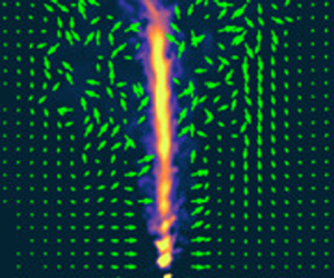
Figure 5 shows the particle image velocimetry (PIV) computed vertical and horizontal velocity fields from three L-experiments. In these experiments the background rotation is clockwise as seen from above ($\varOmega <0$). Because the plume was not dyed in the L-experiments, the location of the plume in the vertical (top row) and horizontal (middle row) is instead visualized by a grey scale showing the measured speed of the flow. Arrows indicate the motion of the surrounding ambient fluid.

Figure 5. Velocities measured using PIV in three L-experiments showing (a) no tornado formation in weak background rotation and moderate volume flux (left column), (b) tornado formation in moderate background rotation and moderate volume flux (Expt L10, middle column) and (c) no tornado formation in moderate background rotation and large volume flux (right column). In all experiments $H_0=21\ \textrm {cm}$ and $\rho _0=1.066\ \mbox {g}\ {\mbox {cm}}^{-3}$. The top row shows velocity (green arrows) and speed (grey scale) from vertical cross-sections at $t=25\ \textrm {s}$ after the start of an experiment. The velocity magnitude and speed for all three panels are indicated at the bottom of the top-middle plot. Arrows are plotted only if their magnitude is less than $0.6\ \mbox {cm}\ \mbox {s}^{-1}$. Likewise, the middle row shows velocity and speed from horizontal cross-sections 6 cm below the source at $t=25\ \textrm {s}$. These plots are shifted so that the velocity is plotted about the centroid of the speed at $(x_c,y_c)$. The bottom row shows radial time series of the azimuthal velocity which is azimuthally averaged about the centroid. For $0\leqslant r\lesssim 1\ \textrm {cm}$, zero values are assigned to data where the standard deviation of the azimuthal average exceeds the mean value.

In the experiment with relatively low rotation (figure 5a), the plume at $t=25\ \textrm {s}$ was in the process of being deflected from the vertical axis with strong vertical and radial motions being evident near the source. At a distance 6 cm from the source, the cyclonic (clockwise) horizontal flow around the plume remained approximately axisymmetric, although the radial time series of the azimuthal flow (bottom row) shows that its radial extent broadened substantially after the plume was deflected off axis shortly after 25 s. In contrast, in the experiment with the same source volume flux but three times the background rotation, the plume transformed into a tornado after 17 s. The maintenance for up to 60 s of large azimuthal vorticity associated with the tornado is evident in the radial time series of $u_\theta$ (figure 5b, bottom): after 25 s the radial extent of the peak in $u_\theta$ remains approximately constant while the peak value increases moderately in time. Despite the coherent structure of the vortex, strong radial and vertical circulations are evident in the vertical cross-section at $t=25\ \textrm {s}$. Eventually these motions resulted in the breakdown of the tornado. In the experiment with the same background rotation as that in figure 5(b), but with double the source vertical velocity, the plume became significantly deflected from the vertical axis at $t=25\ \textrm {s}$. While the ambient motion in the vertical plane appeared to be turbulent, there remained a coherent azimuthal flow around the centroid of the plume, although the radial time series (figure 5c, bottom) shows the flow was relatively weak and broadened radially over time.

3.3. Parameter regime for tornado formation

In experiments for which a tornado occurred, analyses were performed, with results given in table 1. It was often observed that the fluid from the source was deflected off axis shortly before the formation of the tornado and that when the tornado did form, its axis was displaced from the $z$-axis overlying the source. The time, $T_t$, when the tornado first began to develop near the source was determined somewhat subjectively by watching movies of the experiments, and identifying when the flow leaving the nozzle became columnar in structure. Generally, $T_t$ was found to be longer in experiments with slower rotation. Although there was some variation, in part due to the somewhat subjective assessment of $T_t$, typically we found that the tornado-formation time was approximately a half-period of background rotation: $T_t\sim 3/\varOmega$.

The radial displacement from the $z$-axis, $r_c=|\boldsymbol {x}_c|$, of the tornado as a function of vertical distance from the source was measured by locating the centroid of the speed measured by horizontal PIV. This value was averaged over times between $5$ and 10 s after the unambiguous formation of the tornado. Typical displacements were found to be of the order $r_c\simeq 1\ \textrm {cm} = 5b_0$. Once formed, however, the tornado exhibited little horizontal variation in its location. The strength of the tornado was assessed by the maximum azimuthally averaged azimuthal velocity, $U_{\theta t}$. In some experiments, particularly those with small $r_c$, the strength increased approximately linearly in time for tens of seconds. In experiments that ran for long times, a tornado typically persisted for about a minute before collapsing to form a turbulent plume deflected from the vertical axis. Tornados that formed at distances larger than $r_c=1\ \textrm {cm}$ from the $z$-axis typically had smaller maximum azimuthal velocity, $U_{\theta t}$ and larger radius, $b_{\theta t}$, where this maximum was attained. (Here and elsewhere the ‘$t$’ subscript refers to measurements of the tornado.)

Although these diagnostics provide some qualitative insight into the properties of the tornados, they are limited by the measurements which were too noisy near the tornado core to extract reliable information about the radial structure of the azimuthal velocity. As shown in numerical simulations below, the actual radius, $b_{\theta t}$, of the tornado was closer to that of the nozzle radius, and the radial displacement of the tornado axis from the $z$-axis above the source was less than $3b_0$.

Although identical experiments could be run with a tornado appearing in one and not in the other, there appeared to be a ‘sweet spot’ of parameters for which a tornado was more likely to occur. Figure 6 shows regime diagrams indicating parameters resulting in tornado formation in at least one experiment (circles) or not at all (crosses). Both for moderate plume density (figure 6a) and high plume density (figure 6b), it appeared as though a tornado was less likely to occur if the source vertical velocity or background rotation was too large. Of course, no tornado occurred if there was no background rotation. The reason for the increased likelihood of tornado for certain parameters is elucidated through the analysis of numerical simulations and discussion that follow.

Figure 6. Regime diagrams showing parameters for which a tornado was well established for long time (circles), began to form before being disrupted within 5 s (squares) and for which a tornado never formed even in repeat experiments (crosses), as observed in L-experiments with source density (a) $\rho _0=1.066\ \mbox {g}\ {\mbox {cm}}^{-3}$ and (b) $\rho _0=1.13\ \mbox {g}\ {\mbox {cm}}^{-3}$. The dashed lines indicate values of $w_0$ for which ${\mathcal {B}}_0=1$.

4.1. Qualitative results for three simulations

We begin with an overview of three simulations with rotation rate, source velocity and source reduced gravity identical to the experiments presented in figure 5 except that in the simulations the background rotation is counterclockwise ($\varOmega >0$) and the source is positively buoyant originating from the bottom. As in the experiments with no tornado formation evident (figure 5a,c), the simulations resulted in the plume eventually being deflected off axis and remaining turbulent if $\varOmega =0.1\ {{\mbox {s}}^{-1}}$ and $w_0=5.7\ \mbox {cm}\ \mbox {s}^{-1}$ (S1), and if $\varOmega =0.3\ {{\mbox {s}}^{-1}}$ and $w_0=11.4\ \mbox {cm}\ \mbox {s}^{-1}$ (S10). A tornado formed in the simulation with $\varOmega =0.3\ {{\mbox {s}}^{-1}}$ and $w_0=5.7\ \mbox {cm}\ \mbox {s}^{-1}$ (S7). For each simulation, figure 7 shows vertical cross-sections through the plume of the in-plane velocity and density perturbation (top row of plots), and it shows horizontal cross-sections of horizontal velocity and vertical vorticity (bottom row of plots). While the full vertical extent of the domain is shown in the top plots, only half the lateral extent is shown in all the plots.

Figure 7. Corresponding to the experiments shown in figure 5, snapshots at $t=25\ \textrm {s}$ from simulations (a) S1, (b) S7 and (c) S10 having $|g_0^{\prime }|=65\,\mbox {cm}\ {\mbox {s}}^{-2}$ and rotation and source velocity as indicated in the top row of plots: (top row) in-plane velocity $(v,w)$ (arrows) and perturbation density (colour) in the $(y,z)$-plane; (bottom row) horizontal velocity (arrows) and vertical component of vorticity, $\zeta$, (colour) in a horizontal plane at $z=2$ cm (a height chosen to be close to the effective virtual origin for lazy plumes). In all cases, arrows are shown only if their magnitude is less than $1\ \mbox {cm}\ \mbox {s}^{-1}$. The scale of the arrows in all plots is indicated above the bottom-left plot.

In simulation S1 (figure 7a), which had source Rossby number ${\textit {Ro}}_0=143$, the structure of the plume at $t=25\ \textrm {s}$ ($0.4$ of a rotational period) was qualitatively similar to that in a non-rotating fluid: the plume remained centred about the vertical axis and widened as the buoyancy decreased with height due to ambient fluid entrainment. Except near the turbulent eddies in the plume and near the top of the domain, the ambient motion was predominantly horizontal with a cyclonic (counterclockwise) circulation around the plume (figure 7a, bottom) as a consequence of entrainment drawing the rotating ambient fluid radially inward. In this simulation, the plume was found to deflect from the vertical axis at $T_d=28\ \textrm {s}$.

In stark contrast, simulation S7 (figure 7b) shows that the plume transformed into a tornado, doing so at time $T_t\simeq 17\ \textrm {s}$. This simulation was run with the same parameters as experiment L10 (figure 5b). In that experiment a tornado also formed, but around 20 s. The simulated tornado was characterized by a tight, vertically extended core of fluid whose density changed little with height up to $z\simeq 15\ \textrm {cm}$. The vertical cross-section shows that the ambient velocity is primarily horizontal up to $z\simeq 5\ \textrm {cm}$ from the source at $t=25\ \textrm {s}$, with an apparent rightward velocity component over the bottom ${\simeq }5\ \textrm {cm}$ to either side of the tornado. This occurs in part because some entrainment continues to take place, but also because the centre of the vortex is displaced in the negative $x$-direction from the $z$-axis above the source (see figure 7b, bottom) so that the flow in the $x=0$ plane captures some of the anticyclonic azimuthal flow going around the tornado. Despite the presence of moderate rotation, there are significant vertical as well as horizontal motions in the ambient fluid well outside the tornado above $z\simeq 5\ \textrm {cm}$. The horizontal cross-section (figure 7b, bottom) shows strong cyclonic motion surrounding a localized core of positive vertical vorticity having a radius $b_{\theta t}\simeq 0.3\ \textrm {cm}$. The maximum vorticity is $67\ {{\mbox {s}}^{-1}} = 112 f$. We further note the occurrence of quasi-periodic perturbations to the columnar vortex between $z\simeq 1$ and $6\ \textrm {cm}$ (figure 7b, top). These may be a consequence of inertial waves trapped within the vortex, as has been observed in experiments of decaying rotating turbulence generated by oscillating grids (Hopfinger, Browand & Gagne Reference Hopfinger, Browand and Gagne1982; Davidson, Staplehurst & Dalziel Reference Davidson, Staplehurst and Dalziel2006; Staplehurst, Davidson & Dalziel Reference Staplehurst, Davidson and Dalziel2008). However, a detailed examination of these disturbances lies beyond the focus of our study.

In the simulation with the same background rotation but with twice the vertical velocity at the source (S10), the plume first deflected significantly off-axis at $T_d=14\ \textrm {s}$ and remained deflected at $t=25\ \textrm {s}$, as shown in figure 7(c). Although the ambient flow outside the plume is primarily horizontal below $z\simeq 5\ \textrm {cm}$, the $y$-velocity is positive on either side of the plume as a consequence of the centroid of the disturbance being shifted to the second quadrant. The vertical vorticity at $z=2\ \textrm {cm}$ is no longer coherent and single-signed, although a near-axisymmetric azimuthal flow surrounds the centroid of the plume.

4.2. Time series analyses of the plume evolution

In order to gain insight into the dynamics governing the plume and ambient fluid evolution, vertical time series were constructed of the density normalized dynamic pressure, $P_c$, and vertical velocity, $W_c$, at the centroid of the flow, and of the maximum azimuthally averaged azimuthal velocity, $U_\theta$, about the centroid. The centroid itself, which can change position with height and time, was determined from the magnitude of the vertical vorticity field associated with the flow. After constructing the time series, MatLab's ‘rlowess’ method was used to smooth the data by averaging over 1 s in time and 1 cm in the vertical. This procedure helped to filter out fast- and fine-scale motions so as to focus on the statistically quasi-steady evolution of the fields. The results, corresponding to the three simulations in figure 7, are shown in figure 8. These fields are normalized using the effective source velocity, $w_{0,{eff}}$, defined by (2.8).

Figure 8. Vertical time series corresponding to the three simulations shown in figure 7 (S1 left, S7 middle, S10 right), showing fields evaluated about the plume centroid at $(x_c(z,t),y_c(z,t))$: (a–c) dynamic pressure, (d–f) vertical velocity, (g–i) maximum azimuthally averaged azimuthal velocity and (j–l) the plume Rossby number as given by (2.17). In the plots of $P_c/w_{0,{eff}}^2$, dashed lines indicate where the pressure is half its minimum value at $t=1\ \textrm {s}$. In the plots of $W_c/w_{0,{eff}}$, dashed lines indicate where the vertical velocity is half its maximum value at $t=1\ \textrm {s}$. In all plots, the crosses on the time axes represent the time, $T_d$, when the plume first deflected off axis. In the middle column of plots, the circle on the time axis indicates the time, $T_t$, when tornado formation was first evident. The arrow below the time series in (k) indicates the enhanced reduction in the Rossby number close to the source at early times compared with its value around the virtual origin at $z\simeq 2\ \textrm {cm}$. Note that the range of time in the first column of plots is twice that of the second and third columns.

The vertical time series of $P_c$ show the front of the starting plume rising past $z=15\ \textrm {cm}$ in the first two or three seconds of the simulation. The rise time depended upon the source buoyancy. (Note that the apparently steeper slope of the front of the starting plume in figure 8(a,d,g,j) is due to the time axis extending to 40 s, rather than 20 s in figure 8(b,c)). The pressure decreased rapidly in the vertical from the source to $z\simeq 2\ \textrm {cm}$, close to the location of the lazy plume virtual origin. It is over this distance that the relatively low momentum of the lazy plume adjusts to become closer to that of a pure plume. Above the virtual origin the pressure increased with height corresponding to the decrease in the vertical velocity, as expected for a pure plume. The right and upward streaks in the pressure time series correspond to unfiltered turbulent eddies rising upward through the ascending plume. Unlike a plume with no background rotation, as time progressed the vertical extent of the low-pressure region above the virtual origin became smaller as is evident, for example, in figure 8(b) by the converging dashed lines indicating where the pressure is half the minimum pressure at $t=1\ \textrm {s}$. The vertical extent of the low-pressure region decreased more rapidly in simulations S7 and S10, which had faster background rotation (figure 8b,c). The corresponding increasing dominance of an adverse vertical pressure gradient approaching the source in time was likewise noted in the simulations of rotating plumes in (non-uniformly) stratified fluid by Fabregat Tomàs et al. (Reference Fabregat Tomàs, Poje, Özgökmen and Dewar2016).

The low-pressure region vanished altogether at the critical time $T_d\simeq 28\ \textrm {s}$ in simulation S1 (figure 8a), at $T_d\simeq 14\ \textrm {s}$ in simulation S7 (figure 8b) and at $T_d\simeq 13\ \textrm {s}$ in simulation S10 (figure 8c). At these times the plumes deflected from the vertical axis at the source. After these times, in the first and last cases the pressure became somewhat homogeneous with height, corresponding to the source fluid being deflected significantly away from the vertical. In the middle case (figure 8b), shortly after the low-pressure region vanished the pressure near the source decreased rapidly once more and the vertical extent of the low-pressure region then extended well above the source after time $T_t\simeq 18\ \textrm {s}$ corresponding to the formation of a tornado having azimuthal velocity in cyclostrophic balance with the radial pressure gradient.

The descent toward the source over time of relatively higher pressure coincided with a decrease in the vertical velocity within the plume (figure 8d–f). In particular, the positive vertical strain near the source vanished at the deflection time $T_d$, at which time the vertical velocity near the virtual origin was approximately $0.5w_{0,{eff}}$. This dynamics lies in stark contrast with non-rotating plume theory. Not only was the evolution of the rotating plume unsteady, but the system evolved from one having decreasing vertical velocity with height above the virtual origin to one in which the vertical velocity was near uniform with height at the time when the pressure low vanished.

The change in the centreline pressure and vertical velocity can be attributed to the increase of azimuthal velocity in the plume, as shown by the time series of $U_\theta$ in figure 8(g–i). Entrainment of the rotating ambient fluid surrounding the plume efficiently increased the azimuthal velocity within the plume by way of angular momentum conservation. As $U_\theta$ increased, a greater vertical strain was required in order to change both the radial and azimuthal velocities. If the buoyant flow possessed insufficient potential energy to supply the requisite kinetic energy, then vertical motion became inhibited.

As a measure of the importance of azimuthal flows in influencing the plume dynamics, figure 8(j–l) shows time series of the plume Rossby number, $\textit {Ro}_{{p}}$, defined by (2.17). Associated with the growth of $U_\theta$ in the plume is the increase in characteristic vertical vorticity $\zeta_{\theta} \equiv 2U_\theta /b_\theta$. Even though at early times the vertical velocity was much larger than $U_\theta$, $\zeta_{\theta}$ quickly became much larger than $f$, so that $\textit {Ro}_{{p}}\simeq W_c/U_\theta = 1/q$ rapidly reduced. This reduction occurred most rapidly well above the source because ambient fluid was carried radially inward over a larger distance, owing to the larger plume radius. This resulted in a larger spin-up due to angular momentum conservation.

Also evident in our simulations of lazy plumes was a more rapid decrease in the plume Rossby number close to the source as compared with the change in the plume Rossby number moderately above the height of the virtual origin (around $z\simeq 2\ \textrm {cm}$). This was particularly evident in simulation S7 (indicated by the arrow below figure 8k), which had higher source buoyancy parameter (${\mathcal {B}}_0=5.0$) than that in simulation S10 with the same background rotation (${\mathcal {B}}_0=1.3$).

4.3. Time series analyses of the ambient flow surrounding plume

The evolution of the ambient fluid motion around the plume is examined by constructing vertical time series of the radial, azimuthal and vertical velocities that are azimuthally averaged around a radius $r_a=3\ \textrm {cm}$ from the centroid of the flow. This radius was chosen to be close to the boundary at $z=15\ \textrm {cm}$ between the turbulent plume and ambient fluid at early times in the simulations. The resulting time series are shown in figure 9 for the same three simulations with snapshots shown in figure 7.

Figure 9. Vertical time series corresponding to the three simulations shown in figure 7 (S1 left, S7 middle, S10 right), showing azimuthally averaged normalized velocities at $r_a=3\ \textrm {cm}$: (a–c) radial velocity, (d–f) azimuthal velocity and (g–i) vertical velocity. In the plots of $u_r/w_{0,{eff}}$, the thick contour indicates where the radial velocity is zero and solid and dashed contours are plotted at intervals of $0.01$. In the plots of $u_\theta /w_{0,{eff}}$, black contours are plotted at intervals of $0.2$; the thick contours indicate where the azimuthal velocity is zero. The yellow contours in this plot indicate where the ambient Rossby number is $0.1$ (thick line) and $0.5$ (thin line). In the plots of $w/w_{0,{eff}}$, contours are plotted at $-0.01$ (dashed), $0$ (thick solid) and $0.01$ (solid). Note that the range of time in the first column of plots is twice that of the second and third columns.

As the front of the starting plume rose, the ambient fluid was first pushed radially outward around its head, but the flow then reversed to be drawn into the plume itself. The inward radial flow was generally faster further above the source and fluctuated as successive eddies rose upward through the plume. Of course, theory predicts the radial entrainment velocity ($\propto W_c$) is smaller with increasing height above the virtual origin. However, as given by (2.18), at a fixed radius outside the plume the radial inflow is larger with height.

In all simulations, the radial and azimuthal velocities initially exhibited vertical shear. However, approaching the time, $T_d$, at which the plume was deflected from the vertical, azimuthal velocity contours became nearly vertical for $z\gtrsim 0$. Contours of the ambient Rossby number, $\textit {Ro}_{{a}}$ (defined by (2.19)), are superimposed on the vertical time series of $u_\theta$ (figure 9d–f). If $u_r$ was neglected in the definition of $\textit {Ro}_{{a}}$, the contours would coincide with lines of constant $u_\theta$. It is clear that well above the source ($z\gtrsim 5\ \textrm {cm}$) at early times the radial velocity contributes significantly to increase the ambient Rossby number beyond $0.1$ (thick yellow contour in figure 9d–f). Close to the source, the Rossby number remained smaller for longer times leading to the vertical shear being reduced more rapidly there.

These considerations lead to a complicated evolution of the ambient vertical velocity field (figure 9g–i). As the front of the starting plume passed a given height it induced a downward velocity in the surrounding ambient. Thereafter, below $z\simeq 5\ \textrm {cm}$ a net upward flow developed, increasing upward from zero at $z=0$, reaching a maximum and then decreasing again. The corresponding vertical strain near $z=0$ acted to reduce the vertical shear of $u_r$ and $u_\theta$.

4.4. Temporal evolution of flow near the source before plume deflection

Corresponding to the three simulations examined above, figure 10(a–c) plots the radial dependence at $z=2\ \textrm {cm}$ (close to the lazy plume virtual origin) and $t=10\ \textrm {s}$ of the most significant forcing terms in the radial and azimuthal momentum equations (2.11) and (2.12). Specifically, these are the radial pressure gradient ($\partial P/\partial r$), the Coriolis accelerations ($\kern0.06em f u_\theta$ and $-f u_r$) and the centripetal acceleration ($u_\theta ^2/r$). For simulation S1 ($\varOmega =0.1\ {{\mbox {s}}^{-1}}$), the radial pressure gradient dominated over the Coriolis and centripetal accelerations at $t=10\ \textrm {s}$ ($0.16$ of a rotational period) so that the inward radial flow increased in time. Conversely, in the simulations with $\varOmega =0.3\ {{\mbox {s}}^{-1}}$, the acceleration due to the radial pressure gradient was in near balance with the Coriolis acceleration ($\textit {Ro}_{{a}}\ll 1$) for $r\gtrsim 3\ \textrm {cm}$, and with the centripetal acceleration ($\textit {Ro}_{{a}}\gg 1$) for $r\lesssim 1\ \textrm {cm}$. Due to the vertical strain in the ambient fluid, the azimuthally averaged radial velocity field did not decay with radius as $r^{-1}$, as would be required by (2.10) with $\partial w/\partial z=0$. Instead, it decayed as

(4.1)\begin{equation} u_r \propto r^{{-}p_r}, \end{equation}

with $p_r\simeq 0.33$ in simulation S1 and $p_r\simeq 0.5$ in simulations S7 and S10. The radial profile of azimuthal velocity also exhibited power law behaviour near the plume according to

(4.2)\begin{equation} u_\theta \propto r^{{-}p_\theta}, \end{equation}

although $p_\theta$ was typically larger than $p_r$. The power law exponents for all simulations are given in table 2. Generally $p_r<1$ and $p_\theta <1$ except in the simulation of a jet (S4) and the simulations with the fastest rotation (S11 and S12), for which $p_r\simeq 1$.

Figure 10. For the three simulations shown in figure 7, analyses showing the following: (a–c) log–log plots of the azimuthally averaged radial profiles at $t=10\ \textrm {s}$ and $z=2\ \textrm {cm}$ of the density normalized pressure gradient (thick blue), centripetal acceleration (dashed), the Coriolis acceleration in the radial momentum equation (solid black) and the Coriolis acceleration in the azimuthal momentum equation (solid red); (d–f) time evolution at $r_a=3\ \textrm {cm}$ and at three different heights (as indicated in (d)) of the normalized azimuthally averaged radial and azimuthal velocities; (g–i) time evolution within the plume at $z=2\ \textrm {cm}$ of normalized maximum vertical vorticity ($\zeta _\theta \equiv 2U_\theta /b_\theta$, black), maximum vertical velocity (red) and the maximum azimuthally averaged azimuthal velocity (green). In the top row dotted lines are the offset best-fit lines to $fu_\theta$ (black) and $fu_r$ (red) with numbers indicating the slope and associated error. In the middle row the red dotted lines show the offset best-fit line to $u_r(t;z=2\ \mbox {cm},r=3\ \mbox {cm})/w_{0,{eff}}$ over the time range indicated, with numbers giving the slope. In (d–i), the crosses and circles on the time axes respectively indicate when the plume first deflected and when it first transformed into a tornado.

This analysis was also performed by extracting at $t=10\ \textrm {s}$ radial profiles taken at $z=1$ and $z=3\ \textrm {cm}$ (not shown). The results showed that the computed power law exponents, $p_r$ and $p_\theta$, did not vary significantly with height for $z=2\ (\pm 1)\ \textrm {cm}$. However, the magnitude of the radial and azimuthal flows did increase in time. The time evolution of the azimuthally averaged ambient flow at $r=r_a=3$ and $z=2\ \textrm {cm}$ is plotted in figure 10(d–f) for the three simulations considered above. These show that the inward radial flow increases linearly in time according to

(4.3)\begin{equation} u_r(r_a=3\ \mbox{cm},t)/w_{0,{eff}} \simeq{-}\dot{c}_r f t, \end{equation}

in which $\dot {c}_r$ is an empirically determined constant. In all simulations (see table 2), we find $\dot {c}_r \simeq 0.0020\pm 0.0005$. Because the Coriolis term, $-fu_r$, is the dominant driving force in the azimuthal momentum equation (2.12), the azimuthal velocity is expected to increase quadratically in time according to

(4.4)\begin{equation} u_\theta(r_a=3\ \mbox{cm},t)/w_{0,{eff}} \simeq \ddot{c}_{\theta} (f t)^2/2, \end{equation}

in which $\ddot {c}_{\theta }$ is an empirically determined constant. This constant is found to be comparable to $\dot {c}_r$, as expected (see table 2).

Combining these results, a crude representation of the evolution of the ambient flow around $z=2\ \textrm {cm}$ (near the virtual origin) is

(4.5a,b)\begin{equation} \frac{u_r(r,t)}{w_{0,{eff}}} \simeq{-}\dot{c}_r\ (ft) \left(\frac{r}{r_a}\right)^{{-}p_r}, \quad \frac{u_\theta(r,t)}{w_{0,{eff}}} \simeq \frac{1}{2}\ddot{c}_{\theta} (ft)^2 \left(\frac{r}{r_a}\right)^{{-}p_\theta}. \end{equation}

Figure 10(g–i) examines the time evolution of the centreline vertical vorticity, the maximum azimuthally averaged azimuthal velocity and its associated vorticity within the plume at $z=2\ \textrm {cm}$. This shows that $W_c$ remains constant even as $U_{\theta }$ increases until $q=U_{\theta }/W_c\simeq 0.15$, consistent with our prediction that rotation significantly influences the plume if the swirl exceeds the critical value $q_c\simeq 0.15$ (see § 2.2). Particularly for lazy plumes, until close to the time of plume deflection the maximum azimuthal velocity was found to increase approximately linearly in time according to

(4.6)\begin{equation} U_\theta/w_{0,{eff}} \simeq c_{\alpha} ft. \end{equation}

In most simulations, $c_{\alpha } = 0.03 (\pm 0.01)$. The largest value $c_{\alpha } \simeq 0.04$ was measured in the simulation with largest source buoyancy parameter (${\mathcal {B}}_0=9.9$) and the smallest value $c_{\alpha }\simeq 0.012$ was measured in the simulation of a jet (${\mathcal {B}}_0=0$). This suggests that the linear increase in time of $U_\theta$ within the plume, as opposed to the quadratic increase in the surrounding ambient, was strongly influenced by the reduction in entrainment into lazy plumes, with entrainment being further reduced as the surrounding fluid acquired greater azimuthal velocity. This assertion is supported by comparing (4.6) with (2.16), showing that the estimated entrainment coefficient, $\alpha _{{B}}\sim c_{\alpha }$, is approximately a third of the value expected for a pure plume. The positive vertical strain near the source of lazy plumes acted to increase the absolute vorticity both of the fluid that was entrained and of the fluid leaving the source. Plumes that were closer to being pure near the source had zero or negative vertical strain associated with the decrease in mean vertical velocity with height. So, while their relative entrainment of the surrounding azimuthal flow was larger, the associated vorticity within the plume was reduced.

4.5. Plume deflection

In all cases, the vertical velocity in the plume at $z=2\ \textrm {cm}$ began to decrease when $w_{0,{eff}}/(\zeta_{\theta} b_0) \sim 4$, which nearly coincides with the critical Rossby number, ${\textit {Ro}}_c=3.4$, at which rotation was found in experiments by Fernando et al. (Reference Fernando, Chen and Ayotte1998) to constrain vertical motion in a plume. The decrease is associated with the change in pressure within the plume due to the increasing surrounding azimuthal flow.

Near the plume the ambient flow is in near cyclostrophic balance so that the radial pressure gradient is approximately equal to the centripetal acceleration, $u_\theta ^2/r$ (figure 10b,c). Hence, the pressure surrounding the plume near the source decreases as a fourth power of time. Using (4.5a,b), a semi-empirical estimate of the pressure surrounding the plume around the virtual origin is given by

(4.7)\begin{equation} \frac{P}{{w_{0,{eff}}}^2} \sim{-}\frac{\ddot{c}_{\theta}^2}{8p_\theta} (ft)^4 \left(\frac{r}{r_a}\right)^{{-}2p_\theta}, \end{equation}

in which $r_a=3\ \textrm {cm}$ and, based on measurements of lazy plume simulations, we estimate $p_\theta \simeq 0.7$ and $\ddot {c}_{\theta }\simeq 0.003$. Around the time of a half-rotation period, for which $ft\simeq 6$, this expression evaluated at $r=b_0$ gives $P/{w_{0,{eff}}}^2 \simeq -0.05$, which is comparable to the pressure at the source. This suggests the plume deflection occurs not just due to the build-up of an adverse vertical pressure gradient but also because the ambient flow ultimately reverses the radial pressure gradient near the source on a time of the order $T_d\sim 6/f$.

4.6. Tornado structure and stability

In the four simulations for which a stable tornado formed, the flow and structure of the tornado were measured at a time 5 s after the tornado first began to develop such that it extended beyond 10 cm above the source. At each height the velocity fields were computed from an azimuthal average around the centroid of the vertical vorticity field associated with the flow, from which were extracted at each height the maximum vertical velocity, $W_{ct}$, the maximum azimuthal velocity, $U_{\theta t}$, and the width, $b_{\theta t}$, where the azimuthal velocity was largest. The resulting vertical profiles are plotted in figure 11.

Figure 11. Vertical profiles of normalized fields associated with a tornado in simulations for which a stable tornado appears showing (a) maximum azimuthal velocity, (b) radial extent, (c) centreline vertical velocity and (d) radial distance of the centroid from the $z$-axis. The parameters for each simulation, with values in cgs units, are indicated in (a).

In all four cases $U_{\theta t}$ moderately decreased with height between $1$ and $10$ cm above the source and, consistent with the suppression of three dimensional turbulent motions, $U_{\theta t}$ was smaller than $w_{0,{eff}}$, the effective source vertical velocity. The radial extent of the tornado, $b_{\theta t}$, was approximately twice the source radius, $b_0$, showing an increase with height that was much smaller than that associated with a turbulent plume.

The maximum vertical velocity generally increased with height at least up to $z=5\ \textrm {cm}$, consistent with the vortex being stretched. Between the four simulations with a tornado there was significant variation in typical values of $W_{ct}$ (figure 11c). This can be explained by the plot in figure 11(d) showing the radial distance, $r_c$, of the centroid of the tornado from the $z$-axis as a function of height. In simulations where the tornado was most closely aligned above the source such that $r_c\simeq b_0$, the maximum azimuthal and vertical velocities were largest and the radius of the tornado was smallest. However, in simulations where the fluid from the source was deflected by a significant radial distance before the tornado formed ($r_c\simeq 2b_0$), the radius was larger and the velocities smaller. A similar observation was made for tornados that formed in laboratory experiments.

The stability of the tornado is assessed through examining its associated swirl. In studies of the stability of a columnar Gaussian (Batchelor) vortex having both azimuthal and axial flow (Batchelor Reference Batchelor1964; Delbende, Rossi & Le Dizès Reference Delbende, Rossi and Le Dizès2002) the swirl is defined by $q_t^\star \equiv \varGamma /(2{\rm \pi} b_t W_{ct})$, in which $b_t$ is the radius of the tornado, $W_{ct}$ is the centreline vertical velocity and $\varGamma$ is the (constant) circulation outside the tornado. Numerous theoretical studies of the temporal and absolute/convective instability of the Batchelor vortex with and without viscous effects have shown that the vortex is stable if $q_t^\star \gtrsim 1.5$ (e.g. see Lessen & Paillet Reference Lessen and Paillet1974; Lessen, Singh & Paillet Reference Lessen, Singh and Paillet1974; Stewartson & Leibovich Reference Stewartson and Leibovich1987; Delbende, Chomaz & Huerre Reference Delbende, Chomaz and Huerre1998).

It is more convenient for us to measure the maximum azimuthal velocity which, for a Batchelor vortex, is related to the circulation by $U_{\theta t} \simeq 0.639 \varGamma /(2{\rm \pi} b_t)$ (Lessen et al. Reference Lessen, Singh and Paillet1974). Therefore we define the swirl of a tornado by

(4.8)\begin{equation} q_t \equiv U_{\theta t}/W_{ct} \simeq 0.639 q_t^\star. \end{equation}

The corresponding condition for stability is given by $q_t\gtrsim 1$. Consistent with this prediction, the vertical profiles of $q_t$, plotted in figure 12, show that the swirl for all tornados was greater than $1$, at least below $z=5\ \textrm {cm}$. This analysis suggests that for a tornado to form after being deflected, the vorticity within the plume must increase sufficiently through vortex stretching so that the maximum azimuthal flow exceeds the axial flow.

Figure 12. Vertical profiles of the swirl associated with the tornados observed in four simulations. The line colours correspond to those shown in figure 11(a).