


1. Introduction
Nanofluidic transport involves the flow of liquids and flow-driven transport of ions, solutes, bioanalytes and other species in nanochannels and nanopores (Eijkel & Van Den Berg Reference Eijkel and Van Den Berg2005; Sparreboom et al. Reference Sparreboom, van den Berg and Eijkel2009; Das et al. Reference Das, Dubsky, van den Berg and Eijkel2012; Ziemys et al. Reference Ziemys, Kojic, Milosevic and Ferrari2012; Koltonow & Huang Reference Koltonow and Huang2016; Gao et al. Reference Gao, Feng, Guo and Jiang2017; Zhu et al. Reference Zhu, Wang, Tian and Jiang2019). Such transport has received immense attention over the past few decades motivated by its applications in fabricating sensors that require very little sample volumes (Venkatesan & Bashir Reference Venkatesan and Bashir2011; Miles et al. Reference Miles, Ivanov, Wilson, Doan, Japrung and Edel2013), devices capable of ionic gating (Liu et al. Reference Liu, Zhang, Li, Heng, Wang, Tian and Jiang2015; Fang et al. Reference Fang, Zhang, Yang, Wang, Tian, Zhang and Jiang2016), and platforms capable of a variety of biomedical applications (Hood et al. Reference Hood, Hood, Ferrari and Grattoni2017; Weerakoon-Ratnayake et al. Reference Weerakoon-Ratnayake, O'Neil, Uba and Soper2017), water filtration and desalination (Chen et al. Reference Chen2017; Anand et al. Reference Anand, Unnikrishnan, Mao, Lin and Huang2018), oil recovery (Zhang et al. Reference Zhang, Jia, Li and Liu2019), etc. The significantly large interfacial effects in such nanofluidic systems have enabled the utilization of novel and unconventional flow-driving mechanisms such as electro-osmotic (EOS) transport (Eijkel & Van Den Berg Reference Eijkel and Van Den Berg2005). The EOS flows are characterized by the water transport caused by the imposed axial electric-field-driven transport of the net charge imbalance of the electric double layer (EDL) created at the charged walls of the nanochannel. Such EOS transport in nanochannels can also be ‘induced’ by other mechanisms that trigger a migration of the charge imbalance of the EDL. Some of these mechanisms are the presence of an applied axial pressure gradient (this leads to the generation of a streaming electric field and a velocity field that is a combination of this pressure-driven flow field and an induced EOS flow field) (Chakraborty & Das Reference Chakraborty and Das2008; Das & Chakraborty Reference Das and Chakraborty2009, Reference Das and Chakraborty2010), an applied axial concentration gradient of solutes and/or ions (leading to a diffusio-osmotic (DOS) transport) (Qian, Das & Luo Reference Qian, Das and Luo2007; Jing & Das Reference Jing and Das2018), and an applied axial temperature gradient (leading to a thermo-osmotic (TOS) transport) (Dietzel & Hardt Reference Dietzel and Hardt2016, Reference Dietzel and Hardt2017).
The present paper probes the TOS transport in a nanochannel grafted with charged polyelectrolyte (PE) brushes in the presence of an imposed axial temperature gradient ( $\textrm {d}T/{\textrm {d} x}$). The presence of such a gradient along a charged nanochannel induces a pressure gradient and an electric field. The formation of an EDL at the nanochannel walls leads to the development of an osmotic pressure that depends on temperature (
 $T$), the number density of ions (
 $n_\infty$) and the EDL electrostatic potential (
 $\psi$). Therefore, the imposed axial gradient in temperature triggers a gradient in the (osmotic) pressure which is dictated by gradients in
  $T, n_\infty$ and
  $\psi$. The induced electric field, on the other hand, is contributed by all the factors that induce a differential migration of the cations and anions. There are three factors that contribute to this electric field: the conduction component, the thermal component and the osmotic component. The conduction component is dictated by the temperature gradient induced concentration gradient: this is an effect that is well-known as the Soret effect and it also depends on the ionic imbalance within the nanochannel EDL. The thermal component, on the other hand, is associated with the different thermophoretic mobilities of the ions. Finally, the osmotic component is associated with the flow-driven downstream advection of the charge imbalance present within the EDL. The TOS transport, therefore, is completely defined through the quantification of the induced electric field and the net flow field. This TOS fluid flow results from the flow associated with the induced pressure gradient (we can either call it a thermochemiosmotic flow, or split it further into a chemiosmotic (COS) flow and a thermal flow) and the flow associated with the induced electric field (i.e. the induced EOS flow). Over the past several years, such TOS transport in nanofluidic systems has been extensively studied (Dietzel & Hardt Reference Dietzel and Hardt2016, Reference Dietzel and Hardt2017) and has been identified to be useful in applications ranging from generating electricity in nanocellulose channels using waste heat (Li et al. Reference Li2019), energy conversion and storage (Chen et al. Reference Chen, Yao, Yan, Liu, Yang and Su2019), enhanced nanofluidic transport in presence of functionalization with PE brushes (Maheedhara et al. Reference Maheedhara, Jing, Sachar and Das2018a), etc. For the past decade and a half, functionalizing nanochannels with PE brushes has been employed for applications such as analyte and biomolecule sensing (Ali et al. Reference Ali, Tahir, Siwy, Neumann, Tremel and Ensinger2011), fabrication of ionic nanofluidic diodes and current rectifiers (Ali et al. Reference Ali, Ramirez, Mafe, Neumann and Ensinger2009, Reference Ali, Nasir, Ramirez, Cervera, Mafe and Ensinger2013; Yameen et al. Reference Yameen, Ali, Neumann, Ensinger, Knoll and Azzaroni2009, Reference Yameen, Ali, Neumann, Ensinger, Knoll and Azzaroni2010; Lin et al. Reference Lin, Lin, Hsu and Tseng2016), etc. Most of these applications rely on the strong environmental stimuli responsiveness of the PE brushes, which in turn significantly affects the ionic transport in such brush-functionalized nanochannels. The fluid flow is often significantly retarded in such brush-functionalized nanochannels stemming from the large drag forces exerted on the flow by the brushes (Chen & Das Reference Chen and Das2015a). Such reduced fluid flows are considered as a critical advantage of such brush-functionalized nanochannel systems: weak flow strength ensures that the differences in the ionic migration of the different ions, which is the key to several of the above applications, does not get masked by the background advective transport that acts equally on all the different types of ions. Very recently, in a series of papers (Chen & Das Reference Chen and Das2017Reference Chen and DasReference Zhulina, Pryamitsyn and Borisov; Chen, Sachar & Das Reference Chen, Sachar and Das2018; Maheedhara et al. Reference Maheedhara, Jing, Sachar and Das2018a,Reference Maheedhara, Sachar, Jing and Dasb; Sachar, Sivasankar & Das Reference Sachar, Sivasankar and Das2019a; Sivasankar et al. Reference Sivasankar, Etha, Sachar and Das2020a,Reference Sivasankar, Etha, Sachar and Dasb), however, we have established that such brush-induced weakening of flow strength in PE-brush-grafted nanochannels might not always be true. We showed that for certain cases where nanochannels are grafted with end-charged PE brushes (Chen & Das Reference Chen and Das2017; Chen et al. Reference Chen, Sachar and Das2018; Maheedhara et al. Reference Maheedhara, Jing, Sachar and Das2018a,Reference Maheedhara, Sachar, Jing and Dasb), some particular combination of grafting density, brush properties and salt concentration will lead to significantly enhanced nanofluidic EOS or induced EOS transport. We argued that such enhancement stemmed from the localization of the EDL charge density (and hence the EOS body force) away from the nanochannel wall (or the location of the maximum drag force). We have further established such localization of EOS-body-force-induced enhanced EOS or induced EOS transport in nanochannels grafted with backbone-charged PE brushes (Sachar et al. Reference Sachar, Sivasankar and Das2019a; Sivasankar et al. Reference Sivasankar, Etha, Sachar and Das2020a,Reference Sivasankar, Etha, Sachar and Dasb). Another possible factor, which was not identified in these papers and might have led to such an enhancement in the EOS or induced EOS transport in nanochannels grafted with end-charged or backbone-charged PE brushes (i.e. the setting that shifted the EDL charge density away from the nanochannel wall), was the possible molecular slip experienced by the liquid along the brush surface. We also compared the results between the cases of EOS and diffusio-osmotic transport in nanochannels grafted with end-charged and backbone-charged brushes. Our comparison revealed that the flow was more augmented for the case of nanochannels grafted with backbone-charged brushes stemming from a more appropriate prediction of the brush-induced drag force on the flow for such cases (Sivasankar et al. Reference Sivasankar, Etha, Sachar and Das2020a,Reference Sivasankar, Etha, Sachar and Dasb). Following this approach, we also compared the findings from this present study to that of diffusio-osmotic transport (Sivasankar et al. Reference Sivasankar, Etha, Sachar and Das2020a) in nanochannels grafted with backbone-charged PE brushes (see appendix A). In this study, we explore the influence of the TOS effects, triggered by the application of an axial temperature gradient, in significantly enhancing the liquid transport in nanochannels grafted with backbone-charged, pH-responsive PE brushes. The PE brushes are modelled using our recently developed augmented strong stretching theory (SST) model (Sachar et al. Reference Sachar, Sivasankar and Das2019a, Reference Sachar, Sivasankar, Etha, Chen and Das2020; Sachar, Sivasankar & Das Reference Sachar, Sivasankar and Das2019b). Our model, by accounting for the excluded volume interactions between PE brush segments and a more expanded form of the mass action law, modified the existing SST model that has been well-known for capturing the thermodynamics, electrostatics and configurations of the strongly stretched PE brushes (Lyatskaya et al. Reference Lyatskaya, Leermakers, Fleer, Zhulina and Birshtein1995; Zhulina & Borisov Reference Zhulina and Borisov1997; Zhulina, Klein Wolterink & Borisov Reference Zhulina, Klein Wolterink and Borisov2000; Lebedeva, Zhulina & Borisov Reference Lebedeva, Zhulina and Borisov2017). We first quantify the thermo-osmotically induced electric field and point out the individual contributions of conduction, thermal and osmotic components. Each of these components has contributions from the salt ions as well as the
  $\textrm {H}^+$ and
  $\textrm {OH}^-$ ions (please see the online supplementary materials available at https://doi.org/10.1017/jfm.2021.281). Subsequently, we study the overall TOS liquid transport, characterized by the TOS flow velocity. To better understand the variation of the TOS velocity, we study the individual contributions of the COS component, thermal component and the EOS component. We observe that the thermal and the COS components are invariably in the same direction and the net direction of the flow is eventually dictated by the relative strength (with respect to the other components) and direction of the induced EOS transport (or the induced TOS electric field). We compare both the electric field and the velocity field results with those of the brushless nanochannels having the same overall charge density as the brush-grafted nanochannels. We clearly find that the overall TOS velocity is significantly enhanced for the case of the brush-grafted nanochannels. A key factor responsible for causing the enhancement in the TOS liquid transport in the brush-grafted nanochannels in comparison with that in brush-free nanochannels is the localization of the EDL (and hence the EOS body force) away from the nanochannel walls. Even in our previous papers, probing the EOS flow (Sivasankar et al. Reference Sivasankar, Etha, Sachar and Das2020b) or diffusio-osmotic flow (one kind of induced EOS flow) (Sivasankar et al. Reference Sivasankar, Etha, Sachar and Das2020a), we have identified and attributed such a flow enhancement in brush-grafted nanochannels (in comparison with the brush-free nanochannels with identical charge density) to this localization of the EDL (and hence the EOS body force) away from the nanochannel wall. To reiterate, we are comparing here two cases: a brush-free nanochannel and a brush-grafted nanochannel. The basis of comparison is that the charges on the walls of the brush-free nanochannel are considered to be distributed on the brushes (grafted on a charge-free wall) in brush-grafted nanochannels. Therefore, the presence of the brushes shifts the centre of the charges (and hence the EDL induced by these charges and the consequent EOS body force) away from the nanochannel wall. One can easily show that for a flow in a nanochannel driven by an external force, the net flow rate increases with an increase in the distance (from the nanochannel wall) at which this external force is localized and this increase becomes maximum if this force is localized at the nanochannel centre. The presence of the brushes causes this localization and hence aids flow enhancement. However, the same very presence of the brushes subjects the flow to an additional drag force. Therefore, the brushes trigger two competing mechanisms (in the context of the electrokinetic fluid flow): localization of the EOS body force that enhances the flow and the presence of the additional brush-induced drag that reduces the flow. For certain parameter combinations, the effect of the localization of the EOS body force overwhelms the effect of the brush-induced drag, thereby enhancing the net flow rate. This is the central idea of this paper. It is also very pertinent to point out here that a large number of studies from other research groups have probed such electrokinetic transport in nanochannels/nanopores grafted with PE brushes (Yeh et al. Reference Yeh, Zhang, Hu, Joo, Qian and Hsu2012a,Reference Yeh, Zhang, Joo, Qian and Hsub,Reference Yeh, Zhang, Qian, Hsu and Tsengc; Benson et al. Reference Benson, Yeh, Chou and Qian2013; Milne et al. Reference Milne, Yeh, Chou and Qian2014; Zeng, Ai & Qian Reference Zeng, Ai and Qian2014; Zeng et al. Reference Zeng, Yeh, Zhang and Qian2015; Poddar et al. Reference Poddar, Maity, Bandopadhyay and Chakraborty2016; Zhou et al. Reference Zhou, Mei, Su, Yeh, Zhang and Qian2016; Zimmermann et al. Reference Zimmermann, Gunkel-Grabole, Bünsow, Werner, Huck and Duval2017; Sadeghi Reference Sadeghi2018; Sin & Kim Reference Sin and Kim2018; Hsu et al. Reference Hsu, Yang, Lin and Tseng2019; Huang & Hsu Reference Huang and Hsu2019; Lin et al. Reference Lin, Hsu, Lin and Tseng2019; Reshadi & Saidi Reference Reshadi and Saidi2019; Sadeghi, Azari & Hardt Reference Sadeghi, Azari and Hardt2019; Khatibi, Ashrafizadeh & Sadeghi Reference Khatibi, Ashrafizadeh and Sadeghi2020; Sadeghi et al. Reference Sadeghi, Saidi, Moosavi and Kroger2020a,Reference Sadeghi, Saidi, Moosavi and Sadeghib; Silkina, Bag & Vinogradova Reference Silkina, Bag and Vinogradova2020; Talebi, Ashrafizadeh & Sadeghi Reference Talebi, Ashrafizadeh and Sadeghi2021; Wu & Hsu Reference Wu and Hsu2021). They use exactly the same form of equation (see the 1st equation of (2.17) later) as ours. This equation is a ‘Brinkman’-like equation and is also sometimes denoted as the Stokes–Brinkman equation (Yeh et al. Reference Yeh, Zhang, Hu, Joo, Qian and Hsu2012a,Reference Yeh, Zhang, Joo, Qian and Hsub,Reference Yeh, Zhang, Qian, Hsu and Tsengc; Zeng et al. Reference Zeng, Ai and Qian2014, Reference Zeng, Yeh, Zhang and Qian2015; Sadeghi Reference Sadeghi2018). It provides a gross representation of the contribution of the brushes by considering the PE brush layer to be represented as a porous medium. It considers that the brushes do two things: (1) they trigger a particular EDL distribution and hence a particular distribution of the EOS body force (and other possible forces related to the EDL) and (2) they impart an additional gross drag force (with drag coefficient varying quadratically with the monomer distribution) on the fluid flow. In this context, the natural question arises that why these other papers (Yeh et al. Reference Yeh, Zhang, Hu, Joo, Qian and Hsu2012a,Reference Yeh, Zhang, Joo, Qian and Hsub,Reference Yeh, Zhang, Qian, Hsu and Tsengc; Benson et al. Reference Benson, Yeh, Chou and Qian2013; Milne et al. Reference Milne, Yeh, Chou and Qian2014; Zeng et al. Reference Zeng, Ai and Qian2014, Reference Zeng, Yeh, Zhang and Qian2015; Poddar et al. Reference Poddar, Maity, Bandopadhyay and Chakraborty2016; Zhou et al. Reference Zhou, Mei, Su, Yeh, Zhang and Qian2016; Zimmermann et al. Reference Zimmermann, Gunkel-Grabole, Bünsow, Werner, Huck and Duval2017; Sadeghi Reference Sadeghi2018; Sin & Kim Reference Sin and Kim2018; Hsu et al. Reference Hsu, Yang, Lin and Tseng2019; Huang & Hsu Reference Huang and Hsu2019; Lin et al. Reference Lin, Hsu, Lin and Tseng2019; Reshadi & Saidi Reference Reshadi and Saidi2019; Sadeghi et al. Reference Sadeghi, Azari and Hardt2019, Reference Sadeghi, Saidi, Moosavi and Kroger2020a,Reference Sadeghi, Saidi, Moosavi and Sadeghib; Khatibi et al. Reference Khatibi, Ashrafizadeh and Sadeghi2020; Silkina et al. Reference Silkina, Bag and Vinogradova2020; Talebi et al. Reference Talebi, Ashrafizadeh and Sadeghi2021; Wu & Hsu Reference Wu and Hsu2021) did not witness such an increase in the electrokinetic transport in brush-grafted nanochannels as compared with that in brush-free nanochannels. First and foremost, none of these papers even attempted to compare the flow field in a brush-grafted nanochannel with that in a brush-free nanochannel under the condition where the net charge on the wall (for the case of brush-free nanochannel) is distributed on the brushes (for the case of brush-grafted nanochannel). This is exactly what has been done in our present paper as well as our previous papers. Without such a comparison, it is not possible to decipher if the results of these papers (Yeh et al. Reference Yeh, Zhang, Hu, Joo, Qian and Hsu2012a,Reference Yeh, Zhang, Joo, Qian and Hsub,Reference Yeh, Zhang, Qian, Hsu and Tsengc; Benson et al. Reference Benson, Yeh, Chou and Qian2013; Milne et al. Reference Milne, Yeh, Chou and Qian2014; Zeng et al. Reference Zeng, Ai and Qian2014, Reference Zeng, Yeh, Zhang and Qian2015; Poddar et al. Reference Poddar, Maity, Bandopadhyay and Chakraborty2016; Zhou et al. Reference Zhou, Mei, Su, Yeh, Zhang and Qian2016; Zimmermann et al. Reference Zimmermann, Gunkel-Grabole, Bünsow, Werner, Huck and Duval2017; Sadeghi Reference Sadeghi2018; Sin & Kim Reference Sin and Kim2018; Hsu et al. Reference Hsu, Yang, Lin and Tseng2019; Huang & Hsu Reference Huang and Hsu2019; Lin et al. Reference Lin, Hsu, Lin and Tseng2019; Reshadi & Saidi Reference Reshadi and Saidi2019; Sadeghi et al. Reference Sadeghi, Azari and Hardt2019; Khatibi et al. Reference Khatibi, Ashrafizadeh and Sadeghi2020; Sadeghi et al. Reference Sadeghi, Saidi, Moosavi and Kroger2020a,Reference Sadeghi, Saidi, Moosavi and Sadeghib; Silkina et al. Reference Silkina, Bag and Vinogradova2020; Talebi et al. Reference Talebi, Ashrafizadeh and Sadeghi2021; Wu & Hsu Reference Wu and Hsu2021) would have shown (for some parameter combination) a flow field that is enhanced in brush-grafted nanochannels, as compared with that in brush-free nanochannels. The second issue is the overprediction of the drag force in these papers (Yeh et al. Reference Yeh, Zhang, Hu, Joo, Qian and Hsu2012a,Reference Yeh, Zhang, Joo, Qian and Hsub,Reference Yeh, Zhang, Qian, Hsu and Tsengc; Benson et al. Reference Benson, Yeh, Chou and Qian2013; Milne et al. Reference Milne, Yeh, Chou and Qian2014; Zeng et al. Reference Zeng, Ai and Qian2014, Reference Zeng, Yeh, Zhang and Qian2015; Poddar et al. Reference Poddar, Maity, Bandopadhyay and Chakraborty2016; Zhou et al. Reference Zhou, Mei, Su, Yeh, Zhang and Qian2016; Zimmermann et al. Reference Zimmermann, Gunkel-Grabole, Bünsow, Werner, Huck and Duval2017; Sadeghi Reference Sadeghi2018; Sin & Kim Reference Sin and Kim2018; Hsu et al. Reference Hsu, Yang, Lin and Tseng2019; Huang & Hsu Reference Huang and Hsu2019; Lin et al. Reference Lin, Hsu, Lin and Tseng2019; Reshadi & Saidi Reference Reshadi and Saidi2019; Sadeghi et al. Reference Sadeghi, Azari and Hardt2019; Khatibi et al. Reference Khatibi, Ashrafizadeh and Sadeghi2020; Sadeghi et al. Reference Sadeghi, Saidi, Moosavi and Kroger2020a,Reference Sadeghi, Saidi, Moosavi and Sadeghib; Silkina et al. Reference Silkina, Bag and Vinogradova2020; Talebi et al. Reference Talebi, Ashrafizadeh and Sadeghi2021; Wu & Hsu Reference Wu and Hsu2021). The drag coefficient dictating the drag force is the gross representative contribution of the presence of the brushes. It is considered to vary quadratically with the monomer distribution. The existing papers (Yeh et al. Reference Yeh, Zhang, Hu, Joo, Qian and Hsu2012a,Reference Yeh, Zhang, Joo, Qian and Hsub,Reference Yeh, Zhang, Qian, Hsu and Tsengc; Benson et al. Reference Benson, Yeh, Chou and Qian2013; Milne et al. Reference Milne, Yeh, Chou and Qian2014; Zeng et al. Reference Zeng, Ai and Qian2014, Reference Zeng, Yeh, Zhang and Qian2015; Poddar et al. Reference Poddar, Maity, Bandopadhyay and Chakraborty2016; Zhou et al. Reference Zhou, Mei, Su, Yeh, Zhang and Qian2016; Zimmermann et al. Reference Zimmermann, Gunkel-Grabole, Bünsow, Werner, Huck and Duval2017; Sadeghi Reference Sadeghi2018; Sin & Kim Reference Sin and Kim2018; Hsu et al. Reference Hsu, Yang, Lin and Tseng2019; Huang & Hsu Reference Huang and Hsu2019; Lin et al. Reference Lin, Hsu, Lin and Tseng2019; Reshadi & Saidi Reference Reshadi and Saidi2019; Sadeghi et al. Reference Sadeghi, Azari and Hardt2019; Khatibi et al. Reference Khatibi, Ashrafizadeh and Sadeghi2020; Sadeghi et al. Reference Sadeghi, Saidi, Moosavi and Kroger2020a,Reference Sadeghi, Saidi, Moosavi and Sadeghib; Silkina et al. Reference Silkina, Bag and Vinogradova2020; Talebi et al. Reference Talebi, Ashrafizadeh and Sadeghi2021; Wu & Hsu Reference Wu and Hsu2021) did not explicitly model the brushes and simply considered a uniform monomer distribution. Therefore, the drag coefficient has a constant value along the entire height of the grafted brushes. This led to an overprediction of the drag force since the velocity away from the wall was larger and hence a larger drag coefficient at such locations implied a larger drag force exerted on the fluid flow by the PE brushes. On the other hand, in our models (the present paper and Sivasankar et al. Reference Sivasankar, Etha, Sachar and Das2020a,Reference Sivasankar, Etha, Sachar and Dasb), we have considered a much more accurate description of the PE brushes by employing the augmented SST to describe the brushes. In our model, the monomer distribution is significantly higher at locations near the grafting site (i.e. the nanochannel wall). As a result, the drag coefficient is much larger at near-wall locations. This ensures that the contribution of the drag force will be significantly lower since the drag force is calculated by multiplying the drag coefficient with the local velocity and this velocity is smaller at near-wall locations. It might be possible that this overprediction of the drag force in the studies by the other groups (Yeh et al. Reference Yeh, Zhang, Hu, Joo, Qian and Hsu2012a,Reference Yeh, Zhang, Joo, Qian and Hsub,Reference Yeh, Zhang, Qian, Hsu and Tsengc; Benson et al. Reference Benson, Yeh, Chou and Qian2013; Milne et al. Reference Milne, Yeh, Chou and Qian2014; Zeng et al. Reference Zeng, Ai and Qian2014, Reference Zeng, Yeh, Zhang and Qian2015; Poddar et al. Reference Poddar, Maity, Bandopadhyay and Chakraborty2016; Zhou et al. Reference Zhou, Mei, Su, Yeh, Zhang and Qian2016; Zimmermann et al. Reference Zimmermann, Gunkel-Grabole, Bünsow, Werner, Huck and Duval2017; Sadeghi Reference Sadeghi2018; Sin & Kim Reference Sin and Kim2018; Hsu et al. Reference Hsu, Yang, Lin and Tseng2019; Huang & Hsu Reference Huang and Hsu2019; Lin et al. Reference Lin, Hsu, Lin and Tseng2019; Reshadi & Saidi Reference Reshadi and Saidi2019; Sadeghi et al. Reference Sadeghi, Azari and Hardt2019; Khatibi et al. Reference Khatibi, Ashrafizadeh and Sadeghi2020; Sadeghi et al. Reference Sadeghi, Saidi, Moosavi and Kroger2020a,Reference Sadeghi, Saidi, Moosavi and Sadeghib; Silkina et al. Reference Silkina, Bag and Vinogradova2020; Talebi et al. Reference Talebi, Ashrafizadeh and Sadeghi2021; Wu & Hsu Reference Wu and Hsu2021) might have made them miss this enhancement in the electrokinetic transport in brush-grafted nanochannels and that is why they do not provide any explicit comparison between the flow field in a brush-grafted nanochannel with that in a brush-free nanochannel under the condition where the net charge on the wall (for the case of brush-free nanochannel) is distributed on the brushes (for the case of brush-grafted nanochannel). There is another critical issue that has been overlooked by all of these above-mentioned papers, including our own papers. This issue is the presence of possible molecular slip that the fluid flow experiences along the PE brushes. The presence of this slip will imply that the brushes are not strictly behaving as rigid solid cylinders, which in turn, coupled with the localization of the EDL body force away from the nanochannel wall, is responsible for the flow enhancement that we observe (both in this paper as well as all our previous papers (Chen & Das Reference Chen and Das2017; Chen et al. Reference Chen, Sachar and Das2018; Maheedhara et al. Reference Maheedhara, Jing, Sachar and Das2018a,Reference Maheedhara, Sachar, Jing and Dasb; Sachar et al. Reference Sachar, Sivasankar and Das2019a; Sivasankar et al. Reference Sivasankar, Etha, Sachar and Das2020a,Reference Sivasankar, Etha, Sachar and Dasb)). How can one justify the presence of such intermolecular slip along the brushes? The brush molecules are 1–2 nm thick, soft and flexible polymer molecules, and there has been no definite study that has predicted such a slip along the brush surface. A thorough understanding of this possible slip behaviour at the brush–liquid interface will require a molecular scale simulation of the behaviour of water at the polymer brush interface. While there have been a few studies probing the liquid transport in brush-grafted nanochannels using molecular scale (or molecular dynamics or MD) simulations (Cao & You Reference Cao and You2016; Cao, Tian & You Reference Cao, Tian and You2018; Cao Reference Cao2019), to the best of our knowledge these studies have not elucidated what happens to the flows at the brush–liquid interface (along the height of the polymer brushes). However, these studies (see Cao & You Reference Cao and You2016; Cao et al. Reference Cao, Tian and You2018; Cao Reference Cao2019) do point to the presence of a finite liquid velocity inside the brush layer. This, in a way, supports the idea of a possible absence of a no-slip condition along the surface of the brushes. Also, there are several studies probing the interaction of a DNA molecule in a background fluid flow: these studies point out that there might be a slip condition on the DNA surface (Galla et al. Reference Galla, Meyer, Spiering, Sischka, Mayer, Hall, Reimann and Anselmetti2014; Hirano et al. Reference Hirano, Iwaki, Ishido, Yoshikawa, Naruse and Yoshikawa2018). The DNA is a charged polymer (or a PE) molecule and along that argument it is not too unreasonable an assumption that there will be a finite slip along the surface of the PE brushes. In our previous work (Maheedhara et al. Reference Maheedhara, Jing, Sachar and Das2018a), we have analysed the TOS transport in a nanochannel grafted with end-charged PE brushes. This study (Maheedhara et al. Reference Maheedhara, Jing, Sachar and Das2018a) also showed enhanced transport, as the localization of the EOS body force is equally prevalent for the case with end-charged brushes. However, this study (Maheedhara et al. Reference Maheedhara, Jing, Sachar and Das2018a) reported a less realistic flow field stemming from the fact that the brushes were modelled using the simplistic Alexander–de Gennes model (De Gennes Reference De Gennes1976b; Alexander Reference Alexander1977), which in turn meant that the brushes had a uniform density distribution along their height leading to an over prediction of the brush-induced drag force (Sivasankar et al. Reference Sivasankar, Etha, Sachar and Das2020a,Reference Sivasankar, Etha, Sachar and Dasb). On the other hand, this current paper that describes the brushes using an augmented SST considers a much more realistic monomer density distribution (having a much larger density at near-wall locations) and hence provides a more accurate description of the brush-induced drag force. Overall, therefore, this paper presents a much more realistic theoretical design that enables a massive enhancement in liquid transport in PE-brush-grafted nanofluidic channels by the facile route of the application of an axial temperature gradient triggering large TOS effects. It is important to point out that, to the best of our knowledge, there are no experimental studies on the TOS transport in PE-brush-grafted nanochannels. It is also important to note that the closed-form solutions exist neither for the pH-responsive brush electrostatics (where the brush physics are appropriately modelled) nor for the TOS transport (or any form of induced electrokinetic transport) in nanochannels grafted with such pH-responsive PE brushes.
2. Theory
In this study, we investigate the TOS flow in a backbone-charged pH-responsive PE-brush-grafted nanochannel whose height is  $2h$ (
 $-h\leq y \leq h$) and length
  $L$ (see figure 1). The nanochannel is connected to reservoirs on both sides filled with an electrolyte whose bulk salt concentration and pH are
  $n_\infty$ and
  $\textrm {pH}_\infty$, respectively. The equilibrium configuration and electrostatics of the PE brush are modelled using our recently developed augmented SST (Sachar et al. Reference Sachar, Sivasankar and Das2019a,Reference Sachar, Sivasankar and Dasb, Reference Sachar, Sivasankar, Etha, Chen and Das2020). The brush configuration, quantified by brush height
  $H$ and the monomer distribution along the brush height
  $\phi$ as well as the electrostatic potential
  $\psi$ of the brush-induced EDL are obtained in a thermodynamically self-consistent fashion. Here, we consider a TOS flow induced in the nanochannel by an applied axial temperature gradient (
 $\boldsymbol {\nabla } T = \textrm {d}T/{\textrm {d} x}$) across the length
  $L$ of the channel. The temperature gradient is such that
  $L({\boldsymbol {\nabla } T}/{T})\ll 1$. This implies a weak gradient in temperature, which due to Soret effect, will induce a weak gradient in the concentration of bulk ions (
 $\boldsymbol {\nabla } n_{i,\infty } = {\textrm {d}n_{i,\infty }}/{\textrm {d} x}$, where
  $i = \pm ,\textrm {H}^+,\textrm {OH}^-$) across the length of the channel. Hence the change in the concentration across the nanochannel length will be negligibly small as compared with the bulk concentration within the reservoirs. Under such circumstances, we can still assume that the concentration within the two reservoirs is nearly similar. This weak gradient in temperature also implies a weak gradient in brush height, EDL potential, monomer distribution and the ion distribution within the EDL. The TOS transport will induce an electric field, which will be described in detail later. In the first section, we shall review the key equations of the augmented SST model for backbone-charged PE brushes followed by the theory for the TOS transport. The detailed procedure for modelling of PE brushes by augmented SST has been provided in our previous studies (Sachar et al. Reference Sachar, Sivasankar and Das2019a,Reference Sachar, Sivasankar and Dasb, Reference Sachar, Sivasankar, Etha, Chen and Das2020) and we provide a summary of the key equations here for the sake of continuity.

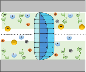
Figure 1. Schematic representing the flow induced by temperature gradient induced in (a) a brush-free nanochannel and (b) a backbone-charged PE-brush-grafted nanochannel. It shows a situation where the EOS component of the flow ( $u_{EOS}$) opposes the COS component of the flow (
 $u_{COS}$) and the thermal component of the flow (
 $u_T$) as the thermo-osmotically induced electric field is negative (i.e. directed from right to left). Of course, it is equally possible that the thermo-osmotically induced electric field is positive (i.e. directed left to right) and the EOS flow aids the COS component and the thermal component. Here
  $\lambda _{EDL}$ is the EDL thickness.
2.1. Modelling of pH-responsive PE brushes using augmented strong stretching theory
The brush configuration and electrostatics are modelled using our recently developed augmented SST which improves the existing SST (Lyatskaya et al. Reference Lyatskaya, Leermakers, Fleer, Zhulina and Birshtein1995; Zhulina & Borisov Reference Zhulina and Borisov1997; Zhulina et al. Reference Zhulina, Klein Wolterink and Borisov2000; Lebedeva et al. Reference Lebedeva, Zhulina and Borisov2017) by taking into account the effects of excluded volume effect and a more generic mass action law. In this model, the total free energy functional ( $F$) of the PE brush molecule is minimized to obtain the equilibrium configuration. The total free energy functional of the PE brush molecule is given by
 \begin{equation} \frac{F}{k_{B}T}=\frac{F_{els}}{k_{B}T}+\frac{F_{EV}}{k_{B}T}+ \frac{F_{elec}}{k_{B}T}+\frac{F_{EDL}}{k_{B}T}+\frac{F_{ion}}{k_{B}T},\end{equation}
where  $F_{els}$ is the elastic contribution to the free energy,
  $F_{EV}$ is the energy associated with excluded volume effect,
  $F_{elec}$ is the electrostatic free energy,
  $F_{EDL}$ is the free energy associated with electrostatic energy of the brush-induced EDL,
  $F_{ion}$ is ionization free energy and
  $k_BT$ is the thermal energy. Kindly refer to our previous work (Sachar et al. Reference Sachar, Sivasankar and Das2019b) for detailed description and the step-by-step minimization procedure.
We minimize the net free energy (see (2.1)) by using the variational formalism in the presence of the following constraints:
 \begin{gather} N=\int_{{-}h}^{y'}\frac{\textrm{d} y}{\bar{U}}(y,y'), \end{gather}
 \begin{gather}N=\frac{1}{\sigma a^3}\int_{{-}h}^{H-h}\phi(y)\,{\textrm{d} y}. \end{gather}
Here,  $N$ is the number of monomers in a PE chain,
  $\bar {U}(y,y^\prime )={\textrm {d} y}/\textrm {d}n$ quantifies the local stretching of the chain at a location
  $y$ (the chain is characterized by the fact that its end is located at
  $y^\prime$), where
  $n$ is the order number of monomer unit. Also,
  $a, H, \phi (y), \sigma \sim {1}/{\ell ^2}$ (
 $\ell$ is the separation between the adjacent PE grafting sites) are the Kuhn length, the brush height, dimensionless monomer distribution of the PE brushes, and the grafting density of the PE brushes, respectively. The variational minimization of (2.1) (see (Sachar et al. Reference Sachar, Sivasankar and Das2019b) for step-by-step details) provides the following governing equations describing the equilibrium behaviour of the system (the lower half of the nanochannel):
 \begin{gather} n_{A^-}=\frac{K_a'\gamma}{K_a'+n_{\textrm{H}^+,\infty}\exp\left(-\gamma a^3\dfrac{e\psi}{k_BT}\right)},\end{gather}
 \begin{gather} \left. \begin{array}{c@{}} \epsilon_{0}\epsilon_{r}\left(\dfrac{\textrm{d}^2\psi}{{\textrm{d} y}^2}\right)+e(n_+{-}n_-{+}n_{\textrm{H}^+}-n_{\textrm{OH}^-}-n_{A^-}\phi)=0 \quad ({-}h\leq y\leq{-}h+H),\\ \epsilon_{0}\epsilon_{r}\left(\dfrac{\textrm{d}^2\psi}{{\textrm{d} y}^2}\right)+e(n_+{-}n_-{+}n_{\textrm{H}^+}-n_{\textrm{OH}^-})=0 \quad ({-}h+H\leq y\leq 0), \end{array}\right\} \end{gather}
 \begin{gather} n_{{\pm}}=n_{{\pm} ,\infty}\exp \left({\mp}\frac{e\psi}{k_BT}\right), \end{gather}
 \begin{gather}n_{\textrm{H}^+}=n_{\textrm{H}^+,\infty}\exp \left(-\frac{e\psi}{k_BT}\right), \end{gather}
 \begin{gather}n_{\textrm{OH}^-}=n_{\textrm{OH}^-,\infty}\exp \left(\frac{e\psi}{k_BT}\right), \end{gather}
 \begin{align} \nonumber\\ \phi (y)& = \frac{\nu}{3\omega}\left[\left\{1+\kappa_B^2\left(\lambda-(y+h)^2 +\beta\frac{K_a'\gamma}{K_a'+n_{\textrm{H}^+,\infty}\exp\left(-\gamma a^3\dfrac{e\psi}{k_BT}\right)}\psi \right.\right.\right.\nonumber\\ & \quad {-\rho\left(1-\frac{K_a'}{K_a'+n_{\textrm{H}^+,\infty}\exp\left(-\gamma a^3\dfrac{e\psi}{k_BT}\right)}\right)\ln\left(1-\frac{K_a'}{K_a'+n_{\textrm{H}^+,\infty}\exp\left(-\gamma a^3\dfrac{e\psi}{k_BT}\right)}\right)}\nonumber\\ &\quad {-\rho\frac{K_a'}{K_a'+n_{\textrm{H}^+,\infty}\exp\left(-\gamma a^3\dfrac{e\psi}{k_BT}\right)}\ln\left(\frac{K_a'}{K_a'+n_{\textrm{H}^+,\infty}\exp\left(-\gamma a^3\dfrac{e\psi}{k_BT}\right)}\right)}\nonumber\\ &\quad \left.\left.{\left.-\rho\frac{K_a'}{K_a'+n_{\textrm{H}^+,\infty}\exp\left(-\gamma a^3\dfrac{e\psi}{k_BT}\right)}\ln\left(\frac{n_{\textrm{H}^+,\infty}}{K_a'}\right) \right)}\right\}^{1/2}-1\right], \end{align}
 \begin{gather} \bar{U}(y,y')=\frac{\pi}{2N}\sqrt{{(y'+h)}^{2}-(y+h)^2}, \end{gather}
 \begin{gather}(q_{net})_{H=H_0}=0, \end{gather}
 \begin{gather}q_{net}=\frac{e}{\sigma}\int_{{-}h}^{0}(n_+{-}n_-{+}n_{\textrm{H}^+}-n_{\textrm{OH}^-}-\phi n_{A^-})\,{\textrm{d} y}, \end{gather}
 \begin{gather}g(y)=\frac{(y+h)}{\sigma Na^3}\left[\frac{\phi({-}h+H)}{\sqrt{H^2-(y+h)^2}}- \int_{y}^{H-h}\frac{\textrm{d}\phi(y')}{{\textrm{d} y}'}\frac{{\textrm{d} y}'}{\sqrt{{(y'+h)}^2-(y+h)^2}}\right]. \end{gather}
Equation (2.4) gives the relation for the number density of the  $A^-$ ion (
 $n_{A^-}$) produced by acid-like disassociation of HA (here HA represents the acid) on the brush backbone. In (2.4),
  $K_a'=10^3N_{A}K_a$, where
  $K_a$ is the ionization constant of the acid-like disassociation of HA,
  $n_{\textrm {H}^+,\infty }=10^3N_{A}c_{\textrm {H}^+,\infty }$ (
 $c_{\textrm {H}^+,\infty }$ is the bulk concentration of the H
 $^+$ ions in Molars and can be related to
  $\textrm {pH}_\infty$ as
  $c_{\textrm {H}^+,\infty }=10^{-\textrm {pH}_\infty }, N_A$ is the Avagdro number),
  $e$ is the elementary charge and
  $\gamma$ is the polyelectrolyte chargeable sites (PCS) density in units of
  $1/\textrm {m}^3$. Equation (2.5) provides the distribution of the EDL electrostatic potential
  $\psi$ for the bottom half of the nanochannel (
 $-h\le y\le 0$). Equations (2.6)–(2.8) express the ion number densities through the Boltzmann distributions. Here,
  $n_i$ and
  $n_{i,\infty } (=10^3 N_A c_{i,\infty }$, where
  $c_{i,\infty }$ is the bulk concentration of ion
  $i$ in Molars) represent the number density and bulk number density for ion
  $i$ [where
  $i=\pm$, H
 $^+$, OH
 $^-$],
  $\epsilon _0$ is the permittivity of free space and
  $\epsilon _r$ is relative permittivity of the electrolyte solution. Equation (2.9) provides the monomer distribution profile and
  $\kappa _B^2={9\pi ^2\omega }/{8N^2a^2\nu ^2}, \rho ={8a^2N^2}/{3\pi ^2}, \lambda =-\lambda _1\rho =-\lambda _1({8a^2N^2}/{3\pi ^2}) (\lambda _1$ is the Lagrange multiplier associated with the constraint expressed in (2.3), and
  $\nu $ and
  $\omega $ are the virial coefficients associated with excluded volume free energy and
  $\beta ={8N^2ea^5}/{3\pi ^2k_BT}$. Equation (2.10) provides the condition of local stretching. Equation (2.11) considers the net unbalanced charge
  $q_{net}$ in the system (see (2.12)) and provides a condition for quantifying the equilibrium brush height
  $H_0$. Finally, (2.13) quantifies the normalized chain end distribution (
 $g(y')$) that also satisfies the condition
  ${\int _{-h}^{H-h}g(y^\prime )\,{\textrm {d} y}^\prime =1}$. The brush configuration and electrostatics (which eventually provide the brush height, monomer distribution and the brush-induced EDL distribution) are finally obtained by solving ((2.4)–(2.13)) in the presence of the following boundary condition for the EDL electrostatics (assuming an uncharged grafting surface):
 \begin{align} &(\psi)_{y=({-}h+H)^-}=(\psi)_{y=({-}h+H)^+},\quad \left(\frac{\textrm{d}\psi}{\textrm{d} y}\right)_{y=({-}h+H)^-}=\left(\frac{\textrm{d}\psi}{\textrm{d} y}\right)_{y=({-}h+H)^+},\nonumber\\ &\quad \left(\frac{\textrm{d}\psi}{\textrm{d} y}\right)_{y={-}h}=0,\quad \left(\frac{\textrm{d}\psi}{\textrm{d} y}\right)_{y=0}=0. \end{align}
Here the superscript ‘ $+$’ refers to the location of the tip of the brush when approached from the brush-free bulk side and the superscript ‘
 $-$’ refers to the location of the tip of the brush when approached from the brush side.
2.2. TOS transport in brush-grafted nanochannels
Thermo-osmotic flow, induced by a temperature gradient ( $\boldsymbol {\nabla } T$) across the nanochannel length (
 $L$), is considered to be unidirectional, steady and fully developed based on space charge theory (SCT) (Gross & Osterle Reference Gross and Osterle1968; Peters et al. Reference Peters, Van Roij, Bazant and Biesheuvel2016; Ryzhkov et al. Reference Ryzhkov, Lebedev, Solodovnichenko, Shiverskiy and Simunin2017, Reference Ryzhkov, Lebedev, Solodovnichenko, Minakov and Simunin2018). According to SCT, there exists a local equilibrium in the transverse direction at any location along the length of the channel. Here, we can apply the SCT to the ionic number density, the ionic and thermal fluxes, the EDL and the local flow field, as we consider the flow in a long nanochannel, i.e.
  $L\gg h$. We have also shown in our previous work that when a very small gradient of salt concentration is applied across this long nanochannel, the SCT is applicable (see the supplementary material of Jing & Das Reference Jing and Das2018). Similarly, for a very weak gradient in temperature applied in a long and thin nanochannel, the SCT will be applicable. The fluid transport in the presence of temperature gradient is governed by the Navier–Stokes (NS) equations which are expressed below. The pressure field (
 $p$), obtained from the
  $y$-momentum NS equation using the number density relations provided in (2.6)–(2.8), is as follows:
 \begin{equation} \left.\begin{array}{c@{}} \begin{aligned} & \dfrac{\partial p}{\partial y}+ e({n_+}-{n_-}+{n_{\textrm{H}^+}}-{n_{\textrm{OH}^-}}) \dfrac{\partial \psi}{\partial y} = 0\Rightarrow \dfrac{\partial p}{\partial y}\\ & \quad ={-}k_BT ({n_+}-{n_-}+{n_{\textrm{H}^+}}-{n_{\textrm{OH}^-}})\dfrac{\partial \bar{\psi}}{\partial y}\Rightarrow \end{aligned}\\ p = p_{atm}+2k_BT({n_{+,\infty}}+{n_{\textrm{H}^+,\infty}}){(\cosh(\bar{\psi})-\cosh(\overline{\psi_c})}) \end{array}\right\}.\end{equation}
In (2.15),  $\bar {\psi }={e\psi }/{k_BT}, \bar{\psi}_c = (\bar{\psi})_{(y = 0)}, p_{atm}$ is the atmospheric pressure,
  $n_\infty =10^3N_Ac_{\infty} , n_{\textrm {H}^+,\infty } =10^3N_A10^{-\textrm {pH}_\infty }$ and
  $n_{\textrm {OH}^-,\infty }= 10^3N_A10^{-p \textrm {OH}_\infty }$, where
  $p \textrm {OH}_{\infty }=14-\textrm {pH}_{\infty }$. The relations between different bulk number densities are
  $n_{+,\infty }=n_{\infty }, n_{-,\infty }=n_{\infty }+n_{\textrm {H}^+,\infty }-n_{\textrm {OH}^-,\infty }$. The axial pressure gradient
  ${\partial p}/{\partial x}$ induced by the presence of temperature gradient is given by
 \begin{align} &\frac{\partial p}{\partial x} = 2k_BT\left[\left( \frac{\textrm{d}n_\infty}{\textrm{d} x} + \frac{\textrm{d}n_{\textrm{H}^+,\infty}}{\textrm{d} x}\right)\right.{(\cosh(\bar{\psi})-\cosh(\bar{\psi}_c))}+({n_{\infty}}\nonumber\\ &\quad +{n_{\textrm{H}^+,\infty}})\left.\left({\sinh(\bar{\psi}) \frac{\partial\bar{\psi}}{\partial x}-\sinh(\bar{\psi}_c) \frac{\partial\bar{\psi}_c}{\partial x}}\right) \right]\nonumber\\ &\quad +2k_B\left( \frac{\textrm{d}T}{\textrm{d} x}\right) (n_\infty+n_{\textrm{H}^+,\infty}){(\cosh(\bar{\psi})-\cosh(\bar{\psi}_{c}))}. \end{align}
 The  $x$-momentum equation in the bottom half-channel (
 $-h \leq y \leq 0$) which provides the equation governing the TOS velocity is expressed as:
 \begin{align} \left. \begin{array}{c@{}} \displaystyle\eta\dfrac{\partial^2u}{\partial y^2}=\dfrac{\partial p}{\partial x}+\dfrac{\eta}{\kappa_d}u-e(n_+{-}n_-{+}n_{\textrm{H}^+}-n_{\textrm{OH}^-})\left(E-\dfrac{\partial\psi}{\partial x}\right) \quad ({-}h\leq y\leq{-}h+H_0)\\ \displaystyle\eta\dfrac{\partial^2u}{\partial y^2}=\dfrac{\partial p}{\partial x}-e(n_+{-}n_-{+}n_{\textrm{H}^+}-n_{\textrm{OH}^-})\left(E-\dfrac{\partial\psi}{\partial x}\right) \quad ({-}h+H_0\leq y\leq 0) \end{array}\right\}. \end{align}
In the above equation,  $u, \eta , {\partial p}/{\partial x}, E, {\eta }/{\kappa _d}$ represents the fluid velocity, viscosity, induced pressure gradient (see (2.16)), induced electric field due to the TOS flow and the per unit volume drag coefficient respectively. Here,
  $\kappa _d = a^2/\phi ^2=a^2 ({H_0}/{\sigma a^3 N \bar {\phi }})^2$, where
  $\bar {\phi }=({\phi H_0}/{\sigma a^3 N})$ is the normalized monomer distribution obtained from the SST formulation. Following the study of De Gennes (Reference De Gennes1976a) and Freed & Edwards (Reference Freed and Edwards1974), it is seen that
  $\kappa _d \sim K^{-2}$, where
  $K^{-1}$ is the length across which the flow inside a polymer coil is screened in a semidilute polymer solution. Also,
  $K \sim \phi / a$, which results in
  $\kappa _d \sim a^2/\phi ^2$.
Using (2.17) at  $y=0$, where
  $p =p_{atm}$ and
  $\psi = \psi _c$, we can obtain the expression for
  ${\partial {\psi }_{c}}/{\partial x}$ as follows:
 \begin{equation} \left. \begin{array}{c} \displaystyle\eta\left(\dfrac{\partial^2u}{\partial y^2}\right)_{(y=0)}={-}e(n_+{-}n_-{+}n_{\textrm{H}^+}-n_{\textrm{OH}^-})_{(y=0)}\left(E- \dfrac{\partial\psi_c}{\partial x}\right)\\ \displaystyle\Rightarrow \dfrac{\partial {\psi}_{c}}{\partial x} = E-\dfrac{1}{-e(n_+{-}n_-{+}n_{\textrm{H}^+}-n_{\textrm{OH}^-})_{(y=0)}} \eta\left(\dfrac{\partial^2u}{\partial y^2}\right)_{(y=0)} \end{array}\right\}. \end{equation}
Using the chain rule, the terms  ${\partial {\psi }}/{\partial x}$, and
  ${\partial \bar {\psi }_{c}}/{\partial x}$ (where
  $\bar {\psi }_{c}={e\psi _c}/{k_BT}$) are written as
 \begin{gather} \frac{\partial {\psi}}{\partial x} = \frac{k_BT}{e}\frac{\partial \bar{\psi}}{\partial x}+\frac{k_B\bar{\psi}}{e}\frac{\partial T}{\partial x}, \end{gather}
 \begin{gather}\frac{\partial \overline{\psi_c}}{\partial x} = \frac{e}{k_BT}\frac{\partial {\psi}_{c}}{\partial x}-\frac{\overline{\psi_c}}{T}\frac{\partial T}{\partial x}. \end{gather}
Using (2.6)–(2.8), (2.16)–(2.20), we can eventually express the equations governing the TOS velocity in dimensionless form as
 \begin{equation} \left.\begin{array}{c@{}} \begin{aligned} \dfrac{\textrm{d}^2\bar{u}}{\textrm{d}\bar{y}^2}- \left(\dfrac{\textrm{d}^2\bar{u}}{\textrm{d}\bar{y}^2}\right)_{(\bar{y}=0)} & = {\bar{n}'}\bar{\kappa}^2(\cosh(\bar{\psi})-\cosh(\overline{\psi_c}))+ \dfrac{L}{T}\dfrac{\textrm{d}T}{\textrm{d} x}\bar{\kappa}^2(\cosh(\bar{\psi})\\ & \quad -\cosh(\overline{\psi_c})- \bar{\psi} \sinh(\bar{\psi})+ \overline{\psi_c} \sinh(\overline{\psi_c}))+ \dfrac{h^2}{\kappa_d}\bar{u}\\ & \quad +\bar{\kappa}^2{(\sinh(\bar{\psi})-\sinh(\overline{\psi_c}))} \bar{E} \quad ({-}1\leq \bar{y}\leq{-}1+\bar{H}_0), \end{aligned}\\ \begin{aligned} \dfrac{\textrm{d}^2\bar{u}}{\textrm{d}\bar{y}^2}- \left(\dfrac{\textrm{d}^2\bar{u}}{\textrm{d}\bar{y}^2}\right)_{(\bar{y}=0)} & = {\bar{n}'}\bar{\kappa}^2{(\cosh(\bar{\psi})-\cosh(\overline{\psi_c}))} +\dfrac{L}{T}\dfrac{\textrm{d}T}{\textrm{d} x}\bar{\kappa}^2(\cosh(\bar{\psi})\\ & \quad -\cosh(\overline{\psi_c})- \bar{\psi}\sinh(\bar{\psi})+ \overline{\psi_c}\sinh(\overline{\psi_c}))\\ & \quad + \bar{\kappa}^2{(\sinh(\bar{\psi})-\sinh(\overline{\psi_c}))}\bar{E} \quad ({-}1+\bar{H}_0\leq \bar{y}\leq 0). \end{aligned} \end{array}\right\} \end{equation}
Here,  $\bar{y} = y/h, \bar{H_0} = H_0/h, \bar {u}=u/U, U = {\epsilon _0 \epsilon _r (k_BT)^2}/{e^2L\eta }, \bar {E}=E/E_0, E_0 = $
 ${k_BT}/{eL}$,
  $\bar{\psi}={e \psi }/{k_BT}$,
  $\bar {n}'={L(\boldsymbol {\nabla } n_\infty +\boldsymbol {\nabla } n_{\textrm {H}^+,\infty })}/{(n_\infty +n_{\textrm {H}^+,\infty })}$,
  $\bar {\kappa }^2=({\kappa }h)^2$, and
  $\kappa ^2 = {1}/{\lambda _{EDL}^2}={2 e^2 (n_\infty + n_{\textrm {H}^+,\infty })}/ {\epsilon _0 \epsilon _r k_B T}$. Equation (2.21) will get simplified as the symmetry condition at the channel centerline will eventually lead to
  $({\textrm {d}^2\bar {u}}/{\textrm {d}\bar {y}^2})_{(\bar {y}=0)}=0$. In (2.21), the centreline potential
  $\psi _c$ is obtained from the SST formulation. The electrostatic potential throughout the channel (including
  $\psi _c$) is obtained by solving (2.4)–(2.13) in the presence of the boundary condition given in (2.14a–d). Equation (2.21) shows that the TOS velocity is governed by three driving forces: a COS force due to the concentration gradient, a TOS force component due the temperature gradient, and a component due to the induced electric field. The first two terms on the right-hand side of (2.21) are contributions due to the induced axial pressure gradient. These pressure gradient based terms arise because of the change in osmotic pressure along the length of the channel due to (1) the Soret effect induced concentration gradient, and (2) the applied temperature gradient. The first term on the right-hand side of (2.21) represents the COS contribution which is due to the interaction of EDL mobile ions with the induced axial concentration gradient. Please note that in the COS term,
  $\overline {n^\prime }={L(\boldsymbol {\nabla } n_\infty +\boldsymbol {\nabla } n_{\textrm {H}^+,\infty })}/{(n_\infty +n_{\textrm {H}^+,\infty })}$ represents the non-dimensional concentration gradient and
  ${\bar {\kappa }}^2{(\cosh (\bar {\psi })-\cosh (\overline {\psi _c}))}$ represents the net concentration of mobile ions in the EDL. The second term on the right-hand side of (2.21) represents the TOS component which is due to interaction of the EDL mobile ions with the applied temperature gradient. Please note that in the TOS term,
  $({L}/{T})({\textrm {d}T}/{\textrm {d} x})$ represents the non-dimensional temperature gradient and
  ${\bar {\kappa }}^2{(\cosh (\bar {\psi })-\cosh (\overline {\psi _c})-\bar {\psi }\sinh (\bar {\psi })+\overline {\psi _c}\sinh (\overline {\psi _c}))}$ represents the contribution due to the EDL mobile ions. The term
  $({h^2}/{\kappa _d})\bar {u}$ (please see the third term on the right-hand side of the first equation of (2.21)) represents the drag force induced by the presence of the PE brushes. Finally, the last term on the right-hand side of (2.21) represents the EOS body force term which is clearly the effect of the induced electric field
  $(\bar {E})$ on the EDL charge densities. It is to be noted that in the EOS term,
  $\bar {E}$, is the dimensionless induced electric field and
  ${\bar {\kappa }}^2{(\sinh (\bar {\psi })-\sinh (\overline {\psi _c}))}$ represents the non-dimensional EDL mobile charge densities.
Equation (2.21) is solved in the presence of the following boundary conditions:
 \begin{align} &(\bar{u})_{\bar{y}={-}1}=0; \quad \left(\frac{\partial \bar{u}}{\partial\bar{y}}\right)_{\bar{y}=0}=0; \quad (\bar{u})_{\bar{y}=({-1+\bar{H_0}})^-}= (\bar{u})_{\bar{y}=({-1+\bar{H_0}})^+}; \nonumber\\ &\quad \left(\frac{\partial\bar{u}}{\partial\bar{y}}\right)_{\bar{y}=({-}1+\bar{H_0})^-}= \left(\frac{\partial\bar{u}}{\partial\bar{y}} \right)_{\bar{y}=({-}1+\bar{H_0})^+}. \end{align}
 The dimensionless electric field,  $\bar {E}$, has to be calculated in order to obtain the dimensionless velocity field
  $\bar {u}$ (see (2.21)). The induced electric field
  $E$ is obtained from the condition of zero overall current in the system (as there is no externally employed electric field), i.e.
 \begin{equation} \int_{{-}h}^h(J_+{+}J_{\textrm{H}^+}-J_--J_{\textrm{OH}^-})\,{\textrm{d} y}=0,\end{equation}
where  $J_i$ is the flux of the ion
  $i$ (
$i$ ( $i = \pm , \textrm {H}^+,\textrm {OH}^-$). Expressions for these fluxes are as follows:
 \begin{equation} \left. \begin{array}{c@{}} \displaystyle J_\pm{=}{-}D_\pm \left[ \dfrac{\textrm{d}n_\pm}{\textrm{d} x} \pm \dfrac{e}{k_BT}n_\pm \left(\dfrac{\textrm{d}\psi}{\textrm{d} x} - E\right)+\dfrac{Q_\pm}{RT^2}n_\pm \dfrac{\textrm{d}T}{\textrm{d} x}\right]+n_\pm u,\\ \displaystyle J_{\textrm{H}^{+}}={-}D_{\textrm{H}^+} \left[\dfrac{\textrm{d}n_{\textrm{H}^+}}{\textrm{d} x} +\dfrac{e}{k_BT}n_{\textrm{H}^+} \left(\dfrac{\textrm{d}\psi}{\textrm{d} x} - E\right)+\dfrac{Q_{\textrm{H}^+}}{RT^2}n_{\textrm{H}^+} \dfrac{\textrm{d}T}{\textrm{d} x}\right]+n_{\textrm{H}^+} u,\\ \displaystyle J_{\textrm{OH}^{-}}={-}D_{\textrm{OH}^-} \left[\dfrac{\textrm{d}n_{\textrm{OH}^-}}{\textrm{d} x} -\dfrac{e}{k_BT}n_{\textrm{OH}^-}\left(\dfrac{\textrm{d}\psi}{\textrm{d} x} - E\right)+\dfrac{Q_{\textrm{OH}^-}}{RT^2}n_{\textrm{OH}^-} \dfrac{\textrm{d}T}{\textrm{d} x}\right]+n_{\textrm{OH}^-} u. \end{array} \right\}\end{equation}
It is to be noted that the diffusive component of the flux in (2.24) can be expressed as:
 \begin{equation} -D_i \left(\frac{\textrm{d}n_i}{\textrm{d} x}\right)={-}D_i \exp \left(\frac{-z_i e\psi}{k_BT}\right) \left[\frac{\textrm{d}n_{i,\infty}}{\textrm{d} x} - n_{i,\infty} \frac{z_i e}{k_BT} \left(\frac{\textrm{d}\psi}{\textrm{d} x}\right) + n_{i,\infty} \frac{z_ie \psi}{k_BT^2}\left(\frac{\textrm{d}T}{\textrm{d} x}\right)\right].\end{equation}
In the above equations,  $D_i, Q_i, z_i$ are, respectively, the diffusivity, heat of transport, and valence of ion
  $i$ (
$i$ ( $i=\pm ,\textrm {H}^+,\textrm {OH}^-$). Using (2.6)–(2.8), (2.24) and (2.25) in (2.23), we can eventually obtain the dimensionless thermo-osmotically induced electric field as:
 \begin{align} \bar{E}&=
\frac{\begin{aligned} & -L P_+ \boldsymbol{\nabla} T
\int_{{-}1}^{1} [R_{+}\boldsymbol{\nabla}
\bar{n}_{+,\infty}\exp(-\bar{\psi})-R_{-}\boldsymbol{\nabla}
\bar{n}_{-,\infty}\exp(\bar{\psi})+{R}_{\textrm{H}^+}\boldsymbol{\nabla}
\bar{n}_{\textrm{H}^+,\infty}\exp(-\bar{\psi})\\ & \quad
-R_{\textrm{OH}^-,\infty} \boldsymbol{\nabla}
\bar{n}_{\textrm{OH}^-,\infty}\exp(\bar{\psi})]\,
\textrm{d}\bar{y}\end{aligned}}{\begin{aligned} & T
\int_{{-}1}^{1}
[R_+\bar{n}_{+,\infty}\exp(-\bar{\psi})+R_-\bar{n}_{-,\infty}\exp(\bar{\psi})+
R_{\textrm{H}^+,\infty}
\bar{n}_{\textrm{H}^+,\infty}\exp(-\bar{\psi})\\ & \quad +
R_{\textrm{OH}^-,\infty}
\bar{n}_{\textrm{OH}^-,\infty}\exp(\bar{\psi})]\,
\textrm{d}\bar{y}\end{aligned}} \nonumber\\ &\quad
+\frac{\begin{aligned} & L \boldsymbol{\nabla} T
\int_{{-}1}^{1}[R_+ \bar{n}_+(\bar{Q}_+{+}\bar{\psi} )-R_-
\bar{n}_-(\bar{Q}_-- \bar{\psi} )+R_+
\bar{n}_{\textrm{H}^+}(\bar{Q}_{\textrm{H}^+} +\bar{\psi}
)\\ & \quad -R_{\textrm{OH}^-}
\bar{n}_{\textrm{OH}^-}(\bar{Q}_{\textrm{OH}^-} -
\bar{\psi} )]\,
\textrm{d}\bar{y}\end{aligned}}{\begin{aligned} & T
\int_{{-}1}^{1}
[R_+\bar{n}_{+,\infty}\exp(-\bar{\psi})+R_-\bar{n}_{-,\infty}\exp(\bar{\psi})+
R_{\textrm{H}^+,\infty}
\bar{n}_{\textrm{H}^+,\infty}\exp(-\bar{\psi})\\ & \quad +
R_{\textrm{OH}^-,\infty}
\bar{n}_{\textrm{OH}^-,\infty}\exp(\bar{\psi})]\,
\textrm{d}\bar{y}\end{aligned}}\nonumber\\ &\quad
+\frac{\begin{aligned} & Pe \int_{{-}1}^{1}
\bar{u}[-\bar{n}_{+,\infty}\exp(-\bar{\psi})+\bar{n}_{-,\infty}\exp(\bar{\psi})-
\bar{n}_{\textrm{H}^+,\infty}\exp(-\bar{\psi})\\ & \quad +
\bar{n}_{\textrm{OH}^-,\infty}\exp(\bar{\psi})]\,
\textrm{d}\bar{y}\end{aligned}}{\begin{aligned} &
\int_{{-}1}^{1}
[R_+\bar{n}_{+,\infty}\exp(-\bar{\psi})+R_-\bar{n}_{-,\infty}\exp(\bar{\psi})+
R_{\textrm{H}^+,\infty}
\bar{n}_{\textrm{H}^+,\infty}\exp(-\bar{\psi})\\ & \quad +
R_{\textrm{OH}^-,\infty}
\bar{n}_{\textrm{OH}^-,\infty}\exp(\bar{\psi})]\,
\textrm{d}\bar{y}\end{aligned}}\nonumber\\
&=\bar{E}_{ion}+\bar{E}_t+\bar{E}_{osm}=\sum_i
(\bar{E}_{ion,i}+\bar{E}_{t,i}+\bar{E}_{osm,i}).
\end{align}
\begin{align} \bar{E}&=
\frac{\begin{aligned} & -L P_+ \boldsymbol{\nabla} T
\int_{{-}1}^{1} [R_{+}\boldsymbol{\nabla}
\bar{n}_{+,\infty}\exp(-\bar{\psi})-R_{-}\boldsymbol{\nabla}
\bar{n}_{-,\infty}\exp(\bar{\psi})+{R}_{\textrm{H}^+}\boldsymbol{\nabla}
\bar{n}_{\textrm{H}^+,\infty}\exp(-\bar{\psi})\\ & \quad
-R_{\textrm{OH}^-,\infty} \boldsymbol{\nabla}
\bar{n}_{\textrm{OH}^-,\infty}\exp(\bar{\psi})]\,
\textrm{d}\bar{y}\end{aligned}}{\begin{aligned} & T
\int_{{-}1}^{1}
[R_+\bar{n}_{+,\infty}\exp(-\bar{\psi})+R_-\bar{n}_{-,\infty}\exp(\bar{\psi})+
R_{\textrm{H}^+,\infty}
\bar{n}_{\textrm{H}^+,\infty}\exp(-\bar{\psi})\\ & \quad +
R_{\textrm{OH}^-,\infty}
\bar{n}_{\textrm{OH}^-,\infty}\exp(\bar{\psi})]\,
\textrm{d}\bar{y}\end{aligned}} \nonumber\\ &\quad
+\frac{\begin{aligned} & L \boldsymbol{\nabla} T
\int_{{-}1}^{1}[R_+ \bar{n}_+(\bar{Q}_+{+}\bar{\psi} )-R_-
\bar{n}_-(\bar{Q}_-- \bar{\psi} )+R_+
\bar{n}_{\textrm{H}^+}(\bar{Q}_{\textrm{H}^+} +\bar{\psi}
)\\ & \quad -R_{\textrm{OH}^-}
\bar{n}_{\textrm{OH}^-}(\bar{Q}_{\textrm{OH}^-} -
\bar{\psi} )]\,
\textrm{d}\bar{y}\end{aligned}}{\begin{aligned} & T
\int_{{-}1}^{1}
[R_+\bar{n}_{+,\infty}\exp(-\bar{\psi})+R_-\bar{n}_{-,\infty}\exp(\bar{\psi})+
R_{\textrm{H}^+,\infty}
\bar{n}_{\textrm{H}^+,\infty}\exp(-\bar{\psi})\\ & \quad +
R_{\textrm{OH}^-,\infty}
\bar{n}_{\textrm{OH}^-,\infty}\exp(\bar{\psi})]\,
\textrm{d}\bar{y}\end{aligned}}\nonumber\\ &\quad
+\frac{\begin{aligned} & Pe \int_{{-}1}^{1}
\bar{u}[-\bar{n}_{+,\infty}\exp(-\bar{\psi})+\bar{n}_{-,\infty}\exp(\bar{\psi})-
\bar{n}_{\textrm{H}^+,\infty}\exp(-\bar{\psi})\\ & \quad +
\bar{n}_{\textrm{OH}^-,\infty}\exp(\bar{\psi})]\,
\textrm{d}\bar{y}\end{aligned}}{\begin{aligned} &
\int_{{-}1}^{1}
[R_+\bar{n}_{+,\infty}\exp(-\bar{\psi})+R_-\bar{n}_{-,\infty}\exp(\bar{\psi})+
R_{\textrm{H}^+,\infty}
\bar{n}_{\textrm{H}^+,\infty}\exp(-\bar{\psi})\\ & \quad +
R_{\textrm{OH}^-,\infty}
\bar{n}_{\textrm{OH}^-,\infty}\exp(\bar{\psi})]\,
\textrm{d}\bar{y}\end{aligned}}\nonumber\\
&=\bar{E}_{ion}+\bar{E}_t+\bar{E}_{osm}=\sum_i
(\bar{E}_{ion,i}+\bar{E}_{t,i}+\bar{E}_{osm,i}).
\end{align}
Here  $Pe = {UL}/({D_++D_-+D_{\textrm {H}^+}-D_{\textrm {OH}^-}}),\ R_i = {D_i}/({{D_++D_-+D_{\textrm {H}^+}-D_{\textrm {OH}^-}}}),$
 $\bar {Q}_i = Q_{i}/RT$,
  $P_i={Q_i}/{2RT}, R=k_B N_A$, and
  $\boldsymbol {\nabla } n_{i,\infty } = - P_i ({\boldsymbol {\nabla } T}/{T}) n_{i,\infty }$ represents, respectively, the Péclet number, normalized diffusion coefficient, normalized heat of transport, Soret coefficient, universal gas constant and the gradient in the bulk concentration of ion
  $i$ (
$i$ ( $i =\pm ,\textrm {H}^+,\textrm {OH}^-$). Also,
  $\boldsymbol {\nabla } \bar {n}_{i,\infty } = {\boldsymbol {\nabla } n_{i,\infty }}/{\boldsymbol {\nabla } n_{+,\infty }}, \bar {n}_i={n_i}/{n_{+,\infty }}, \bar {n}_{i,\infty }={n_{i,\infty }}/{n_{+,\infty }}$. The ionic (
 $\bar {E}_{ion}$), the thermal (
 $\bar {E}_t$) and the osmotic (
 $\bar {E}_{osm}$) components of the induced dimensionless electric field are expressed as follows (from (2.26)):
 \begin{gather} \bar{E}_{ion}=\frac{\begin{aligned} & -L P_+ \boldsymbol{\nabla} T \int_{{-}1}^{1} [R_{+}\boldsymbol{\nabla} \bar{n}_{+,\infty}\exp(-\bar{\psi})-R_{-}\boldsymbol{\nabla} \bar{n}_{-,\infty}\exp(\bar{\psi})\\ & \quad +{R}_{\textrm{H}^+}\boldsymbol{\nabla} \bar{n}_{\textrm{H}^+,\infty}\exp(-\bar{\psi})-R_{\textrm{OH}^-,\infty} \boldsymbol{\nabla} \bar{n}_{\textrm{OH}^-,\infty}\exp(\bar{\psi})]\, \textrm{d}\bar{y}\end{aligned}}{\begin{aligned} & T \int_{{-}1}^{1} [R_+\bar{n}_{+,\infty}\exp(-\bar{\psi})+R_-\bar{n}_{-,\infty}\exp(\bar{\psi})+ R_{\textrm{H}^+,\infty} \bar{n}_{\textrm{H}^+,\infty}\exp(-\bar{\psi})\\ & \quad + R_{\textrm{OH}^-,\infty} \bar{n}_{\textrm{OH}^-,\infty}\exp(\bar{\psi})]\, \textrm{d}\bar{y} \end{aligned}}, \end{gather}
 \begin{gather}\bar{E}_{t}=\frac{\begin{aligned} & L \boldsymbol{\nabla} T \int_{{-}1}^{1}[R_+ \bar{n}_+(\bar{Q}_+{+}\bar{\psi} )-R_- \bar{n}_-(\bar{Q}_-- \bar{\psi} )+R_+ \bar{n}_{\textrm{H}^+}(\bar{Q}_{\textrm{H}^+} +\bar{\psi} )\\ & \quad -R_{\textrm{OH}^-} \bar{n}_{\textrm{OH}^-}(\bar{Q}_{\textrm{OH}^-} - \bar{\psi} )]\, \textrm{d}\bar{y}\end{aligned}}{\begin{aligned} & T\int_{{-}1}^{1} [R_+\bar{n}_{+,\infty}\exp(-\bar{\psi})+R_-\bar{n}_{-,\infty}\exp(\bar{\psi})+ R_{\textrm{H}^+,\infty} \bar{n}_{\textrm{H}^+,\infty}\exp(-\bar{\psi})\\ & \quad + R_{\textrm{OH}^-,\infty} \bar{n}_{\textrm{OH}^-,\infty}\exp(\bar{\psi})]\, \textrm{d}\bar{y}\end{aligned}}, \end{gather}
 \begin{gather}\bar{E}_{osm}=\frac{\begin{aligned} & Pe \int_{{-}1}^{1} \bar{u}[-\bar{n}_{+,\infty}\exp(-\bar{\psi})+\bar{n}_{-,\infty}\exp(\bar{\psi})- \bar{n}_{\textrm{H}^+,\infty}\exp(-\bar{\psi})\\ & \quad + \bar{n}_{\textrm{OH}^-,\infty}\exp(\bar{\psi})]\, \textrm{d}\bar{y}\end{aligned}}{\begin{aligned} & \int_{{-}1}^{1} [R_+\bar{n}_{+,\infty}\exp(-\bar{\psi})+R_-\bar{n}_{-,\infty}\exp(\bar{\psi})+ R_{\textrm{H}^+} \bar{n}_{\textrm{H}^+,\infty}\exp(-\bar{\psi})\\ & \quad + R_{\textrm{OH}^-} \bar{n}_{\textrm{OH}^-,\infty}\exp(\bar{\psi})]\, \textrm{d}\bar{y}\end{aligned}}. \end{gather}
Finally, please note that  $\bar {E}_{j,i}$ (
 $j=ion,~t,~osm$) represents the contribution of ion
  $i$ to the component
  $j$ of the induced electric field (see (2.26)). Using the integral expression for electric field obtained in (2.26), we replace the term
  $\bar {E}$ in last term in the right-hand side of (2.21) and solve the resulting integro-differential equation in
  $\bar {u}$ using the finite difference method. To solve this integro-differential equation we use the Newton–Raphson method, where we provide an initial guess for the electric field and then iteratively solve for the velocity field and the corresponding electric field. In this study, we use a grid size of
  $5 \times 10^{-4}$ nm, and the convergence criterion was set to a relative tolerance of
  $10^{-9}$ for
  $\bar {E}$.
In this work, we perform the minimization of the free energy to find the brush configuration. However, for calculation of the flow (which refers to a non-equilibrium scenario), we assume that this equilibrium configuration of the brush is not significantly affected by the presence of the flow. Following a study by Kim et al. (Reference Kim, Lobaskin, Gutsche, Kremer, Pincus and Netz2009), where they use mean-field theory to quantify the tilt angle of the polymer brush in the presence of shear flow, we find that the maximum tilt angle for the brushes for the nanochannel flow (with a maximum flow velocity of  $10^{-5}~$ m s
 $^{-1}$, as witnessed in previous studies Pennathur & Santiago Reference Pennathur and Santiago2005) is approximately
  $0.51^{\circ }$. For the present case, this maximum velocity is actually much smaller (with
  $U={\epsilon _0 \epsilon _r (k_BT)^2}/{e^2L\eta }$) (
 $\sim 10^{-7}$ to
  $10^{-8}$ m s
 $^{-1}$). This will imply that this tilt is even smaller. Under such conditions, it is safe to assume that the PE brush equilibrium configuration is not significantly affected by the flow. The detailed calculations for quantifying this tilt are provided in appendix B.
3. Results and discussions
3.1. Variation of the thermo-osmotically induced electric field
We characterize the TOS flow by studying the thermo-osmotically induced dimensionless electric field  $\bar {E}$ and the dimensionless flow velocity
  $\bar {u}$. We compare the results for three different cases of brush-grafted nanochannel and three corresponding cases of the brushless nanochannel. In the following discussions, the brushless cases are identified as ‘No-Brush’ case. More importantly, we assume that the walls of these brushless nanochannels have the same charge density (
 $\sigma _{c,eq}$) as that of the corresponding brush-grafted cases (where the walls are uncharged and the charges are distributed on the brushes). Of course,
  $\sigma _{c,eq}$ is expressed as
  $\sigma _{c,eq}=-e\int _{-h}^{-h+H}\phi n_{A^-} {\textrm {d} y}$ (see the theory section for definitions of
  $\phi$ and
  $n_{A^-}$).
Thermo-osmotically induced electric field  $\bar {E} (=\bar {E}_{ion}+\bar {E}_{osm}+\bar {E}_{t})$ has contributions from ionic component (
 $\bar {E}_{ion}$) associated with the conduction of various ions, osmotic component (
 $\bar {E}_{osm}$) associated with the downward migration of the electrolyte ions, and thermal component (
 $\bar {E}_{t}$) due to the thermal gradient induced migration of the ions. The variation of
  $\bar {E}$ (shown in figure 2) is explained in detail by analysing each component contributing to the overall electric field. First, we study the variation of ionic component (
 $\bar {E}_{ion}$) (see figure 3(a)) of the induced electric field with the salt concentration (
 $c_\infty$). The ionic component of the electric field is due to the conduction of the EDL mobile ions. This component depends on the diffusivities of the mobile ions and the concentration gradient that is caused by the applied temperature gradient (
 $\textrm {d}T/{\textrm {d} x}$) due to the Soret effect. This induced concentration gradient acts on the EDL mobile ions (co-ions and counterions) of different diffusivities resulting in this conduction-based component. Figure 3(a) shows the variation of
  $\bar {E}_{ion}$ for all six cases:
  $\bar {E}_{ion}$ decreases in magnitude with an increase in the salt concentration (
 $c_\infty$). This is partly due to a decrease in the magnitude of the electrostatic potential
  $\bar {\psi }$ (see figure 4 which shows the typical variation of
  $|\bar {\psi }|$ with salt concentration) of the PE-brush-supported EDL with an increasing salt concentration. Such a decrease is caused by an augmented screening of the PE charges by a large concentration of the EDL ions. Equivalently, this decrease can be justified by noting that for a given average charge density
  $\sigma _{c,eq}$ (see figure 5), the magnitude of
  $\bar {\psi }$ is
  $|\bar {\psi }|\propto \sigma _{c,eq}\lambda _{EDL}\propto \sigma _{c,eq}/\sqrt {c_\infty }$ (
 $\lambda _{EDL}$ is the average EDL thickness). Of course, for very small electrolyte concentration (small enough to make
  $\lambda _{EDL}$ large enough to ensure an overlap of the EDL), the increase in
  $c_\infty$ causes a relatively weak decrease in
  $|\bar {\psi }|$. This is clearly seen for both the brush-grafted nanochannels and the corresponding cases in brushless nanochannels. The significant difference in the EDL potential distribution across the nanochannel between the cases of PE brush-grafted channel and the brushless channel can be attributed to the distribution of the charges in each of these cases. For instance, for the brushless nanochannels, the EDL potential has a finitely large magnitude (see figure 4(b)) only at locations near the walls of the nanochannel stemming from the fact that the charges (that induce the EDL) are localized at the walls. On the other hand, for the brush-grafted nanochannels, the PE brush charges are distributed along the brushes and hence the finitely large magnitude of the EDL potential is found to be distributed across the height of the channel (see figure 4(a)). It is also important to note that because of the localization of the charge on the walls for brush-free nanochannels, for the same charge density
  $\sigma _{c,eq}$, the EDL potential decreases sharply away from the wall (stronger near the wall and very weak away from the wall). However, for the brush-grafted nanochannels, the EDL potential decays much more slowly away from the wall owing to the PE charge distribution. In figure 5, we observe a monotonic increase in the magnitude of the charge density with increasing salt concentration. This charge density depends on the number of negative ions generated on the backbone of the PE brushes due to the ionization of the brushes. As the salt concentration increases, the EDL potential decreases due to an enhanced screening of the PE brush charge. This leads to a decrease in the local
  $\textrm {H}^+$ ion concentration (
 $n_H = n_{\textrm {H}^+,\infty }\exp (-\bar {\psi })$), which in turn leads to increased ionization of the brush. This increased ionization will lead to an increase in surface charge density. Similarly, with an increase in the grafting density (or decrease in
  $\ell$), we witness an increase in the number of PE chains grafted per unit area. This means an increase in the total charge per unit area, and hence we witness an increased surface charge density. Also, with increasing pH of the solution, we witness an increase in the magnitude of surface charge density. This is due to a decrease in
  $\textrm {H}^+$ ion concentration in the medium which increases the ionization of the PE brush.

Figure 2. Thermo-osmotically induced electric field due to the applied temperature gradient of  $\boldsymbol {\nabla } T=\textrm {d}T/{\textrm {d} x}= 20~\textrm {Km}^{-1}$. The parameters used in obtaining this electric field are:
  $k_B = 1.38 \times 10^{-23}$
  $\textrm {JK}^{-1}, T = 298\ \textrm {K}, e = 1.6\times 10^{-19}\ \textrm {C}$ (elementary charge),
  $\epsilon _0 = 8.8 \times 10^{-12}\ \textrm {Fm}^{-1}$ (permittivity of free space),
  $\epsilon _r = 79.8$ (relative permittivity of water),
  $N = 400, h = 100\ \textrm {nm}, L = 0.05\ \textrm {m}, a = 1$ nm (Kuhn length),
  $\gamma a^3=1, pK_a = 3.5, \nu = 0.5, \omega = 0.1$. Other parameters are
  $Q_+ = 3460\ \textrm {J}\ \textrm {mol}^{-1}, Q_- = 530 \ \textrm {J}\ \textrm {mol}^{-1}, Q_{\textrm {H}^+} = 13.3 \times 10^{3}\ \textrm {J}\ \textrm {mol}^{-1},$
 $Q_{\textrm {OH}^-} = 17.2\times 10^{3}\ \textrm {J}\ \textrm {mol}^{-1}$ (Agar, Mou & Lin Reference Agar, Mou and Lin1989),
  $D_+ = 1.330 \times 10^{-9}\ \textrm {m}^2\ \textrm {s}^{-1}, D_- = 2.030 \times 10^{-9}\ \textrm {m}^2\ \textrm {s}^{-1},$
 $D_{\textrm {H}^+} = 9.310 \times 10^{-9}\ \textrm {m}^2\ \textrm {s}^{-1}, D_{\textrm {OH}^-} = 5.270\times 10^{-9}\ \textrm {m}^2\ \textrm {s}^{-1}$ (Haynes Reference Haynes2014). Here
  $\bar {E}={E}/{E_0}$, where
  $E_0 = {k_BT}/{eL} = 0.514\ \textrm {V}\ \textrm {m}^{-1}$ (based on the parameters given above).

Figure 3. Variation of (a)  $\bar {E}_{ion}$, (b)
  $\bar {E}_{ion,N}$ and (c)
  $\bar {E}_{diff}$ (see (3.1) for the definitions of
  $\bar {E}_{ion,N}$ and
  $\bar {E}_{diff}$) with salt concentration (
 $c_\infty$) in the presence of applied temperature gradient. In the insets of panels (b) and (c), we show the logarithmic plot of the variation
  $\bar {E}_{ion,N}$ and
  $\bar {E}_{diff}$, respectively, with salt concentration. All parameters are the same as mentioned in figure 2.

Figure 4. Variation of EDL electrostatic potential with salt concentration ( $c_\infty$) at
  $\textrm {pH}_\infty = 4, \ell = 60$ nm for (a) PE-brush-grafted nanochannel, (b) brush-free nanochannel. All parameters are the same as mentioned in figure 2.

Figure 5. Variation of surface charge density ( $\bar{\sigma}_{c,eq}$) with salt concentration (
 $c_\infty$) for PE brushes. All parameters are same as mentioned in figure 2.
To further understand the nature of variation of  $\bar {E}_{ion}$, we first note that
  $\bar {E}_{ion}$ has contributions from all the ions (
 $\pm ,\textrm {H}^+,\textrm {OH}^-$) due to the induced gradients in the concentrations (caused by the Soret effect in presence of an applied temperature gradient (
 $\textrm {d}T/{\textrm {d} x}$)) of each of these different types of ions. Given that an identical surface charge is used for the brush-free nanochannels when compared to the brush-grafted nanochannel, the net charge
  $\int _{-h}^{0} \sum _i {z_i n_i} {\textrm {d} y}$ is identical for both the brush-free and brush-grafted systems. However,
  $\bar {E}_{ion}\propto \int _{-h}^{0} \sum _i {R_i z_i \boldsymbol {\nabla } n_{i,\infty }\exp (-({z_i}/{|z_i|})\bar {\psi })} {\textrm {d} y} \propto \int _{-h}^{0} \sum _i {R_i z_i n_i} {\textrm {d} y}$ (as
  ${\boldsymbol {\nabla } n_{i,\infty }} = - P_i ({\boldsymbol {\nabla } T}/{T})n_{i,\infty }$) is not identical for brush-grafted and brushless nanochannels. This is because each mobile ion has different diffusivity (
 $R_+ \neq R_- \neq R_{\textrm {H}^+} \neq R_{\textrm {OH}^-}$), and the fact that
  $(n_i)_{(Brush)} \neq (n_i)_{(No~ Brush)}$ due to the difference in the EDL potential distribution across the nanochannel. The variation of
  $\bar {E}_{ion}$ can be further explained by studying the conductive part (
 $\bar {E}_{ion,N}$) (see figure 3b), its components (
 $\bar {E}_{ion,N,i}$) (please see the online supplementary material) and the diffusive part (
 $\bar {E}_{diff}$), as expressed below (see (3.1) for the significance of each quantity present in these terms):
 \begin{equation} \left.\begin{array}{c@{}} \displaystyle \bar{E}_{ion} = \dfrac{2\bar{E}_{ion,N}}{2 \bar{E}_{diff}}=\dfrac{\displaystyle \sum_i{\bar{E}_{ion,N,i}}}{\bar{E}_{diff}},\\ \displaystyle \bar{E}_{ion,N,i}={-}L P_+ \dfrac{\boldsymbol{\nabla} T }{T}\int_{{-}1}^{0} \left[\dfrac{z_i}{|z_i|} R_{i}\boldsymbol{\nabla} \bar{n}_{i,\infty}\exp\left(-\dfrac{z_i}{|z_i|}\bar{\psi}\right)\right]\, \textrm{d}\bar{y},\\ \begin{aligned} \bar{E}_{diff} & =\int_{{-}1}^0 [R_+\bar{n}_{+,\infty}\exp(-\bar{\psi})+R_-\bar{n}_{-,\infty}\exp(\bar{\psi})+ R_{\textrm{H}^+,\infty} \bar{n}_{\textrm{H}^+,\infty}\exp(-\bar{\psi})\\ & \quad + R_{\textrm{OH}^-,\infty} \bar{n}_{\textrm{OH}^-,\infty}\exp(\bar{\psi})]\, \textrm{d}\bar{y}. \end{aligned} \end{array}\right\} \end{equation}
 In figure 3(c), we plot the variation of the diffusion component of dimensionless electric field  $\bar {E}_{diff}$ with salt concentration. It is to be noted that
  $\bar {E}_{diff} \propto \sum _i {R_i \bar {n}_i}$. It mainly depends on the reduced number density of
  $\textrm {H}^+$ ions (
 $\bar {n}_{\textrm {H}^+}={n_{\textrm {H}^+}}/{n_\infty }$), given that the
  $\textrm {H}^+$ ions have the largest diffusion coefficient (or the largest
  $R_i$) among all the ions present in the system. We witness a large decrease in the
  $\bar {E}_{diff}$ with increasing salt concentration at very low concentrations (
 $c_\infty \ll 10^{-\textrm {pH}_\infty }$). This is because as the salt concentration (and hence
  $n_{\infty }$) increases, there is a decrease in reduced bulk number density of
  $\textrm {H}^+$ ions (
 $\bar {n}_{\textrm {H}^+,\infty }={n_{\textrm {H}^+,\infty }}/{n_\infty }$) in this region which decreases
  $\bar {E}_{diff}$. Also, the magnitude of EDL potential (
 $\psi$) decreases monotonically with increasing salt concentration which further reduces the magnitude of
  $n_{\textrm {H}^+}$ resulting in a steeper decrease of
  $\bar {E}_{diff}$. As a result of this we see a monotonically decreasing
  $\bar {E}_{diff}$ at low salt concentrations (
 $c_\infty \ll 10^{-\textrm {pH}_\infty }$). However, at much higher salt concentrations (
 $c_\infty \gg 10^{-\textrm {pH}_\infty }$), the variation in the EDL potential
  $\psi$ is negligible and also
  $|\bar {\psi }|\ll 1$ due to increased screening of EDL due to large concentration of mobile ions (see above for more discussions). At such salt concentrations, we witness a very small decline in
  $\bar {E}_{diff} (\approx \int _{-1}^{0} R_+ \exp (-\bar {\psi })+ R_- (1+\bar {n}_{\textrm {H}^+,\infty }) \exp (-\bar {\psi })+R_{\textrm {H}^+}\bar {n}_{\textrm {H}^+,\infty }\exp (\bar {\psi }))$, which eventually approaches a constant value (
 $\bar {E}_{diff}\approx R_++R_-$) as
  $\bar {n}_{\textrm {H}^+,\infty } \ll 1$, and
  $\exp (\bar {\psi }) \approx 1+\bar {\psi } \approx 1$. This can be clearly seen in the inset of figure 3(c): at these large salt concentrations, especially at the concentration range of
  $10^{-2}-10^{-1}$ M, we observe a nearly constant
  $\bar {E}_{diff}$. For any given concentration and grafting density, as pH of the fluid increases, there is a decrease in
  $\bar {E}_{diff}$ owing to a decrease in number density of
  $\textrm {H}^+$ ions. We can also witness an increase in
  $\bar {E}_{diff}$ by increasing the grafting density keeping other parameters constant. This is due to the increase in the EDL potential owing to an increase in overall charge density of the PE brush layer.
Shown in figure 3(b) ,  $\bar {E}_{ion,N}$ is the conduction component (
 $\bar {E}_{ion,N}$) of the ionic component of electric field. It can be seen that
  $\bar {E}_{ion,N}$ monotonically decreases in magnitude with increase in salt concentration. It is to be noted that
  $\bar {E}_{ion,N}$ mainly depends on the variation of reduced number density of
  $\bar {n}_{\textrm {H}^+}(=\bar {n}_{\textrm {H}^+,\infty }\exp (-\bar {\psi }))$ because
  $\textrm {H}^+$ ions have much greater diffusivity than other ions in the electrolyte (please see the online supplementary material for detailed explanation for contribution of each ion to the conduction component). The dimensionless bulk number density of
  $\textrm {H}^+$ ions (
 $\bar {n}_{\textrm {H}^+,\infty }={n_{\textrm {H}^+,\infty }}/{n_{+,\infty }}$) and the magnitude of the (negative) EDL potential decreases sharply with
  $c_\infty$ at low concentration (
 $c_\infty \leq \textrm {pH}_\infty$) leading to a steep decrease in the magnitude of
  $\bar {E}_{ion,N}$. At higher salt concentration (
 $c_\infty \gg \textrm {pH}_\infty$), as the magnitude of EDL potential
  $|\bar {\psi }|\ll 1, \bar {E}_{ion,N}$ decreases in magnitude primarily due to a decrease in
  $\bar {n}_{\textrm {H}^+}$ (due to increase in
  $\bar {n}_{\infty }$) with increasing salt concentration (see the inset of figure 3(b)). This is seen clearly for all three brush-grafted cases and the corresponding brushless cases. The ratio of
  $\bar {E}_{ion,N}$ and
  $\bar {E}_{diff}$ results in the variation of
  $\bar {E}_{ion}$ (see figure 3(a)). At very low concentrations (
 $c_\infty \leq 10^{-\textrm {pH}_\infty }$), the decrease in both
  $\bar {E}_{ion,N}$ and
  $\bar {E}_{diff}$ is steep resulting in a very gradual decrease in
  $\bar {E}_{ion}$. At very high concentrations (
 $c_\infty \gg 10^{-\textrm {pH}_\infty }$), we witness that
  $\bar {E}_{diff}$ remains nearly constant and
  $\bar {E}_{ion,N}$ decreases very gradually, which leads to a very gradual decrease in
  $\bar {E}_{ion}$. At intermediate concentrations, the decrease in the magnitude of
  $\bar {E}_{ion,N}$ with
  $c_\infty$ is much steeper for than that of
  $\bar {E}_{diff}$, resulting in a sharp decline in the magnitude of
  $\bar {E}_{ion}$. Secondly, we analyse the thermal component of the dimensionless electric field
  $\bar {E}_t$ which is shown in figure 6(a). The thermal component of the induced electric field is induced by the transport of the ions due to the applied temperature gradient. The magnitude the
  $\bar {E}_{t}$ depends on the EDL potential
  $\psi$,the bulk concentration (
 $n_{i,\infty }$), diffusivities, heat of transport of each species
  $i$ and temperature gradient (
 $\textrm {d}T/{\textrm {d} x}$) (see (2.28) ). Unlike ionic or osmotic component, the thermal component always remains positive. This is because the net thermal transport induced electric field primarily depends on the contribution from the
  $\textrm {H}^+$ ions (which is positive) as it has the largest heat of transport and diffusivity among the reported ions. The variation of
  $\bar {E}_{t}$ can be better understood by studying the variation of thermal conduction field
  $\bar {E}_{t,N}$ (see figure 6(b)) and its components
  $\bar {E}_{t,N,i}$ (please see the online supplementary material) which are expressed as
 \begin{equation} \left.\begin{array}{c@{}} \displaystyle\bar{E}_{t} = \dfrac{2\bar{E}_{t,N}}{2 \bar{E}_{diff}} = \dfrac{\displaystyle \sum_i \bar{E}_{t,N,i}}{ \bar{E}_{diff}},\\ \displaystyle\bar{E}_{t,N,i}=\dfrac{L \boldsymbol{\nabla} T}{T} \int_{{-}1}^{0}\left[\dfrac{z_i}{|z_i|} R_i \bar{n}_i\left(\bar{Q}_i +\dfrac{z_i}{|z_i|}\bar{\psi} \right)\right]\, \textrm{d}\bar{y}. \end{array}\right\}\end{equation}
Figure 6(b) shows the variation of  $\bar {E}_{t,N}\propto \sum _i({n_{i,\infty }}/{n_\infty }) (\bar {Q}_{i}+z_i\bar {\psi })\exp (\overline {-z_i\psi })$, which is the summation of all the conduction components of the dimensionless thermal electric field (
 $\bar {E}_{t,N}=\sum _i \bar {E}_{t,N,i}$). It is worthwhile to note that
  $\bar {E}_{t,N,\textrm {H}^+}$ is dominant at most concentrations owing to its heat of transport being much greater than that of other ions (please see theonline supplementary material for detailed explanation for
  $\bar {E}_{t,N,i}$). We witness a steep decrease of
  $\bar {E}_{t,N}$ with
  $c_\infty$ in the concentration range (
 $10^{-6}-10^{-\textrm {pH}_\infty }$). This stems from the fact that both the reduced number density of
  $\textrm {H}^+$ ions
  $\bar {n}_{\textrm {H}^+,\infty }$ and
  $|\bar {\psi }|$ decreases with
  $c_\infty$ in this concentration range. However, for higher concentration values (
 $c_\infty \gg 10^{-\textrm {pH}_\infty }$),
  $\bar {E}_{t,N}$ decreases weakly and approaches a nearly constant value with increasing salt concentration as the EDL potential is weak (
 $\exp (-\bar {\psi })\approx 1-\bar {\psi } \approx 1$) and
  $\bar {n}_{\textrm {H}^+,\infty } \ll 1$. The gradual, steep and again gradual nature of decrease in the magnitude of
  $\bar {E}_{t}$ with respect to increasing salt concentration can be explained by the variations of
  $\bar {E}_{t,N}$ and
  $\bar {E}_{diff}$. For instance, for the case of
  $\textrm {pH}_\infty =3, \ell = 10$ nm, we observe a steep decrease in both
  $\bar {E}_{t,N}$ and
  $\bar {E}_{diff}$ in the concentration range
  $c_\infty \sim 10^{-6}-10^{-3}$ M, which is reflected by a slight decrease in
  $\bar {E}_{t}$. At intermediate concentration range
  $c_\infty \sim 10^{-3.5}-10^{-2}$ M, the decrease in
  $\bar {E}_{t,N}$ is much steeper compared with
  $\bar {E}_{diff}$, leading to a sharp decrease in the magnitude of
  $\bar {E}_{t}$. At higher concentration of
  $10^{-2}-10^{-1}\ \textrm {M}, \bar {E}_{diff}$ reaches a nearly constant value while there is a decrease in magnitude of
  $\bar {E}_{t,N}$. At these concentrations, therefore,
  $\bar {E}_t$ mirrors the variation seen in
  $\bar {E}_{t,N}$ and decreases very gradually with
  $c_\infty$. Similarly, for the case of
  $\textrm {pH}_\infty =4, \ell = 60$ nm, we see a slight decrease in magnitude of
  $\bar {E}_{t}$ in the salt concentration range
  $c_\infty \sim 10^{-6}-10^{-4}$ M owing to large decreases in both
  $\bar {E}_{t,N}$ and
  $\bar {E}_{diff}$. At intermediate concentrations
  $c_\infty \sim 10^{-4}-10^{-2}$ M, we observe a large decrease owing to a much larger decrease in
  $\bar {E}_{t,N}$ in comparison with that of
  $\bar {E}_{diff}$. At concentrations
  $c_\infty \sim 10^{-2}-10^{-1}$ M,
  $E_t$ follows a variation similar to that of
  $\bar {E}_{t,N}$. Likewise, for the case of
  $\textrm {pH}_\infty =3, \ell = 60$ nm, we see a gradual decrease, followed by a sharp decrease, which is followed by a gradual decrease in
  $|\bar {E}_{t}|$ in the concentration ranges of
  $10^{-6}-10^{-3.5}\ \textrm {M}, 10^{-3.5}-10^{-2}\ \textrm {M}, 10^{-2}-10^{-1}$ M, respectively. Finally, we study the osmotic component of the dimensionless electric field
  $\bar {E}_{osm}$ (see figure 7(a)). The osmotic contribution to the induced electric field is due to the migration of the mobile ions due to the background flow. It is clear from figure 7(a) that the magnitude of
  $\bar {E}_{osm}$ for the brush-grafted case is always greater than that of the corresponding brushless case across all
  $c_\infty , \textrm {pH}_\infty$ and
  $\ell$. This can be attributed to the significant enhancement of TOS velocity for the brush-grafted nanochannel compared with its brushless counterpart. Such an enhancement in the TOS velocity can be attributed to two factors. The first is the fact that the presence of brushes ensures that the location of the EDL charge density is localized away from the nanochannel walls where the velocity is maximum (away from flow-retarding walls) which results in an enhanced contribution of the migrated EDL ions to
  $\bar {E}_{osm}$. This is not the case in the bare nanochannels, where the EDL charge density is localized near the walls where the velocity is impeded by the presence of the wall. The dimensionless osmotic electric field
  $\bar{E}_{osm}$ has contributions from all the mobile ions (
 $\pm ,\textrm {H}^+,\textrm {OH}^-$). The second is the possible presence of the molecular slip that the liquid experiences along the brush surface. Such slip, which has been hypothesized for cases of other types of PE (e.g. DNA molecules in a background fluid flow (Galla et al. Reference Galla, Meyer, Spiering, Sischka, Mayer, Hall, Reimann and Anselmetti2014; Hirano et al. Reference Hirano, Iwaki, Ishido, Yoshikawa, Naruse and Yoshikawa2018)), is expected to be present on the PE brush surfaces and ensures that the brushes do not behave as rigid cylinders that stagnate the flow on their surfaces. It is to be noted that the contribution of
  $\textrm {H}^+$ ions is very significant at very low salt concentrations, whereas this contribution is very small at very high concentrations. The contributions of the ions towards the osmotic component follows a non-monotonic variation with respect to salt concentration, which can be better explained by studying the advection electric field
  $\bar {E}_{adv}$ (see figure 7(b)) and its components
  $\bar {E}_{adv,i}$ (please see the online supplementary material) which are expressed as
 \begin{equation} \left.\begin{array}{c@{}} \displaystyle\bar{E}_{osm} = \dfrac{2\bar{E}_{adv}}{2 \bar{E}_{diff}} = \dfrac{\displaystyle\sum_i \bar{E}_{adv,i}}{\bar{E}_{diff}},\\ \displaystyle\bar{E}_{adv,i}= Pe \int_{{-}1}^{0} \bar{u}\left[-\dfrac{z_i}{|z_i|}\bar{n}_{i,\infty}\exp\left(-\dfrac{z_i}{|z_i|}\bar{\psi} \right)\right]\, \textrm{d}\bar{y}. \end{array}\right\}\end{equation}
Figure 6. Variation of (a)  $\bar {E}_{t}$ and (b)
  $\bar {E}_{t,N}$ (see (3.2) for the definition of
  $\bar {E}_{t,N}$) with salt concentration (
 $c_\infty$) in the presence of applied temperature gradient. In the inset of panel (b), we show the logarithmic plot of variation of
  $\bar {E}_{t,N}$ with salt concentration. All parameters are the same as mentioned in figure 2.

Figure 7. Variation of (a)  $\bar {E}_{osm}$ and (b)
  $\bar {E}_{adv}$ (see (3.3) for the definitions of
  $\bar {E}_{adv}$) with salt concentration (
 $c_\infty$) in the presence of applied temperature gradient. In the inset of panel (b), we provide a magnified view of the variation of
  $\bar {E}_{adv}$ at higher salt concentration. All parameters are the same as mentioned in figure 2.
The resulting summation of all the advection components is plotted in figure 7(b). The non-monotonic behaviour of the  $\bar {E}_{osm}$ as witnessed in figure 7(a) can be easily explained from the variation of
  $\bar {E}_{adv}$ and
  $\bar {E}_{diff}$. Firstly, it has to be noted that the variation of
  $\bar {E}_{adv}$ (please see figure 7b) is determined by the contribution from
  $\textrm {H}^+$ ions at lower concentration region (
 $c_\infty < 10^{-\textrm {pH}_\infty }$) and the contribution of
  $+ve$ ions at concentrations
  $c_\infty > 10^{-\textrm {pH}_\infty }$ merely due to the extent of concentration of these ions in the solution (please see the online supplementary material for detailed explanation for contributions of each ions). In the lower salt concentrations (
  $c_\infty < 10^{-\textrm {pH}_\infty }$), dominated by
  $\textrm {H}^+$ ion contributions, we witness a steep decrease in
  $|\bar {E}_{adv}|$ with increasing salt concentration due to the decrease in magnitude of reduced bulk number density of
  $\textrm {H}^+$ ions (
 $\bar {n}_{\textrm {H}^+,\infty }$), EDL magnitude (
 $|\psi |$) and the TOS velocity (
 $\bar {u}$) (see figure 8). However, at higher salt concentrations (where the contributions due to
  $+ve$ ions dominate), variation of
  $|\bar {E}_{adv}|$ mirrors that of the magnitude of the TOS velocity
  $u$. At these higher concentrations, the EDL magnitude is weak (
 $\exp (-\bar {\psi }) \approx 1-\bar {\psi }\approx 1$) and hence its effect on
  $|\bar {E}_{adv}|$ is negligible (also note that
  $\bar {n}_{+,\infty } = 1$ for all salt concentrations). In lower salt concentration (
 $10^{-6}-10^{-\textrm {pH}_\infty }$), the ratio of sharply decreasing
  $\bar {E}_{adv}$ and
  $\bar {E}_{diff}$ results in a slow increase in the magnitude of
  $\bar {E}_{osm}$ as witnessed in figure 7(a). However, at higher salt concentrations (
 $10^{-\textrm {pH}_\infty }-10^{-1}$), a nearly constant value of
  $\bar {E}_{diff}$ means that the variation of
  $\bar {E}_{osm}$ mirrors that of
  $\bar {E}_{adv}$ with salt concentration. For instance, for the cases of
  $\textrm {pH}_\infty =3, \ell = 10$ nm, and
  $\textrm {pH}_\infty =3, \ell = 60$ nm, we observe a slight incline of the magnitude of
  $\bar {E}_{osm}$, followed by a variation in its magnitude consistent with that of
  $\bar {E}_{adv}$ in this region as witnessed in figure 7(b). Likewise, for the case of
  $\textrm {pH}_\infty = 4, \ell =60$ nm, we see a gradual increase in
  $|\bar {E}_{osm}|$ from
  $c_\infty \sim 10^{-6}-10^{-4}$ M, followed by a monotonic decrease in
  $|\bar {E}_{osm}|$ similar to the decrease seen in
  $|\bar {E}_{adv}|$ at concentration range
  $10^{-4}-10^{-1}$ M. It is worthwhile to note that for the brushless case, in the lower concentration regime, the decline in the magnitude of
  $\bar {E}_{adv}$ with increasing salt concentration is not as steep as that of the brush-grafted channel owing to the small magnitude of TOS velocity. However, the variation in
  $\bar {E}_{diff}$ is still as steep as that of brush-grafted nanochannels. As a result of this, for brushless nanochannels, we observe a monotonic decrease in the magnitude of
  $\bar {E}_{adv}$ at lower salt concentrations (
 $c_\infty < 10^{-\textrm {pH}_\infty }$). However, for larger salt concentrations, similar to the brush-graftednanochannels, the variation of
  $\bar {E}_{osm}$ follows the variation of
  $\bar {E}_{adv}$. The combined contributions of these three components of dimensionless electric fields, namely
  $\bar {E}_{ion}, \bar {E}_t$ and
  $\bar {E}_{osm}$, result in the overall variation of the thermo-osmotically induced electric field (
 $\bar {E}$) as shown in figure 2.

Figure 8. Velocity profile in the presence of applied temperature gradient for various salt concentration, pH and grafting density. Solid line represents brush-grafted cases while dotted line represents brushless case for (a)  $\textrm {pH}_\infty =3,~\ell = 60$ nm, (b)
  $\textrm {pH}_\infty =3,~\ell = 10$ nm and (c)
  $\textrm {pH}_\infty =4,~\ell = 60$ nm. All parameters are the same as mentioned in figure 2. Here
  $\bar {u}={u}/{U}$, where
  $U = {\epsilon _0 \epsilon _r (k_BT)^2}/{e^2 \eta L} = 1.046 \times 10^{-8}~$ m s
 $^{-1}$ (based on the parameters given in figure 2).
3.2. Variation of the TOS velocity field
We plot the transverse variation of dimensionless TOS velocity ( $\bar {u}$) in figure 8 for different
  $c_\infty , \textrm {pH}_\infty$ and
  $\ell$. The results clearly demonstrate that for most of the parameter combinations, the presence of the brushes significantly enhances the overall nanofluidic TOS transport. From (2.21), we can see that there are three contributions to the TOS velocity. First is the COS component due to the induced concentration gradient. The second is the thermal component due to the thermal gradient. The third is the EOS component due to the induced electric field
  $E$. Similar to our previous work (see Sivasankar et al. Reference Sivasankar, Etha, Sachar and Das2020a), we compare the dimensionless COS component (
 $\bar {u}_{COS}$), thermal component (
 $\bar {u}_{T}$) and the total TOS velocity (
 $\bar {u}_{total}$) for better understanding the influence of each of these components. We obtain the COS component by excluding the effect of the induced electric field and the temperature gradient on the velocity. The thermal component of the velocity is obtained by switching off the effect of the electric field and the concentration gradient. The equations governing the COS and thermal velocities are given by
 \begin{gather} \left.\begin{array}{c@{}} \begin{aligned} & \dfrac{\textrm{d}^2\bar{u}_{COS}}{\textrm{d}\bar{y}^2}-\left(\dfrac{\textrm{d}^2\bar{u}_{COS}}{\textrm{d}\bar{y}^2}\right)_{(\bar{y}=0)}= {\bar{n}'}\bar{\kappa}^2{(\cosh(\bar{\psi})-\cosh(\overline{\psi_c}))}\\ & \quad +\dfrac{h^2}{\kappa_d}\bar{u}_{COS}\quad ({-}h\leq y\leq{-}h+H_0), \end{aligned}\\ \displaystyle\dfrac{\textrm{d}^2\bar{u}_{COS}}{\textrm{d}\bar{y}^2}-\left(\dfrac{\textrm{d}^2\bar{u}_{COS}}{\textrm{d}\bar{y}^2}\right)_{(\bar{y}=0)}= {\bar{n}'}\bar{\kappa}^2{(\cosh(\bar{\psi})-\cosh(\overline{\psi_c}))} \quad ({-}h+H_0\leq y\leq 0). \end{array}\right\}\end{gather}
 \begin{gather} \left.\begin{array}{c@{}} \begin{aligned} & \dfrac{\textrm{d}^2\bar{u}_{T}}{\textrm{d}\bar{y}^2}-\left(\dfrac{\textrm{d}^2\bar{u}_{T}}{\textrm{d}\bar{y}^2}\right)_{(\bar{y}=0)}= L\dfrac{\boldsymbol{\nabla} T}{T}\bar{\kappa}^2(\cosh(\bar{\psi})-\cosh(\overline{\psi_c})- \bar{\psi} \sinh(\bar{\psi})\\ & \quad + \overline{\psi_c} \sinh(\overline{\psi_c}))+ \dfrac{h^2}{\kappa_d}\bar{u}_{T}\quad ({-}h\leq y\leq{-}h+H_0), \end{aligned}\\ \begin{aligned} & \dfrac{\textrm{d}^2\bar{u}_{T}}{\textrm{d}\bar{y}^2}-\left(\dfrac{\textrm{d}^2\bar{u}_{T}}{\textrm{d}\bar{y}^2}\right)_{(\bar{y}=0)}= L\dfrac{\boldsymbol{\nabla} T}{T}\bar{\kappa}^2(\cosh(\bar{\psi})-\cosh(\overline{\psi_c})- \bar{\psi} \sinh(\bar{\psi})\\ & \quad + \overline{\psi_c} \sinh(\overline{\psi_c}))\quad ({-}h+H_0\leq y\leq 0). \end{aligned} \end{array}\right\}\end{gather}
It is to be noted that the term  $\overline {n^\prime }={L(\boldsymbol {\nabla } n_\infty +\boldsymbol {\nabla } n_{\textrm {H}^+,\infty })}/{(n_\infty +n_{\textrm {H}^+,\infty })}$ in (3.4) depends on the concentration gradient, which in turn is determined by the applied temperature gradient. It is important to note that the concentration gradients
  $(\boldsymbol {\nabla } n_\infty ,\boldsymbol {\nabla } n_{\textrm {H}^+,\infty })$ in this term are a direct consequence of the temperature gradient due to the Soret effect. It is also important to note that there is no additional gradient imposed beyond the Soret effect induced ionic concentration gradient. Also, the three contributions to the overall TOS velocity, namely the COS, TOS and EOS contributions cannot be solved separately. However, to understand the extent of contribution of each of the driving mechanisms, we solve for the velocity due to each of these mechanisms separately, i.e. separately obtain the COS velocity
  $({\bar {u}}_{COS})$ and the thermal velocity
  $({\bar {u}}_T)$ components. It is to be noted that these components give a qualitative measure of the contributions of each driving mechanism. However, one cannot add these components to obtain the overall TOS velocity. We compare the non-dimensional total TOS velocity (
 $\bar {u}$ or
  $\bar {u}_{total}$), COS velocity (
 $\bar {u}_{COS}$) and thermal velocity (
 $\bar {u}_{T}$) for both brush-grafted and brushless nanochannels for various
  $c_\infty , \textrm {pH}_\infty$ and grafting density (see figures 9–11). It could be seen that the COS and thermal component of the velocity are generally greater in magnitude for the brush-grafted case when compared with its corresponding brushless case. This can be ascribed to two factors. The first is the localization of the EDL charge density away from the flow-retarding wall: as a result, any driving force that is associated with the net EDL charge density is manifested to a much larger extent. The second is the possible molecular slip experienced by the liquid along the PE brush surface. In fact, a qualitative comparison of
  $\bar {u}_{COS}, \bar {u}_{T}$ and
  $\bar {u}_{total}$ also confirms that the same is true for the EOS components: the localization of the EDL away from the nanochannels wall, along with the possible presence of molecular slip along the PE brush surface, leads to a much larger manifestation of the EOS body force. Finally, the direction of both the
  $u_{COS}$ component and the thermal component is always from left to right. Therefore, the net thermal and the COS flow is either retarded or augmented by the EOS flow based on the induced electric field. A positive (negative) dimensionless induced electric field (
 $\bar {E}$) results in an EOS flow component from left to right (right to left) and this, in turn, dictates the overall direction of the TOS transport. In summary, therefore, as explained earlier, the overall TOS velocity (see figure 8) is much enhanced for the brush-grafted nanochannels when compared with brushless counterparts due to the combined influence of the localization of EDL density away from the walls by the brushes and the possible presence of molecular slip on the brush surfaces.
4. Conclusions
In this paper, we propose a theoretical model that studies the TOS transport in a nanochannel grafted with PE brushes in the presence of an applied axial temperature gradient. In our theoretical formulation, we first reintroduce the augmented SST model (Sachar et al. Reference Sachar, Sivasankar and Das2019b) for the sake of completion: the PE brushes are described using this model. Subsequently, we develop the electrohydrodynamic model for quantifying the TOS transport. The calculations describe the TOS transport by quantifying the thermo-osmotically induced electric field and the TOS flow field. This induced electric field consists of all the components that are associated with the migration of ions and the ionic imbalance of the brush-induced EDL. Accordingly, there is an ionic component, a thermal component and an osmotic component of the electric field. We quantify these different components of the electric fields as well as the contributions of the individual types of ions in dictating these different components of the electric field as functions of the PE-brush-grafting density, salt concentration and pH of the solution. Next, we quantify the TOS flow field for the same set of parameters. We identify the different components of the flow field: COS component, thermal component and an EOS component. We explain that the thermal and the COS components are always in the same direction; accordingly, the overall strength and the direction of the overall TOS flow field is dictated by the relative strength and direction of the EOS component (or equivalently, the direction and magnitude of the thermo-osmotically induced electric field). Most importantly, for all parameter combinations, we compare the induced electric field and the TOS flow field of the brush-grafted nanochannels with those of the brush-free nanochannels having identical surface charge density as the brush-grafted nanochannels. The results show remarkably augmented liquid flows for the case of brush-grafted nanochannels. We explain that this enhancement stems from the combination of two factors. The first is the brush-induced localization of the EDL, which triggers a localization of all the flow-driving body forces that depend on the EDL charge density at a location away from the nanochannel wall (i.e. the location of the maximum drag force). Such localization ensures that the effect of these body forces is significantly enhanced, ensuring an enhancement of the overall TOS flow. The second factor is the possible presence of a molecular slip along the surface of the PE brushes, which ensures that the brushes do not behave as rigid cylinders in the path of the fluid flow, stagnating the overall flow. Overall, therefore, our paper sheds light on a novel mechanism of significantly enhancing the liquid flows in nanochannels by grafting them with charged PE brushes (with charges along the entire backbone of the brushes) and by subjecting the system to a TOS effect induced by the application of an axial temperature gradient.

Figure 9. Comparison of the COS velocity ( $\bar {u}_{COS}$), thermal velocity (
 $\bar {u}_{T}$) and total TOS velocity (
 $\bar {u}_{total}$) in the presence of applied temperature gradient for brush-grafted nanochannels and brushless nanochannel for the parameters
  $\textrm {pH}_\infty =3, ~\ell =60$ nm for (a)
  $c_\infty =10^{-1}$ M (inset providing a closer view of the COS and thermal components), (b)
  $c_\infty =10^{-2}$ M, (c)
  $c_\infty =10^{-3}$ M, (d)
  $c_\infty =10^{-4}$ M, (e)
  $c_\infty =10^{-5}$ M. The solid lines represent the velocity components in the PE-brush-grafted nanochannel and the dotted lines represent the velocity components in the corresponding brushless nanochannels. All parameters are the same as mentioned in figure 2.

Figure 10. Comparison of the COS velocity ( $\bar {u}_{COS}$), thermal velocity (
 $\bar {u}_{T}$) and total TOS velocity (
 $\bar {u}_{total}$) in the presence of applied temperature gradient for brush-grafted nanochannels and brushless nanochannel for the parameters
  $\textrm {pH}_\infty =3, ~\ell =10$ nm for (a)
  $c_\infty =10^{-1}$ M, (b)
  $c_\infty =10^{-2}$ M, (c)
  $c_\infty =10^{-3}$ M, (d)
  $c_\infty =10^{-4}$ M, (e)
  $c_\infty =10^{-5}$ M. The solid lines represent the velocity components in the PE-brush-grafted nanochannel and the dotted lines represent the velocity components in the corresponding brushless nanochannels. All parameters are the same as mentioned in figure 2.

Figure 11. Comparison of the COS velocity ( $\bar {u}_{COS}$), thermal velocity (
 $\bar {u}_{T}$) and total TOS velocity (
 $\bar {u}_{total}$) in the presence of applied temperature gradient for brush-grafted nanochannels and brushless nanochannel for the parameters
  $\textrm {pH}_\infty =4, ~\ell =60$ nm for (a)
  $c_\infty =10^{-1}$ M, (b)
  $c_\infty =10^{-2}$ M, (c)
  $c_\infty =10^{-3}$ M, (d)
  $c_\infty =10^{-4}$ M, (e)
  $c_\infty =10^{-5}$ M. The solid lines represent the velocity components in the PE-brush-grafted nanochannel and the dotted lines represent the velocity components in the corresponding brushless nanochannels. All parameters are the same as mentioned in figure 2.
Supplementary materials
Supplementary materials are available at https://doi.org/10.1017/jfm.2021.281.
Funding
This work has been supported by the Department of Energy Office of Science grant DE-SC0017741.
Declaration of interests
The authors report no conflict of interest.
Appendix A. Comparison of the TOS and diffusio-osmotic transport (Sivasankar et al. Reference Sivasankar, Etha, Sachar and Das2020a) in backbone-charged PE brushes
In this section, we compare the TOS transport in the present study with the diffusio-osmotic transport (see Sivasankar et al. Reference Sivasankar, Etha, Sachar and Das2020a), both in nanochannels grafted with backbone-charged PE brushes. The comparison was made by choosing identical values of the dimensionless gradients in temperature (for thermo-osmotic flow (TOF)) and salt concentration (for diffusio-osmotic flow (DOF)), i.e. considering  $(L({\boldsymbol {\nabla } T}/{T}))_{TOF}\sim (L({\boldsymbol {\nabla } n_\infty }/{n_\infty }))_{DOF}$. This condition is used to ensure that the driving force for these two mechanisms is comparable. In the present study, an external temperature gradient is applied, whereas in the previous study (Sivasankar et al. Reference Sivasankar, Etha, Sachar and Das2020a), an external concentration gradient is applied. In the present study, the applied temperature gradient, due to the Soret effect, induces a negative concentration gradient. This concentration gradient leads to a positive osmotic pressure gradient along the length of the channel. However, in the previous study (Sivasankar et al. Reference Sivasankar, Etha, Sachar and Das2020a), we have considered a positive axial salt concentration gradient, which induces a negative osmotic pressure gradient along the length of the channel. In the present study, it is important to note that the induced electric field has contributions due to the ionic conduction of the mobile EDL ions, thermophoretic mobilities of the ions, and the downstream advection of the EDL charge densities. However, in the diffusio-osmotic transport, the induced electric field has contributions only due to the ionic conduction and downstream advection of the EDL mobile ions. In figure 12, for case 1 (
 $\textrm {pH}_\infty = 3$,
  $\ell = 60$ nm), it is clear that the magnitude of the thermo-osmotically induced electric field is much greater than the diffusio-osmotically induced electric field. Also, it can be seen that the thermo-osmotically induced electric field is always positive for the given concentration range, while the diffusio-osmotically induced electric field is always negative for the given concentration range for the given parameters. However, for case 2 (
 $\textrm {pH}_\infty = 3$,
  $\ell = 10$ nm), we see a non-monotonic variation of both the thermo-osmotically and the diffusio-osmotically induced electric fields. For very large salt concentration (
 $c_\infty \sim 10^{-1.5}-10^{-1}$ M), it is seen that the thermo-osmotically induced electric field is positive, whereas it is negative at lower concentrations (
 $c_\infty \sim 10^{-6}-10^{-2}$ M). However, the diffusio-osmotically induced electric field follows an inverse trend as it can be seen that it is positive at lower concentration (
 $c_\infty \sim 10^{-6}-10^{-1.5}$ M), and negative at very large salt concentration (
 $c_\infty \approx 10^{-1}$ M). Similarly, for case 3 (
 $\textrm {pH}_\infty = 4$,
  $\ell = 60$ nm), we witness a negative thermo-osmotically induced electric field at intermediate salt concentration range (
 $c_\infty \sim 10^{-3.5}-10^{-2.5}$ M) and positive at other salt concentration ranges. Whereas, we observe that the diffusio-osmotically induced electric field is positive at the intermediate salt concentration range (
 $c_\infty \sim 10^{-4.5}-10^{-2.5}$ M) and negative at other given salt concentration ranges.

Figure 12. Comparison of dimensionless electric field induced by the TOS transport (present study) and the diffusio-osmotic transport (Sivasankar et al. Reference Sivasankar, Etha, Sachar and Das2020a). The parameters used for obtaining this thermo-osmotically induced electric field are:  $k_B = 1.38 \times 10^{-23}\ \textrm {JK}^{-1}$, temperature gradient
  $\boldsymbol {\nabla } T=\textrm {d}T/{\textrm {d} x}= 20\ \textrm {Km}^{-1}, T = 298\ \textrm {K}, e = 1.6\times 10^{-19}\ \textrm {C}$ (elementary charge),
  $\epsilon _0 = 8.8 \times 10^{-12}\ \textrm {Fm}^{-1}$ (permittivity of free space),
  $\epsilon _r = 79.8$ (relative permittivity of water),
  $N = 400, h = 100\ \textrm {nm}, L = 0.05\ \textrm {m}, a = 1$ nm (Kuhn length),
  $\gamma a^3=1, pK_a = 3.5$,
  $\nu = 0.5$,
  $\omega = 0.1$. Other parameters are
  $Q_+ = 3460\ \textrm {J}\ \textrm {mol}^{-1}, Q_- = 530 \ \textrm {J}\ \textrm {mol}^{-1}, Q_{\textrm {H}^+} = 13.3 \times 10^{3}\ \textrm {J}\ \textrm {mol}^{-1}, Q_{\textrm {OH}^-} = 17.2\times 10^{3}\ \textrm {J}\ \textrm {mol}^{-1}$ (Agar et al. Reference Agar, Mou and Lin1989),
  $D_+ = 1.330 \times 10^{-9}\ \textrm {m}^2\ \textrm {s}^{-1}, D_- = 2.030 \times 10^{-9}\ \textrm {m}^2\ \textrm {s}^{-1}, D_{\textrm {H}^+} =9.310 \times 10^{-9}\ \textrm {m}^2\ \textrm {s}^{-1}, D_{\textrm {OH}^-} = 5.270\times 10^{-9}\ \textrm {m}^2\ \textrm {s}^{-1}$ (Haynes Reference Haynes2014). All the parameters used for obtaining this diffusio-osmotically induced electric field are the same as that used for obtaining TOF based electric field except for the applied concentration gradient which is taken as
  $\boldsymbol {\nabla } {n_\infty } = 10^{-1}n_\infty$. Please see (Sivasankar et al. Reference Sivasankar, Etha, Sachar and Das2020a) for the expression for diffusio-osmotically induced electric field. We considerthree cases in this figure: case 1,
  $\textrm {pH}_\infty = 3$,
  $\ell = 60$ nm; case 2,
  $\textrm {pH}_\infty = 3$,
  $\ell = 10$ nm; case 3,
  $\textrm {pH}_\infty = 4$,
  $\ell = 60$ nm.
In figure 13, we compare the velocity profiles of the TOS transport (present study) and the diffusio-osmotic transport (Sivasankar et al. Reference Sivasankar, Etha, Sachar and Das2020a) in backbone-charged PE-brush-grafted nanochannels for different salt concentrations. It can be clearly seen that the TOS velocity magnitude is greater than the diffusio-osmotic velocity magnitude for any given salt concentration. It is important to note that the direction of fluid flow for thermo-osmotic transport is always positive, whereas the direction of flow for the diffusio-osmotic transport is always negative for the chosen parameters.

Figure 13. Comparison of velocity field ( $u =\bar {u}U_i$) (
 $i =TOF,DOF$) for the TOS transport (present study) and the diffusio-osmotic transport (Sivasankar et al. Reference Sivasankar, Etha, Sachar and Das2020a) in a nanochannel grafted with backbone-charged PE brushes for (a)
  $\textrm {pH}_\infty = 3$,
  $\ell = 60$ nm, (b)
  $\textrm {pH}_\infty = 3$,
  $\ell = 10$ nm, (c)
  $\textrm {pH}_\infty = 4$,
  $\ell = 60$ nm. Here,
  $U_{TOF} = {\epsilon _0 \epsilon _r (k_BT)^2}/{e^2 \eta L}$ and
  $U_{DOF} = ({2 (k_BT) \lambda ^2_{EDL}}/{\eta }) \boldsymbol {\nabla } n_\infty$. The solid lines represent the velocity profiles of the TOS transport, and the dotted lines represent the velocity profiles of the DOS transport.
Appendix B. Influence of the flow on the configuration of PE brushes
In our model, the effect of flow on the brush configuration, such as flow induced angular tilt of the brush, is neglected. We follow the study by
Kim et al. (Reference Kim, Lobaskin, Gutsche, Kremer, Pincus and Netz2009) where they use mean-field approach to calculate the shear flow induced angular tilt ( $\theta (s)$) of polymer brush. The tilt angle in the presence of background shear flow is given as
 \begin{equation} \theta(s) \!=\! \frac{\zeta_\theta \xi_\theta}{\kappa_\theta \lambda_\theta}\left[\frac{1}{\lambda_\theta^2}\left({\cosh}(\lambda_\theta s)-1\right)\!-\! \frac{s^2}{2}\left({\cosh}(\lambda_\theta l_c)\right)\!+\!\frac{s}{\lambda_\theta}\left(\lambda_\theta l_c {\cosh}(\lambda_\theta l_c) \!-\! {\sinh}(\lambda_\theta l_c)\right)\right]. \end{equation}
In (B1),  $s$ describes the contour,
  $l_c$ is the contour length,
  $\zeta _\theta = 3 \pi \eta$ (
 $\eta$ is the fluid dynamic viscosity),
  $\lambda _\theta = ({\zeta _\theta \rho _\theta }/{\eta l^2})^{1/2}$ (
 $\rho _\theta = ({l_c}/{l})$ is the number of PE brush molecules per contour length),
  $\xi _\theta = ({\dot {\gamma }}/{\lambda _\theta }) {\cosh }(\lambda _\theta l_c)$ (
 $\dot {\gamma } = {u}/{l_c}$ is the average shear rate) and
  $\kappa _\theta$ is the bending rigidity of the brush.
To calculate the maximum tilt caused by the flow, we use the case where the velocity is maximum, i.e. the highest grafting density ( $\ell = 10$ nm). The maximum possible angular tilt occurs when we replace the contour length (
 $l_c$) and the contour (
 $s$) by the equilibrium brush height. The equilibrium brush height for the case of maximum velocity is
  $h\sim 95\ {\rm nm}$ at salt concentration of
  $c_\infty \sim 10^{-6}$ M. Using a typical value for bending rigidity
  $\kappa _\theta = 3 \times 10^{-28}\ \textrm {J} \cdot \textrm {m}$ (Wynveen & Likos Reference Wynveen and Likos2009),
  $\eta = 0.89 \times 10^{-3}\ \textrm {Pa} \cdot \textrm {s}$ and a typical velocity in nanochannel
  $u \sim 10^{-5}$ m s
 $^{-1}$ (Pennathur & Santiago Reference Pennathur and Santiago2005), we obtain a tilt angle of approximately
  $\theta _{max}={0.51^{\circ }}$. In fact, for the present case, this maximum velocity is actually much smaller (
 $\sim 10^{-7}$ to
  $10^{-8}$ m s
 $^{-1}$) (with
  $U={\epsilon _0 \epsilon _r (k_BT)^2}/{e^2L\eta }$). This will imply that this tilt is even smaller. Such a low angle of tilt means that it is safe to assume that the flow does not affect the equilibrium brush configuration significantly.


