


1. Introduction
In order to meet increasingly stringent emission standards, industrial gas turbines need to become more efficient and produce lower emissions. Operating these gas turbines with lean premixed flames can significantly contribute to this goal mainly by decreasing the combustion temperature, and therefore reducing the emissions of nitrogen oxides (Correa Reference Correa1998; Wilfert et al. Reference Wilfert, Sieber, Rolt, Baker, Touyeras and Colantuoni2007). However, one challenge with combustors operating under lean conditions is thermo-acoustic instability. These instabilities arise from a resonant coupling between the unsteady flow, the combustion process and the combustor acoustics, resulting in an unstable behaviour that is characterised by large, self-sustaining pressure oscillations. At best, gas turbines operating in an unstable regime require downtime for inspections and repair, whereas in extreme cases the instability can lead to gas turbine failure. Predicting and ultimately avoiding thermo-acoustic instability is therefore essential to the safe and efficient operation of gas turbines.
It has been shown that the sound generated by the combustion process, which is often termed as direct combustion noise, plays an important role in the triggering and dynamics of thermo-acoustic instability (Burnley & Culick Reference Burnley and Culick2000; Dowling & Mahmoudi Reference Dowling and Mahmoudi2015; Zhang et al. Reference Zhang, Zhao, Li, Ji, Li and Li2015; Poinsot Reference Poinsot2017). Another type of noise generated in a gas turbine, called indirect combustion noise, occurs when the combustion products with non-uniform entropy, vorticity or mixture composition are accelerated through the outlet nozzle of the combustion chamber (Magri, O'Brien & Ihme Reference Magri, O'Brien and Ihme2016; Ihme Reference Ihme2017; Magri Reference Magri2017). Even though indirect noise can be a significant contributor to the overall noise (Leyko, Nicoud & Poinsot Reference Leyko, Nicoud and Poinsot2009), the focus of this paper is on direct combustion noise.
Research on direct combustion noise goes back many decades, with one of the earliest studies undertaken by Thomas & Williams (Reference Thomas and Williams1966). They studied sound generation by outwardly propagating laminar flames by igniting a soap bubble filled with a mixture of fuel and air. They revealed that the generated pressure waves were of monopolar nature, an observation that was also later reported in experimental studies of open, turbulent, premixed flames (Hurle et al. Reference Hurle, Price, Sugden and Thomas1968; Price, Hurle & Sugden Reference Price, Hurle and Sugden1969; Abugov & Obrezkov Reference Abugov and Obrezkov1978). Further experimental studies showed that combustion noise is also broadband in nature (Ramohalli Reference Ramohalli1979; Kotake & Takamoto Reference Kotake and Takamoto1987; Rajaram & Lieuwen Reference Rajaram and Lieuwen2009).
The fluctuations of the heat release rate have been shown to be the strongest source of noise in several studies of open, turbulent, low Mach number, premixed and non-premixed flames (Chiu & Summerfield Reference Chiu and Summerfield1974; Strahle Reference Strahle1978; Candel Reference Candel2002; Ihme Reference Ihme2017). By rearranging the governing equations of fluid motion and using an acoustic analogy framework, Dowling (Reference Dowling1992) developed a wave equation with several source terms. One of these source terms was proportional to the rate of change of the heat release rate  $\partial \dot {Q} / \partial t$. Solution of this wave equation over an unbounded, homogeneous region, considering this source term only in a compact volume
  $V$ is
 \begin{equation} p'(r_s,t) = \frac{\gamma -1}{4 {\rm \pi}r_s c_{\infty}^2} \int_V \frac{\partial \dot{Q}}{\partial t} \left( t-r_s/c_{\infty} \right)\textrm{d} V, \end{equation}
where  $p'$ represents the fluctuations of pressure,
  $r_s$ is the distance from the flame to the receiver,
  $\gamma$ is the heat capacity ratio and
  $c_{\infty }$ is the speed of sound in the propagation medium, far from the flame. Equation (1.1) was used in several studies to either compute the contribution of the heat release rate fluctuations to the overall sound (Ihme, Pitsch & Bodony Reference Ihme, Pitsch and Bodony2009; Ihme & Pitsch Reference Ihme and Pitsch2012; Zhang et al. Reference Zhang, Habisreuther, Bockhorn, Nawroth and Paschereit2013; Brouzet et al. Reference Brouzet, Haghiri, Talei and Brear2019) or to establish scaling laws (Rajaram, Gray & Lieuwen Reference Rajaram, Gray and Lieuwen2006; Haghiri et al. Reference Haghiri, Talei, Brear and Hawkes2018).
Equation (1.1) also highlights that accurate calculation of combustion noise requires accurate representation of  $\partial \dot {Q}/\partial t$. This, in turn, suggests that accurate modelling of the flame chemistry may also be important. While detailed chemical kinetic mechanisms for small hydrocarbon fuels are available (e.g. Smith et al. Reference Smith1999; Metcalfe et al. Reference Metcalfe, Burke, Ahmed and Curran2013) their use results in significant computational costs, since they consider a large number of species and reactions. In order to make three-dimensional (3-D) simulations of reacting flows computationally affordable, such chemistry mechanisms therefore need to be reduced. This can be achieved by eliminating species and reactions absent from the main chemical pathways, to create a skeletal mechanism. In the limit where a mechanism is reduced to one overall reaction, the reduced scheme is referred to as global. An alternative is to keep a few important reactions in a semi-global mechanism. To develop a reduced chemical mechanism, parameters such as the adiabatic flame temperature, the laminar flame speed and/or the ignition delay are usually used as metrics in the reduction process (Lovas et al. Reference Lovas, Amneus, Mauss and Mastorakos2002; Zheng, Lu & Law Reference Zheng, Lu and Law2007; Metcalfe et al. Reference Metcalfe, Burke, Ahmed and Curran2013). However, none of these quantities guarantees that
  $\partial \dot {Q}/\partial t$ can be correctly captured in a turbulent flame. As the number of removed species increases, the heat release rate profile will increasingly differ from that obtained with the original mechanism, potentially to the point where it significantly alters the resulting combustion noise. In this way, chemical modelling may directly affect the flame acoustics.
An alternative approach to the direct calculation of  $\partial \dot {Q} / \partial t$ in (1.1) is to use flamelet theory and relate this term to the rate of change of the flame surface area
  $\textrm {d} A/\textrm {d} t$ (Abugov & Obrezkov Reference Abugov and Obrezkov1978; Clavin & Siggia Reference Clavin and Siggia1991), so that
 \begin{equation} \int_{V} \partial \dot{Q} / \partial t \,\textrm{d} V = c_p (T_b - T_u) \rho_u S_L \,\textrm{d} A/\textrm{d} t. \end{equation}
 In this formulation,  $c_p$ is the heat capacity at constant pressure,
  $T$ and
  $\rho$ are the temperature and density of the medium, respectively,
  $S_L$ is the laminar flame speed, and the subscripts
  $u$ and
  $b$ refer to the values in the unburnt and burnt mixture, respectively. Assuming a thin flame front, the far field sound can be obtained (Candel et al. Reference Candel, Durox, Ducruix, Birbaud, Noiray and Schuller2009),
 \begin{equation} p'(r_s,t)= \frac{\rho_{\infty}}{4{\rm \pi} r_s} \left( \frac{\rho_u}{\rho_b} - 1 \right) S_L \left[\frac{\textrm{d} A}{\textrm{d} t} \right]_{t-r_s/c_{\infty}}. \end{equation}
 It is important to note that (1.2) and (1.3) are valid only when the consumption speed  $S_c$ is constant and equal to
  $S_L$. If the fuel Lewis number
  $Le$ is unity, asymptotic studies found that
  $S_c$ is insensitive to strain for small stretch values (Matalon & Matkowsky Reference Matalon and Matkowsky1982; Pelce & Clavin Reference Pelce and Clavin1982; Clavin Reference Clavin1985; Klimenko & Class Reference Klimenko and Class2000). Equation (1.3) has been used to compute the sound radiated by perturbed laminar flames (Schuller, Durox & Candel Reference Schuller, Durox and Candel2002) and turbulent flames (Belliard Reference Belliard1997; Truffaut Reference Truffaut1998), highlighting the importance of flame dynamics in the sound generation process. Chemical modelling can therefore play a role through global flame parameters such as
  $S_L$, and also via its impact on the evolution of the flame surface area.
Many numerical studies have examined the effects of chemical modelling on premixed flames, as reviewed by Hilbert et al. (Reference Hilbert, Tap, El-Rabii and Thévenin2004). Hilka et al. (Reference Hilka, Veynante, Baum and Poinsot1995) simulated a vortex pair interacting with a lean methane/air premixed flame with a skeletal and a semi-global mechanism. Significant discrepancies were observed in the heat release and local production rates, mainly due to strain and curvature effects. In their study of hydrogen/air premixed flames, Baum et al. (Reference Baum, Poinsot, Haworth and Darabiha1994) noted that flames modelled using detailed chemistry are more sensitive to strain compared with their counterparts which use a global mechanism. Franzelli (Reference Franzelli2011) noted that the use of semi-global mechanisms in a homogeneous, isotropic turbulent field could lead to an under-estimation of the flame thickness and an over-estimation of the flame surface area.
It is worth noting that only a few studies have analysed the effect of chemical modelling on sound generation by premixed flames. Jimenez et al. (Reference Jimenez, Haghiri, Brear, Talei and Hawkes2015) compared sound generation by one-dimensional (1-D) hydrogen/air premixed flame annihilation using global and detailed mechanisms. They found that simple chemistry can be sufficient for predicting the generated sound amplitude when the Lewis number is less than or equal to unity. Ghani & Poinsot (Reference Ghani and Poinsot2017) investigated sound generation by a 1-D head-on-quenching of a methane-air premixed flame. In this configuration, semi-global chemistry can lead to an over-estimation of the pressure amplitude for stoichiometric flames. This difference was related to the semi-global mechanism's higher reaction rate in the post-flame region after the flame quenched. Another study on 1-D annihilation events (Brouzet et al. Reference Brouzet, Dou, Talei, Gordon and Brear2018) confirmed the importance of slow reactions occurring in the post-flame region for sound generation. It should be noted that all of these studies were limited to 1-D laminar flames and the conclusions might be different for 3-D turbulent flames.
The aim of this paper is therefore to address this gap by examining the impact of chemical modelling on turbulent premixed jet flame acoustics. Direct numerical simulations (DNS) of 3-D turbulent premixed jet flames with high-fidelity acoustics are performed, using a semi-global and skeletal methane/air chemistry mechanism. The theoretical framework developed to relate chemical modelling and flame dynamics to combustion noise is first presented. The DNS results are then analysed by assessing the impact of chemical modelling on the flame dynamics and flame/turbulence interaction. Combustion noise is then examined by first considering the heat release rate fluctuations as the primary source of noise, and then relating the flame dynamics to the far field noise.
2. Direct numerical simulation dataset
2.1. Numerical methods
The DNS carried out in this study were performed using the code NTMIX-CHEMKIN, an accurate high-order solver designed to perform simulations of reacting flows with reduced and detailed chemical kinetic models (Baum et al. Reference Baum, Poinsot, Haworth and Darabiha1994). This code has been frequently used in DNS studies of reacting flows (Haworth et al. Reference Haworth, Blint, Cuenot and Poinsot2000; Jimenez et al. Reference Jimenez, Cuenot, Poinsot and Haworth2002; Jimenez & Kurdyumov Reference Jimenez and Kurdyumov2017; Jiang, Gordon & Talei Reference Jiang, Gordon and Talei2019; Palulli, Talei & Gordon Reference Palulli, Talei and Gordon2019; Rivera et al. Reference Rivera, Gordon, Brouzet and Talei2019). The code solves the fully compressible Navier–Stokes, energy and species conservation equations in a Cartesian coordinates system [ $x,y,z$], where
  $x$,
$x$,  $y$ and
  $z$ denote the streamiwse, transverse and spanwise directions, respectively. The code uses an eight-order explicit central spatial differencing scheme and a low-storage third-order Runge–Kutta time integrator. The ideal gas law is used to relate pressure, density and temperature. Species production and molecular transport terms are obtained using the CHEMKIN and TRANSPORT packages (Kee, Rupley & Miller Reference Kee, Rupley and Miller1989). The diffusion velocities are modelled using mixture-based species-specific diffusivities (Baum, Poinsot & Thevenin Reference Baum, Poinsot and Thevenin1995). The Dufour effect is established by neglecting the effects of pressure gradients. Additionally, the Soret effect on the species diffusion velocities is accounted for. The full set of equations, and more details about the upcoming DNS description, can be found in the work of Brouzet (Reference Brouzet2019).
NTMIX-CHEMKIN uses a tenth-order explicit filter, with an appropriate boundary closure from Kennedy & Carpenter (Reference Kennedy and Carpenter1994), to artificially damp high frequency numerical waves. Tests on the DNS cases showed that applying this filter every 5 time steps with a damping amplitude equal to 0.2 was sufficient to remove the spurious waves.
The 1-D Navier–Stokes characteristic boundary condition for reacting flows from Baum et al. (Reference Baum, Poinsot and Thevenin1995) is used in the present work to treat the non-reflecting subsonic outflow boundaries and relaxing the pressure to the ambient mean pressure. The relaxation constant was chosen following the optimum value proposed by Rudy & Strikwerda (Reference Rudy and Strikwerda1980).
To impose the turbulent velocity fluctuations at the jet inlet, a frozen spatial 3-D isotropic turbulent field following the Passot–Pouquet spectrum (Passot & Pouquet Reference Passot and Pouquet1987) was first generated. The frozen isotropic turbulent field was then rescaled using the turbulence intensity profiles of Wu & Moin (Reference Wu and Moin2008). The generated velocity fluctuations were then added to the mean streamwise velocity pipe flow profile. The resulting turbulent field was injected into the domain at a convective speed of  $U_{conv}=0.75 \bar {u}_c$, using Taylor's hypothesis, where
  $\bar {u}_c$ is the mean centreline inlet velocity. The chosen convective velocity lies in the range recommended by Choi & Moin (Reference Choi and Moin1990) for the injection of wall-bounded turbulence and is in agreement with several experimental studies on the applicability of Taylor's hypothesis in turbulent round jets (Wills Reference Wills1964; Ko & Davies Reference Ko and Davies1971; Moore Reference Moore1977).
2.2. Chemical mechanisms
Two methane/air chemical mechanisms were used in the DNS conducted in this work. The goal is to compare a heavily reduced mechanism which is of interest to the computational fluid dynamics community and a more detailed one which keeps the main chemical pathways while being computationally affordable for a 3-D DNS. We therefore chose a semi-global and a skeletal mechanism, which are presented below and are summarised in table 1. The complete set of reactions and chemistry constants can be found in appendix A.
Table 1. Characteristics of the two chemical mechanisms considered in this work (Coffee Reference Coffee1984; Franzelli et al. Reference Franzelli, Riber, Gicquel and Poinsot2012) compared with GRI3.0 (Smith et al. Reference Smith1999). The burnt gas temperature ( $T_b^*$) and laminar flame speed (
 $S_L^*$) are for a stoichiometric laminar flame with an unburnt gas temperature of
  $T_u^* = 700$ K.

The semi-global two-steps BFER mechanism for methane/air mixtures (Franzelli et al. Reference Franzelli, Riber, Gicquel and Poinsot2012) features sixspecies, namely  $\text {CH}_4$,
  $\text {O}_2$,
  $\text {H}_2 \text {O}$,
  $\text {CO}_2$,
  $\text {CO}$ and
  $\text {N}_2$. It has been validated for a range of unburnt gas temperatures (300 to 700 K), pressures (1 to 15 atm) and equivalence ratios (
 $\phi = 0.6$ to 1.4) by comparing the laminar flame speed and adiabatic flame temperature to those obtained from GRI3.0 (Smith et al. Reference Smith1999). This very affordable mechanism has been used in numerous large eddy simulations of fluidised bed reactors (Dufresnes et al. Reference Dufresnes, Moureau, Masi, Simonin and Horwitz2016) and swirled burners (Franzelli et al. Reference Franzelli, Riber, Gicquel and Poinsot2012; Cuenot, Riber & Franzelli Reference Cuenot, Riber and Franzelli2014; Cheneau, Vie & Ducruix Reference Cheneau, Vie and Ducruix2015; Lourier et al. Reference Lourier, Stöhr, Noll, Werner and Fiolitakis2017).
The skeletal COFFEE mechanism (Coffee Reference Coffee1984) features 38 reactions and 14 species. It has been validated with experimental data of premixed methane/air flames at 300 K and atmospheric pressure. Species and temperature profiles, as well as the laminar flame speed, were in good agreement with experimental results for equivalence ratios ranging from 0.85 to 1.25.
The BFER and COFFEE mechanisms were used to perform a DNS of a turbulent premixed flame under stoichiometric conditions ( $\phi =1$) at the unburnt gas temperature
  $T_u^* = 700$ K, typical of gas turbine compressor exit temperatures. Here and in the following, the superscript * refers to dimensional quantities. The adiabatic flame temperature and the laminar flame speed at the same
  $\phi$ and
  $T_u^*$ using the BFER and COFFEE mechanisms are compared with the results obtained with the detailed GRI3.0 mechanism in table 1. The two reduced mechanisms show a good agreement with the detailed chemistry mechanism for these quantities, as the largest error equals 6.5 % for the laminar flame speed obtained with the COFFEE mechanism. As shown by Brouzet et al. (Reference Brouzet, Dou, Talei, Gordon and Brear2018), there is also a good agreement between GRI 3.0 and COFFEE when sound generation by 1-D flame annihilation is examined. In addition, a good agreement between COFFEE and GRI3.0 was observed for the thermal flame thickness and the heat release rate profile at the conditions used in this study. For readability, the datasets performed with the semi-global BFER and skeletal COFFEE chemical mechanisms are referred to simply as the BFER and COFFEE cases, respectively.
2.3. Direct numerical simulation configuration and set-up
The cases considered feature a turbulent, premixed, methane/air, round-jet flame in an open environment of combustion products at the adiabatic flame temperature and at atmospheric pressure. The inlet jet Reynolds number  ${\textit {Re}}$ is equal to 5300 and the Mach number
  $M$ is 0.36. A coflow with 1 % of the mean inlet Mach number surrounds the jet to ensure the stability of the flame. The temperature and mass fractions are imposed at the inlet using an unstrained, freely propagating laminar flame solution (Sankaran et al. Reference Sankaran, Hawkes, Chen, Lu and Law2007) so that the maximum temperature gradient in the radial direction is located at
  $r/D=0.5$ (where
  $D$ is the inlet jet diameter). A schematic representation of the computational domain is shown in figure 1.

Figure 1. Schematic of the DNS configuration. The grey areas represent the sponge layers (see § 2.4) and the arrows represent the coflow.
The Karlovitz number is above unity for the cases considered and the Kolmogorov length scale is slightly smaller than the diffusive flame thickness  $\delta _f \sim \nu / S_L$ (see table 2), where
  $\nu$ represents the kinematic viscosity. This means that the turbulent flames are in the ‘thin reaction zone’ regime. All relevant flow and flame parameters are shown in table 2, in dimensionless form. The reference values used for non-dimensionalising the quantities presented throughout the paper are shown in table 3.
Table 2. Flow and flame parameters for the DNS. All quantities are dimensionless and the  $in$ subscript denotes the values at the inlet.

Table 3. Reference values used for non-dimensionalisation.

An extensive grid independence study showed that 10 points per thermal flame thickness (pts/ $\delta _{th}$) in the streamwise direction and 12 pts/
 $\delta _{th}$ in the transverse/spanwise directions were necessary to suppress the numerical noise emitted by the flame, when using the BFER mechanism. For the COFFEE mechanism, 12 pts/
 $\delta _{th}$ in the streamwise direction and 16 pts/
 $\delta _{th}$ in the transverse/spanwise directions were necessary. In the streamwise direction the grid spacing was kept constant up to the end of the physical domain. In the transverse/spanwise directions the grid was stretched for
  $| y |$,
  $| z |>1.2D$ to reduce the number of grid points in the domain. As recommended by other acoustic studies, the grid stretching
  $\zeta ={\rm \Delta} x_{i+1} / {\rm \Delta} x_i - 1$ was below 2 % to avoid any potential spurious waves (Mitchell Reference Mitchell1996; Haghiri et al. Reference Haghiri, Talei, Brear and Hawkes2018).
Statistical convergence was verified by analysing the temporal mean and root mean square (r.m.s.) statistics of the volume integral of the heat release rate, the streamwise velocity at the farthest streamwise centreline location and the pressure fluctuations in the far field. All quantities converged after 5 $\tau _f$, where
  $\tau _f$ represents the flow through time
  $L_x/\bar {u}_{in}$, reaching statistically steady mean and r.m.s. values. The production runs were therefore commenced after 5
 $\tau _f$, and were run for 3.5
 $\tau _f$, long enough to capture the acoustic spectrum peak (see § 4.2). The computational costs for the BFER and COFFEE production runs were equal to 540 000 CPU-h and 640 000 CPU-h, respectively, running on 9216 Intel Xeon E5-2690V3 ‘Haswell’ processors. This corresponds to a physical computational time of 58 and 70 h for the BFER and COFFEE cases, respectively.
2.4. Sponge layers
Two major acoustic-related issues needed to be addressed. Firstly, strong acoustic reflections from the outflow boundary were observed. Secondly, the turbulent velocity field imposed at the inflow led to a significant emission of sound, which was dominating the noise generated by the combustion process at some wavelengths. Since the focus of this study is on direct combustion noise, it was necessary to eliminate the outflow reflections and damp the inflow noise from the injected synthetic turbulence. To do so, sponge layers were used for both inflow and outflow boundaries.
In the sponge layers, the right-hand side of the governing equations were modified so that the solution for a quantity  $q$ is driven to a target solution
  $q_0(\boldsymbol {x},t)$,
 \begin{equation} \frac{\partial q}{\partial t} = \cdots- \sigma(\boldsymbol{x})(q-q_0(\boldsymbol{x},t)), \end{equation}
where  $\sigma (\boldsymbol {x})$ is the relaxation function.
2.4.1. Outflow boundary
The sponge layer at the outflow spanned from  $x_{min}=20D$ to
  $x_{max}=25D$. A quadratic relaxation function was used (Bogey, Bailly & Juve Reference Bogey, Bailly and Juve2000),
 \begin{equation} \sigma(x) = \sigma_{max} \left(\frac{x-x_{min}}{x_{max}-x_{min}} \right)^2, \end{equation}
where the maximum relaxation value  $\sigma _{max}$ was chosen to damp the fluctuations in the sponge layer without altering the upstream field or introducing spurious reflections. Only the right-hand side of the momentum equations were altered, to damp the velocity fluctuations in the sponge layer close to the outflow boundary. The target value
  $q_0(\boldsymbol {x})$ was set to zero for the transverse and spanwise directions. In the streamwise direction the target velocity was obtained using the self-similar solution for round-jet flows from Hussein, Capp & George (Reference Hussein, Capp and George1994),
 \begin{equation} \left[\rho U \right]_0(x,r) = \rho B_0 \frac{(M_0)^{1/2}}{x} \exp\left[{-}A_0 \left( \frac{r}{C_0 x} \right)^2 \right], \end{equation}
where the constant  $A_0$ has a value of 0.693. The two empirical factors
  $B_0=6.0$ (decaying coefficient) and
  $C_0=0.09$ (spreading coefficient) were obtained by fitting the function to the temporally averaged streamwise velocity field using least-squares regression. The variable
  $M_0$ in (2.3) represents the integral of the momentum flux per unit mass
  $\int u^2 \,\textrm {d} A$ at the jet inlet.
2.4.2. Inflow boundary
Equation (2.1) was proposed by Freund (Reference Freund1997) to prevent non-physical acoustic radiation from the inflow, when a turbulent flow was imposed at the inlet. Freund (Reference Freund1997) suggested that  $q_0(\boldsymbol {x})$ could be computed by solving the governing equations using the convection terms only. In the present work, Taylor's hypothesis was used to compute the target solutions. The target values for the density, momentum, energy and species equations were then defined respectively as
 \begin{gather} \left[ \rho \right]_0(x,t) = \rho_{in}, \end{gather}
 \begin{gather}\left[ \rho \boldsymbol{u} \right]_0(x,t) = \rho_{in} \boldsymbol{u}_{in} (t-x/U_{conv}), \end{gather}
 \begin{gather}\left[ \rho e_t \right]_0(x,t) = \tfrac{1}{2} \rho_{in} \boldsymbol{u}_{in}^2 (t-x/U_{conv}) - p(x,t) + \sum_{\alpha =1}^{N_s} \rho_{in} h_{\alpha, in} Y_{\alpha, in}\quad \text{and} \end{gather}
 \begin{gather}\left[ \rho Y_{\alpha} \right]_0(x,t) = \rho_{in} Y_{\alpha, in}, \end{gather}
where  $\boldsymbol {u}$ is the gas velocity vector,
  $e_t$ is the total energy,
  $h$ is the enthalpy,
  $Y$ is the mass fraction,
  $N_s$ represents the number of species in the chemical mechanism considered and the subscript
  $\alpha$ denotes the quantities related to species
  $\alpha$. The target values of momentum and kinetic energy in (2.5) and (2.6) are defined based on Taylor's hypothesis of a frozen turbulent field. The convective velocity
  $U_{conv}$ was set to 0.75
 $\bar {u}_c$, consistent with the convective speed used for the injection of turbulence. The inlet sponge layer spanned from
  $x_{min}=-1D$ to
  $x_{max}=0$. Freund (Reference Freund1997) suggested a relaxation function that was of cubic form, forcing the first three derivatives of the function and the solution to be continuous across the sponge/physical domain interface. He also noted that a hyperbolic-tangent-based function, that becomes exponentially small within the sponge layer, can also be used. Preliminary tests showed that using either a cubic or a tangent hyperbolic function resulted in a radial expansion of the jet throughout the sponge layer, leading to velocity fluctuations at the end of the sponge layer that were not representative of a pipe flow. The relaxation function was therefore modified to limit the jet expansion. In the jet region (
 $r/D \leqslant 0.5$), the relaxation function followed a cubic decay whereas the function was tangent-hyperbolic-like in the coflow region (
 $r/D > 0.5$). As can be seen in figure 2, for a large portion of the sponge layer, the coflow region has a significantly larger relaxation value than that in the jet region, effectively restricting the jet expansion. The exact form of the relaxation function is
 \begin{gather} \sigma(x,r) = \sigma_{jet}(x) = \sigma_{max}(1-x)^3 \quad \text{for}\ r/D\leqslant0.5; \end{gather}
 \begin{gather}\sigma(x,r) = \sigma_{coflow}(x) = \frac{\sigma_{max}}{2} \left[ 1 + \text{tanh}(C_{s,1} \cdot (C_{s,2}-x)) \right] \quad \text{for}\ r/D>0.5. \end{gather}
Figure 2. Representation of the relaxation function  $\sigma$ used for the inlet sponge layer in the streamwise (a) and radial (b) directions. The terms
  $\sigma _{jet}$ (solid line) and
  $\sigma _{coflow}$ (dashed line) denote the function in the jet region (
 $r/D \leqslant 0.5$) and in the coflow region (
 $r/D>0.5$), respectively.
The parameter  $\sigma _{max}$ represents the maximum relaxation value, which was set to a value that led to minimal jet expansion while ensuring numerical stability. The constants
  $C_{s,1}$ and
  $C_{s,2}$ defined the shape of the tangent hyperbolic profile, and were chosen (1) to minimise acoustic reflections and (2) to ensure the relaxation function is infinitesimally small at the end of the sponge layer.
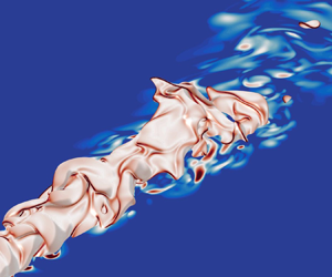
Figure 3 shows the dilatation field  $\boldsymbol {\nabla } \boldsymbol {\cdot } \boldsymbol {u}$ of the BFER case, both with and without the inlet sponge. The dilatation represents the divergence of the flow velocity field, which has been shown to be directly related to the pressure in the far field through the following equation (Colonius, Lele & Moin Reference Colonius, Lele and Moin1997):
 \begin{equation} \frac{\partial p}{\partial t} + \rho_{\infty} c_{\infty} \boldsymbol{\nabla} \boldsymbol{\cdot} \boldsymbol{u} = 0, \end{equation}
Figure 3. Dilatation field of the BFER case without the inlet sponge layer (a) and with the inlet sponge layer (b).
Figure 3 shows that the inlet sponge has significantly reduced the noise generated from the injection of turbulence. In addition, the flow field statistics downstream of the inlet were not significantly affected by the presence of the sponge layer at the inlet.
3. Theoretical framework
3.1. Relationship between heat release rate and combustion noise
The heat release rate term appearing in the governing equation for the sensible enthalpy is used in the following (Poinsot & Veynante Reference Poinsot and Veynante2005, p. 18):
 \begin{equation} \dot{Q} ={-} \sum_{\alpha=1}^{N_s} {\rm \Delta} h_{f\alpha}^0 {\hat{\dot \omega}}_\alpha ={-} \sum_{\alpha=1}^{N_s} \sum_{j=1}^{N_r} {\rm \Delta} h_{f\alpha}^0 (\nu_{j\alpha}^{\prime\prime} - \nu_{j\alpha}^{\prime}) \dot{\omega}_j. \end{equation}
Here  $N_r$ represents the number of reactions in the chemical mechanism,
  $\nu _{j\alpha }'$ and
  $\nu _{j\alpha }''$ are respectively the reactant-side and product-side stoichiometric coefficients associated to species
  $\alpha$ and reaction
  $j$,
$j$,  ${\rm \Delta} h_{f\alpha }^0$ is the enthalpy of formation of species
  $\alpha$ at standard conditions,
  $\dot {\omega }_j$ is the reaction rate of reaction
  $j$ and
  ${\hat{\dot \omega}}_\alpha$ is the production rate of species
  $\alpha$. The acoustic source term in (1.1) can therefore be written as
 \begin{equation} \frac{\partial \dot{Q}}{\partial t} = \sum_{j=1}^{N_r} \frac{\partial \dot{Q}_j}{\partial t} ={-} \sum_{\alpha=1}^{N_s} \sum_{j=1}^{N_r} (\nu_{j\alpha}^{\prime\prime} - \nu_{j\alpha}^{\prime}) {\rm \Delta} h_{f\alpha}^0 \frac{\partial \dot{\omega}_j}{\partial t}, \end{equation}
where  $\dot {Q}_j$ denotes the heat release rate associated with reaction
  $j$. Equation (3.2) explicitly shows that the rate of change of reaction rates
  $\partial \dot {\omega }_j / \partial t$ has a direct impact on
  $\partial \dot {Q} / \partial t$ and, therefore, on the generated sound. The term
  $\partial \dot {Q} / \partial t$ can be related to the fluctuations of the heat release rate
  $\dot {Q}'$ by a time scale
  $\tau _1$ such that the following relationship for the acoustic power can be established:
 \begin{equation} {\overline{p'^2}} \propto \overline{ \left( \int \partial \dot{Q} / \partial t \,\textrm{d} V \right)^2} = \frac{1}{\tau_1^2} \overline{\left( \int \dot{Q}' \,\textrm{d} V \right)^{2}}. \end{equation}
Here the overline denotes temporal averaging. Equation (3.3) will be used in § 4.3 to examine the impact of heat release rate fluctuations on the generated sound. A similar approach was used by Swaminathan et al. (Reference Swaminathan, Xu, Dowling and Balachandran2011) to model the overall acoustic sound pressure level (OASPL) of turbulent premixed flames. Following a reasoning analogous to their study, a further decomposition of  $\dot {Q}' = \dot {Q} - \bar {\dot {Q}}$ shows that
  $\partial \dot {Q} / \partial t$ can also be related to the heat release rate using a different time scale
  $\tau _2$,
 \begin{equation} {\overline{p'^2}} \propto \overline{ \left( \int \partial \dot{Q} / \partial t\,\textrm{d} V \right)^2} = \frac{1}{\tau_2^2} \overline{\left( \int \dot{Q} \,\textrm{d} V \right)^{2}}. \end{equation}
 Note that the time scales  $\tau _1$ and
  $\tau _2$ have different physical interpretations. While
  $\tau _1$ indicates how effectively fluctuations of the heat release rate produce sound,
  $\tau _2$ shows how effectively heat is converted to sound. By extending (3.4) to individual reactions using a time scale
  $\tau _{2,j}$, the contribution of reaction
  $j$ to the generated sound can be estimated as
 \begin{equation} \overline{p'^2} \propto \sum_{j=1}^{N_r} \left[ \frac{1}{\tau_{2,j}^2} \overline{\left( \int \dot{Q}_j \,\textrm{d} V \right)^2} + \sum_{k=1,\ k \neq j}^{N_r} \overline{ \int \frac{\partial \dot{Q}_j}{\partial t} \,\textrm{d} V \int \frac{\partial \dot{Q}_k}{\partial t} \textrm{d} V} \right]. \end{equation}
 The first term in the square brackets denotes the contribution of reaction  $j$ only while the second term represents the cross-contribution of reactions
  $j$ and
  $k$. Equations (3.4) and (3.5) will be used in § 4.3 to analyse the relative contribution of different reactions to combustion noise.
3.2. Relationship between flame stretch and combustion noise
According to Tam et al. (Reference Tam, Bake, Hultgren and Poinsot2019), a mechanistic theory relating flame front dynamics to sound generation can shed light on the sources of combustion noise. Such a framework is provided by (1.3). The flame stretch, noted as  $\kappa$, represents the local change of the flame surface area,
 \begin{equation} \kappa = \frac{1}{\delta A} \frac{\textrm{d}(\delta A)}{\textrm{d} t}, \end{equation}
where  $\delta A$ represents an infinitesimal portion of the flame surface. The overall
  $\textrm {d} A/\textrm {d} t$ can therefore be written as
 \begin{equation} \frac{\textrm{d} A}{\textrm{d} t} = \frac{\textrm{d}}{\textrm{d} t} \int_{A} \delta A =\int_{A} \frac{\textrm{d}(\delta A)}{\textrm{d} t} = \int_{A} \kappa \delta A, \end{equation}
so that (1.3) can be expressed as
 \begin{equation} p'(r_s,t)= \frac{\rho_{\infty} S_L}{4{\rm \pi} r_s} \left( \frac{\rho_u}{\rho_b} - 1 \right) \left[ \int_{A} \kappa \delta A \right]_{t-r_s/c_{\infty}}. \end{equation}
 The flame stretch rate can be expressed as the sum of a dilatation term ( $\kappa _{D}$), a normal strain rate term (
 $\kappa _N$) and a curvature term (
 $\kappa _C$) (Matalon Reference Matalon1983; Candel & Poinsot Reference Candel and Poinsot1990), i.e.
 \begin{equation} \kappa= \kappa_D + \kappa_N + \kappa_C = \frac{\partial u_i}{\partial x_i} - n_i n_j \frac{\partial u_i}{\partial x_j} + S_d \frac{\partial n_i}{\partial x_i}, \end{equation}
where  $S_d$ is the local flame displacement speed and
  $\boldsymbol {n}$ is the unit flame normal vector pointing towards the unburnt mixture. The positive values of
  $\kappa$ represent flame surface generation while negative values indicate flame surface destruction. The term
  $\partial n_i / \partial x_i$ in (3.9) represents the flame surface curvature. This term will be negative when the flame is curved towards the unburnt gases and positive when curved towards the burnt gases. Markstein (Reference Markstein1964) developed what is known as Markstein linear theory, relating the flame displacement speed to flame curvature as
 \begin{equation} \frac{S_d}{S_L} = 1 - l_M \boldsymbol{\nabla} \boldsymbol{\cdot} \boldsymbol{n}, \end{equation}
where the proportionality constant,  $l_M$, is known as the Markstein length. Equation (3.10) is a simple framework that has been extensively examined in the literature. For instance, Peters et al. (Reference Peters, Terhoeven, Chen and Echekki1998) and Peters (Reference Peters1999) also derived a linear relationship between
  $S_d$ and curvature to model flames in the thin-reaction zone with the G-equation, and verified the validity of the formulation using DNS of two-dimensional (2-D) unsteady methane/air flames. Recently, Dave & Chaudhuri (Reference Dave and Chaudhuri2020) studied the behaviour of
  $S_d$ in a turbulent hydrogen/air flame featuring flame annihilation events, which are characterised by large negative curvatures and large stretch. They showed that a linear relationship between
  $S_d$ and curvature can be used for these annihilation events. In addition, Trivedi et al. (Reference Trivedi, Griffiths, Kolla, Chen and Cant2019) used Morse theory to show that
  $S_d$ is linearly dependent on curvature during pocket formation.
In this framework of large curvature values,  $\kappa _D$ and
  $\kappa _N$ become negligible so that
  $\kappa \simeq \kappa _C$. Under the assumption that Markstein linear theory holds, (3.8) and (3.10) can be combined to express the far field noise as
 \begin{equation} p'(r_s,t)= \frac{\rho_{\infty} S_L^2}{4{\rm \pi} r_s} \left( \frac{\rho_u}{\rho_b} - 1 \right) \left[\int_{A} \boldsymbol{\nabla} \boldsymbol{\cdot} \boldsymbol{n} \left( 1 - l_M \boldsymbol{\nabla} \boldsymbol{\cdot} \boldsymbol{n} \right) \delta A \right]_{t-r_s/c_{\infty}}. \end{equation}
 Equation (3.11) shows that the pressure fluctuations have a strong dependence to the flame surface curvature. Note that the  $S_L^2$ acoustic dependence for spherically symmetric annihilation events demonstrated by Talei, Brear & Hawkes (Reference Talei, Brear and Hawkes2011) is retrieved here. Equation (3.11) will be used in § 4.4 to relate the flame dynamics to combustion noise.
4. Results and discussion
4.1. Flame/turbulence interaction
The progress variable  $C$ is defined based on the
  $\text {O}_2$ mass fraction, as commonly defined in DNS studies of premixed methane/air flames (Sankaran et al. Reference Sankaran, Hawkes, Chen, Lu and Law2007; Vreman et al. Reference Vreman, Van Oijen, De Goey and Bastiaans2009; Thornber et al. Reference Thornber, Bilger, Masri and Hawkes2011; Wang, Hawkes & Chen Reference Wang, Hawkes and Chen2016),
 \begin{equation} C = \frac{Y_{\text{O}_2} - Y_{\text{O}_2,u}}{Y_{\text{O}_2,b} - Y_{\text{O}_2,u}}. \end{equation}
 The progress variable is therefore zero in the unburnt mixture and unity in the fully burnt region. The unit flame normal vector  $\boldsymbol {n}$ is defined as
  $\boldsymbol {n} = - \boldsymbol {\nabla } C / | \boldsymbol {\nabla } C |$ and the local curvature as
  $\boldsymbol {\nabla } \boldsymbol {\cdot } \boldsymbol {n}$. The instantaneous flame surface is defined based on the progress variable isosurface corresponding to the location of the maximum heat release rate in an unstrained 1-D laminar flame under the same conditions as the turbulent flames. This progress variable equals to
  $0.82$ and
  $0.62$ for the BFER and COFFEE cases, respectively.
The instantaneous flame surface of the two cases, coloured with the absolute value of the flame surface curvature, are shown in figure 4. As pointed out by the ellipses in the left panels, both flames have similar features close to the inlet. This similarity is expected as the boundary conditions at the inlet are the same. However, the flame surfaces become increasingly different further downstream, showing that the kinetics impact the flame dynamics. The COFFEE flame appears more wrinkled and features more detached pockets of unburnt mixture. As discussed in previous studies (Rajaram & Lieuwen Reference Rajaram and Lieuwen2009; Haghiri et al. Reference Haghiri, Talei, Brear and Hawkes2018), most of the acoustic sources are concentrated around the flame tip. Therefore, the difference between the two flames in that region can lead to different far field noise, as it will be discussed in § 4.4.

Figure 4. Instantaneous isosurfaces of progress variable  $C=0.82$ and
  $C=0.62$ for the BFER and COFFEE flames, respectively, coloured by the flame curvature magnitude.
In cylindrical coordinates the flame surface normal is written as  $\boldsymbol {n} = [n_x, n_r, n_{\theta }]$, where
  $n_x$,
  $n_r$ and
  $n_{\theta }$ represent the flame normal components in the streamwise, radial and azimuthal directions, respectively. To investigate the orientation of the flame surface, the probability density functions (PDFs) of
  $\boldsymbol {n}$ are shown in the left panels of figure 5. Close to the inlet (at
  $x/D=2$), the flames have the same orientation, consistent with figure 4. The preferred value for the radial orientation is
  $-1$, while the preferred value for the streamwise and azimuthal components is close to 0, meaning that the orientation is similar to that of the cylindrical laminar flame imposed at the inlet. Further downstream, at
  $x/D=10$, the radial and azimuthal PDFs are still similar. These distributions are very broad, with no preferred orientation and, therefore, feature a PDF value around 0.5. The streamwise PDFs are slightly different between the two cases in the upper half of the flame. The maximum PDF value occurs at
  $n_x=0$ for the BFER case, meaning that the flame will tend to be parallel to the streamwise jet centreline. On the other hand, the COFFEE flame has an orientation with less preference to any direction, consistent with the higher level of wrinkling observed earlier.

Figure 5. Probability density functions of (i) the flame normal  $\boldsymbol {n}$ components and (ii) the flame normal strain rate alignment
  $| \boldsymbol {n} \cdot \boldsymbol {e}_i |$ for the BFER (solid lines) and COFFEE (hollow markers) cases, at streamwise locations
  $x/D=2$ (a,b) and
  $x/D=10$ (c,d).
We now analyse flame/turbulence interaction to further examine and explain the differences between the two cases. The right panels in figure 5 show the PDFs related to the alignment between the flame normal and the strain rate eigenvectors  $\boldsymbol {e}_i$, which is characterised by the absolute value of the cosine angle between the vectors, i.e.
  $| \boldsymbol {n} \cdot \boldsymbol {e}_i |$. The eigenvectors
  $\boldsymbol {e}_1$ and
  $\boldsymbol {e}_3$ represent the most extensive and most compressive strain rates, respectively. The distributions show that the flames tend to align preferentially with
  $\boldsymbol {e}_3$ at downstream locations, consistent with the results of Ma, Talei & Sandberg (Reference Ma, Talei and Sandberg2020) for a similar Karlovitz number flame. Additionally, Baum et al. (Reference Baum, Poinsot, Haworth and Darabiha1994) reported a preferential alignment between
  $\boldsymbol {n}$ and
  $\boldsymbol {e}_3$ regardless of whether reduced or complex chemistry was used. The similarity between the BFER and COFFEE PDFs confirms this, implying that the flame-flow alignment is not dependent on the chemical modelling.
Figure 6(a) shows the instantaneous swirling strength  $\lambda _{c,i}$ and the flame surface at the central XY plane for both cases. Animations are provided as supplementary material available at https://doi.org/10.1017/jfm.2020.1184. The swirling strength is the imaginary part of the complex eigenvalues of the velocity gradient tensor (Zhou et al. Reference Zhou, Adrian, Balachandar and Kendall1999). The swirling strength is commonly used to identify vortical structures and has the advantage of being insensitive to the mean shear stress, contrary to vorticity. As expected, the vortical structures are very similar close to the inlet. The flame front tends to wrap around the vortices in the shear layer, creating typical flame cusps, as those seen around
  $x/D=2$. In the BFER case the vortices present in the shear layer decay more rapidly with increasing streamwise location compared with the COFFEE case, where strong swirling motions are still found around
  $x/D=6$ both in the unburnt and burnt gas regions. It indicates that chemical modelling can have an impact on the turbulence, even for flames with Karlovitz numbers which are an order of magnitude larger than unity.

Figure 6. (a) Instantaneous swirling strength  $\lambda _{c,i}$ and flame surface (white line) on the central
  $XY$ plane for the BFER and COFFEE cases. (b) Detailed view picturing the temporal evolution of a vortex/flame interaction in the COFFEE case.
Furthermore, a detailed inspection of several snapshots of vortex/flame interactions reveals that the vortices still deform the flame front in the upper-half of the COFFEE flame. In the panels displayed in figure 6(b), representing the COFFEE case, the vortex of interest (highlighted by the red arrow) stretches the flame, leading to a highly curved flame which eventually causes flame annihilation. This shows that the different flow dynamics in the unburnt region lead to different flame dynamics around the flame tip.
To further quantify the impact of chemical modelling on the flow field, the temporal mean of the turbulent kinetic energy (TKE) in the unburnt mixture (noted  $\overline {\text {TKE}}_u$) at the jet centreline is shown in figure 7. This quantity was obtained by conditioning the computation of the TKE to values of the progress variable lower than a threshold
  $C^+ = 0.05$ as
 \begin{equation} \text{TKE}_u = \tfrac{1}{2} \left( u_{i,u}'\right)^2 = \tfrac{1}{2} \left( u_i \mid_{C < C^+} - \overline{u_i \mid_{C < C^+}} \right)^2,\end{equation}
where  $u_{i,u}'$ denotes the
  $u_i$ r.m.s., conditioned in the unburnt region. For a point in the flame brush oscillating between unburnt and burnt gases, the velocity jump across the flame front leads to large TKE values, which are not representative of the turbulence level in the flow (Poinsot & Veynante Reference Poinsot and Veynante2005, p. 186–187). The conditioning used in (4.2) removes these effects when computing the velocity fluctuations (Shepherd, Moss & Bray Reference Shepherd, Moss and Bray1982; Cheng Reference Cheng1984).

Figure 7. Temporal mean of the TKE in the unburnt gases at the centreline.
Figure 7 shows that using different chemical mechanisms leads to very different  $\overline {\text {TKE}}_u$ in the region
  $4 < x/D < 8$, where the flow is more turbulent in the COFFEE flame. It is worth noting that the impact of flame on turbulence in the unburnt region has been reported in the literature (Furukawa et al. Reference Furukawa, Noguchi, Hirano and Williams2002; Steinberg, Driscoll & Ceccio Reference Steinberg, Driscoll and Ceccio2008). As it will be shown in § 4.3, the BFER case features a significantly higher heat release rate peak, which will increase the magnitude of the viscous dissipation term and the mean dilatation term in the TKE budget equation (Zhang & Rutland Reference Zhang and Rutland1995). The higher amplitude of these sink terms is expected to dampen turbulence more strongly.
The flame structure is another feature that is affected by turbulence. The surface density function  $| \boldsymbol {\nabla } C |$, which is representative of the inverse of the local flame thickness, can be used to assess how turbulence impacts the flame structure. Figure 8 shows the conditionally averaged
  $| \boldsymbol {\nabla } C |$ on
  $C$ for both cases, at several streamwise locations. The results from the unstrained laminar flame imposed at the inlet are also shown by the dashed lines. In the BFER case the flame becomes initially slightly thinner before thickening further downstream. However, the overall flame structure remains close to that of the laminar flame. With the COFFEE mechanism, a significant thickening occurs in the preheat region (
 $0.2 < C < 0.6$) for
  $x/D>5$. This result is expected for a flame in the thin-reaction zone and matches with the results from Sankaran et al. (Reference Sankaran, Hawkes, Chen, Lu and Law2007) for a preheated, lean, turbulent methane/air slot flame with a skeletal quasi-steady state chemistry mechanism. Note that the Karlovitz number is lower in the BFER case, due to the thinner flame obtained with this mechanism. It is therefore not surprising to observe a weaker impact of turbulence on the flame structure in this case. In addition, this result is consistent with previous studies pointing the reduced sensitivity of simple or semi-global chemistry flames to strain (Baum et al. Reference Baum, Poinsot, Haworth and Darabiha1994).

Figure 8. Surface density function  $| \boldsymbol {\nabla } C |$ conditionally averaged on the progress variable
  $C$ for different streamwise locations. The progress variable value corresponding to the flame surface is represented by the dotted red line and results from Sankaran et al. (Reference Sankaran, Hawkes, Chen, Lu and Law2007) are represented by hollow circles.
4.2. Combustion noise
To compare both flames in terms of acoustics, the pressure traces at  $[x,y,z]=[15D,8D,0D]$ are used since this point is reasonably far from both the inlet and the flame. A power spectral density estimate
  $S$ is obtained using Welch's method (Welch Reference Welch1967) with six Hanning windows and a 50 % overlap. The result is normalised and converted to the sound pressure level (SPL) spectra,
 \begin{equation} \text{SPL}(St) = 10 \log \left( \frac{S_{p'p'}}{S_0} \right), \end{equation}
where  $S_0$ is a reference power spectral density amplitude, taken as the maximum
  $S_{p'p'}$ value in the BFER case. The resulting SPL spectra are shown in figure 9, as a function of the Strouhal number, defined as
  $St=fD/\bar {u}_{in}$, where
  $f$ represents the frequency.

Figure 9. Pressure spectra at the location  $[x,y,z]=[15D,8D,0]$ for the BFER (solid line) and COFFEE (dashed line) cases.
The peak SPL values occur at  $St= 0.16$ and
  $St= 0.27$ for the BFER and COFFEE cases, respectively. The acoustic peak for the COFFEE case is 3 dB lower than that of the BFER case. The biggest differences, however, occur in the frequency range
  $1 < St < 5$, where the COFFEE spectrum typically has a 10 dB greater SPL.
The OASPL is defined as
 \begin{equation} \text{OASPL} = 10 \log \left( \int \frac{S_{p'p'}(\,f)}{S_0} \textrm{d} f \right) = 20 \log \left(\frac{p^{\prime}_{rms}}{p_0} \right),\end{equation}
where  $p_0$ represents a reference pressure level, and is 3.5 dB larger in the BFER case. This corresponds to approximately a 50 % difference in
  $p^{\prime}_{rms}$ and is illustrated by the different SPL at low frequencies, which contains most of the acoustic energy.
The assumption that  $\partial \dot {Q} / \partial t$ is the dominant source of noise is now examined. A posteriori pressure traces at the location
  $[x,y,z]=[15D,8D,0D]$ are computed from the acoustic source term
  $\partial \dot {Q} / \partial t$, using a discretised form of (1.1). A more detailed description of the method can be found in Brouzet et al. (Reference Brouzet, Haghiri, Talei and Brear2019). The DNS and a posteriori pressure traces and spectra are shown in figure 10. The pressure fluctuations from DNS and those generated by
  $\partial \dot {Q} / \partial t$ have a correlation coefficient above 0.8 for both cases. Considering the spectra reveals that
  $\partial \dot {Q} / \partial t$ is clearly the dominant source of noise up to
  $St=5$. The discrepancy observed for low SPL amplitudes at very high frequencies is believed to arise from the temporal interpolation of the acoustic source term
  $\partial \dot {Q} / \partial t$ at time
  $t - r_s/c_{\infty }$. Considering the importance of
  $\partial \dot {Q} / \partial t$ on the generated sound, the impact of chemical modelling on
  $\dot {Q}$ and
  $\partial \dot {Q} / \partial t$ is analysed in the next section.

Figure 10. (i) Pressure traces and (ii) pressure spectra at the location  $[x,y,z]=[15D,8D,0]$ directly extracted from the DNS (solid lines) and computed from
  $\partial \dot {Q} / \partial t$ with (1.1) (dashed lines) for the BFER (a,b) and COFFEE (c,d) cases.
4.3. Impact of chemical modelling on  $\dot {Q}$ and $\partial \dot {Q} / \partial t$


The time-averaged temperature fields of both cases are displayed in the left panels of figure 11. The slower post-flame reactions present in the skeletal COFFEE mechanism still release a significant amount of heat for  $x/D>L_{flame}$, resulting in a slow but gradual temperature increase in that region. As discussed in § 3.1, the acoustic power can be estimated using the r.m.s. of the volume integrated heat release rate fluctuations (3.3). Figure 11(b) shows that most of the heat release rate fluctuations arise from the flame brush. Indeed, inspection of the COFFEE case reveals that the heat release rate fluctuations in the post-flame region are typically one to two orders of magnitude lower than in the flame brush, suggesting that the post-flame region has negligible contributions to the generated sound.

Figure 11. (a) Temporally averaged temperature and (b) r.m.s. of the heat release rate fluctuations on the central XY plane.
The time scale  $\tau _1$ that relates
  $\dot {Q}'$ to the acoustic source term
  $\partial \dot {Q} / \partial t$ was computed using (3.3), and was equal to 5.1 and 5.2 time units for the BFER and COFFEE cases, respectively. This means that the difference in the acoustic power can be directly estimated by comparing the integrated fluctuations of the heat release rate. The r.m.s. value of the volume integrated
  $\dot {Q}'$ is larger by 60 % in the BFER case, consistent with the OASPL difference previously observed in § 4.2. In addition, the time scale
  $\tau _2$ relating
  $\dot {Q}$ to
  $\partial \dot {Q} / \partial t$, computed with (3.4), is significantly larger in the COFFEE case, meaning that the COFFEE mechanism will produce smaller fluctuations of the heat release rate. The remainder of this section aims at exploring the reasons leading to this
  $\dot {Q}'$ discrepancy.
Equation (3.5) is now used to examine the contribution of individual reactions to the overall generated sound. Figure 12 shows how efficient a given reaction is at converting heat into sound. The dashed lines show the following relationship using different values of  $\tau _2$:
 \begin{equation} \overline{ \left( \int \partial \dot{Q} / \partial t \,\textrm{d} V \right)^2} = \frac{1}{\tau_2^2} \overline{\left( \int \dot{Q} \,\textrm{d} V \right)^{2}}. \end{equation}
Figure 12. Scatter plot of  $\overline {( \int \dot {Q}_j \,\textrm {d} V )^2}$ and
  $\overline { ( \int \partial \dot {Q}_j / \partial t \,\textrm {d} V )^2}$ for the reactions in the BFER and COFFEE mechanisms. The dashed lines represent constant
  $\tau _2$ values. The dotted–dashed line represents the time scale
  $\tau _{flame}=L_{flame}/U_{bulk} \approx 50$ time units.
Since this figure is shown using a log-log scale, all dashed lines have a slope of 1. The higher the line is, the faster the reaction is, meaning that it is more efficient at converting heat into sound. The dotted–dashed line represents the flame time scale  $\tau _{flame}$ defined as the ratio of the mean flame length to the inlet bulk velocity
  $L_{flame}/U_{bulk} \approx 50$ time units. This time scale therefore represents the average time taken by a reactant molecule to reach the flame tip, where it will be consumed. It is not surprising to note that
  $\tau _{flame}$ features a value very close to the time scale
  $\tau _{2,j}$ of the dominant and most efficient reactions.
In addition, it is observed that the two reactions in the BFER mechanism feature a similar time scale  $\tau _{2,j}$, close to
  $\tau _{flame}$. However, a wide range of time scales is found in the COFFEE mechanism, spreading from 40 time units (
 $\textrm {HCO}+\textrm {O}\Leftrightarrow \textrm {CO}+\textrm {OH}$) to 450 time units (
 $\text {HO}_2 +\textrm {CO}\Leftrightarrow \text {CO}_2+\textrm {OH}$) and illustrating the variety of reactions that are modelled in this mechanism. These acoustically less efficient reactions explain the higher overall
  $\tau _2$ time scale of the COFFEE flame.
Further examination of the results presented in figure 12 showed that the acoustically dominant reaction for each mechanism was the most exothermic reaction,
 \begin{gather} \text{CH}_4 + 1.5\text{O}_2 \Rightarrow \text{CO}+2\text{H}_2 \text{O} \quad (\text{BFER}), \end{gather}
 \begin{gather}\text{CH}_3 + \text{O} \Leftrightarrow \text{CH}_2\text{O}+\text{H} \quad (\text{COFFEE}). \end{gather}
 Using (3.2), the contribution of every reaction to the overall  $\partial \dot {Q} / \partial t$ is computed. Figure 13 demonstrates the contribution of the acoustically dominant reaction to the total
  $\partial \dot {Q} / \partial t$, which accounted for 70 % of the total
  $\int \partial \dot {Q} / \partial t \,\textrm {d} V$ r.m.s. The high correlation between the two terms is also evident. A 3 dB difference is observed at the lowest frequencies while there are no significant differences for
  $St>1$.

Figure 13. (i) Temporal evolution and (ii) corresponding power spectral densities of the volume integral of  $\partial \dot {Q} / \partial t$ for all the reactions (solid lines) and the most exothermic reaction (dashed lines) in the BFER (a,b) and COFFEE (c,d) cases.
Figure 14 compares the heat release rate profiles of the most exothermic reactions of both mechanisms, in a 1-D freely propagating laminar flame. The most exothermic reaction has by far the largest contribution to the overall heat release rate compared with other reactions. The heat release rate peak of the dominant reaction, noted  $\dot {Q}_{d,max}$, is approximately 65 % of the overall heat release rate peak
  $\dot {Q}_{max}$, for both mechanisms. The ratio
  $\dot {Q}_{d,max}/\dot {Q}_{max}$ has a similar value to the ratio
 \begin{equation} {\int \frac{\partial \dot{Q}_d}{\partial t }\textrm{d} V}/{\int \frac{ \partial \dot{Q} }{\partial t} \textrm{d} V} \approx 0.70, \end{equation}
in the turbulent cases. This corroborates a scaling by Strahle (Reference Strahle1985), who argued that  $p' \propto \dot {Q}_{max}$. A higher
  $\dot {Q}_{max}$ obtained with the BFER mechanism is consistent with the larger fluctuations of the heat release rate for this case, observed in figure 11. This, in turn, leads to the OASPL discrepancy previously noted. It is therefore essential for a chemical mechanism to accurately model the heat release rate profile and its peak for a correct prediction of the overall acoustic power.

Figure 14. Total heat release rate (solid black line) and heat release rate of the most exothermic reactions for a 1-D freely propagating flame using the BFER (a) and COFFEE (b) mechanisms. The peaks of the total heat release rate and the most exothermic reaction are denoted by  $\dot {Q}_{max}$ and
  $\dot {Q}_{d,max}$, respectively.
4.4. Impact of stretch on combustion noise
The preceding section showed the importance of the heat release rate profile in determining the overall sound amplitude. We now consider flame/turbulence interaction in order to explain the observed differences at high frequencies in the acoustic spectra (figure 9). We first analyse the flame stretch and the stretch terms displayed in (3.9). Then, we relate stretch to combustion noise using the theory presented in § 3.2.
The PDFs of the different stretch terms are compared between the two cases in figure 15. The  $\kappa _N$ distribution is broader in the COFFEE flame and is skewed towards higher positive values. This shows that the flame with the more complex chemistry is more sensitive to the surrounding flow strain, in accordance with a result found by Baum et al. (Reference Baum, Poinsot, Haworth and Darabiha1994) for 2-D turbulent H
 $_2$ flames. The PDFs displayed in figure 15(b) show that
  $\kappa _D$ values are small compared with
  $\kappa _N$. Considering the scaling used in the literature for this term (Chakraborty & Swaminathan Reference Chakraborty and Swaminathan2007; Wang et al. Reference Wang, Hawkes and Chen2016),
 \begin{equation} \kappa_D \simeq \frac{{\rm \Delta} T}{T_u} \frac{S_L}{\delta_{th}}, \end{equation}
the magnitude of  $\kappa _D$ is about
  $0.1$, which is consistent with the results presented here. Finally, the
  $\kappa _C$ PDFs reveal that the curvature term has a tendency towards negative values in both cases.

Figure 15. Probability density functions of the (a) normal strain rate, (b) dilatation and (c) curvature terms of the flame stretch rate (3.9).
To further examine the relationship between strain and curvature contributions to stretch, the following theoretical argument is used. In a statistically stationary flame, the condition  $\overline {\textrm {d} A/\textrm {d} t}=0$ translates into
 \begin{equation} \overline{\int_{A} \kappa_N \delta A} ={-} \overline{\int_{A} \kappa_C \delta A}, \end{equation}
where the dilatation term  $\kappa _D$ has been neglected. Equation (4.10) shows that higher positive
  $\kappa _N$ values must be balanced by lower negative
  $\kappa _C$ values. Indeed, the mean
  $\kappa _C$ is 50 % lower in the COFFEE case, consistent with a higher mean
  $\kappa _N$ for this case. This difference is the subject of a comprehensive analysis later in this section. Equation (4.10) illustrates the equilibrium between flame surface generation and destruction, which was exemplified in figure 6(b) where a heavily strained flamelet led to an annihilation event. It is therefore important to note that the discrepancy observed between the two cases in terms of flame wrinkling (in figure 4) is a consequence of the different flame response to the flow strain.
To establish under which conditions the normal strain rate and the curvature stretch terms are dominant, the joint PDFs are examined in figure 16. The white dashed line represents the conditionally averaged  $\kappa$ terms on the total stretch. For positive stretch values, a strong correlation is observed between
  $\kappa _N$ and
  $\kappa$ (a,b), indicating that flame straining in the normal direction to the flame front is the dominant mechanism for generation of flame surface area. On the other hand,
  $\kappa _N$ values smaller than
  $-$0.5 are rare, indicating that strain does not significantly contribute to the destruction of the flame surface area. The joint PDF of the dilatation and global stretch (c,d) confirms that
  $\kappa _D$ is negligible and has no correlation with
  $\kappa$.

Figure 16. Joint PDFs of the flame stretch  $\kappa$ with its components
  $\kappa _N$ (a,b),
  $\kappa _D$ (c,d) and
  $\kappa _C$ (e,f ) for the BFER (a,c,e) and COFFEE (b,d,f ) cases.
The bottom row in figure 16 shows that  $\kappa _C$ is dominant for values lower than
  $-$0.5. This is even clearer showing the full range of
  $\kappa$ and
  $\kappa _C$ in figure 17, which reveals an excellent correlation between these two quantities for highly negative values of stretch. To summarise, the normal strain and the curvature terms are dominant for
  $\kappa >0$ and
  $\kappa < -0.5$, respectively. However, neither
  $\kappa _N$ or
  $\kappa _C$ are dominant for mildly negatively stretched flamelets (
 $-0.5<\kappa <0$).

Figure 17. Expanded view of the joint PDFs of the flame stretch  $\kappa$ with
  $\kappa _C$ for the BFER (a) and COFFEE (b) cases. The dashed boxes represent the extent of the views shown in figure 16.
As shown in our previous studies, destruction of the flame surface area plays a major role in terms of the generated sound, in particular for high frequencies (Haghiri et al. Reference Haghiri, Talei, Brear and Hawkes2018; Brouzet et al. Reference Brouzet, Haghiri, Talei and Brear2019). The focus is therefore placed on negative stretch values, when  $\kappa _C$ is dominant. To compare in greater detail the stretch PDFs between the BFER and COFFEE cases, logarithmic scales are used in figure 18(a). While the distributions are similar for low stretch values, they become increasingly different as the magnitude of stretch increases. In the range
  $1 < - \kappa < 20$, the stretch PDF of the COFFEE flame has an average value more than twice as high as that of the BFER flame.

Figure 18. Probability density functions of the (a) flame stretch  $\kappa$, (b) normalised flame displacement speed
  $S_d/S_L$ and (c) curvature
  $\boldsymbol {\nabla } \boldsymbol {\cdot } \boldsymbol {n}$.
According to (3.9), negative  $\kappa _C$ are associated with negative values of curvature, i.e. flame curved towards the unburnt gas (assuming that the flame displacement speed remains positive). The PDFs of positive
  $S_d$ and negative
  $\boldsymbol {\nabla } \boldsymbol {\cdot } \boldsymbol {n}$ values are examined in figures 18(b) and 18(c) to understand how they affect the stretch statistics. When plotted on logarithmic scales, there is an insignificant difference between the flame displacement speed PDFs for
  $S_d/S_L>10$, indicating that the higher occurrence of highly negative stretch in the COFFEE case is not due to large values of
  $S_d$. Inspection of the curvature PDFs shows however that highly curved flame regions (
 $- \boldsymbol {\nabla } \boldsymbol {\cdot } \boldsymbol {n} > 30$) are more present in the COFFEE case, confirming the qualitative observation from figure 4 that this flame is more wrinkled. To illustrate the highly curved surfaces, figure 19 shows a zoomed view of the COFFEE flame, coloured by the local value of curvature. Both elongated cusp regions and annihilation events, highlighted by the black and red circles, respectively, are found to feature highly curved surfaces.

Figure 19. An instantaneous flame surface in the COFFEE case coloured with the flame curvature, showing elongated cusps (black ellipse) and flame annihilation (red circle).
Up to this point, the flame with a more complex chemistry was found to be more stretched and to feature more highly curved surfaces. As shown by (3.8) and (3.11), this should lead to different acoustic outputs between the two flames. To asses this, we first verify the validity of Markstein linear theory (3.10), which was used to derive (3.11). Figure 20 shows the joint PDFs of curvature and flame displacement speed for the two flames. The least-squares linear fit, considering  $S_d/S_L>0$ and
  $\boldsymbol {\nabla } \boldsymbol {\cdot }\boldsymbol {n} < 0$, is represented by the solid red line. Even though Markstein theory was developed for low curvature values, there is a strong dependency between
  $S_d$ and
  $\boldsymbol {\nabla } \boldsymbol {\cdot } \boldsymbol {n}$ for a large range of curvatures, as also found by other studies (see § 3.2). The correlation coefficient between the two variables is 0.85, for both cases. The Markstein length extracted from the least-squares fit equals
  $l_M=0.435$ and
  $l_M=0.306$ for the BFER and COFFEE flames, respectively.

Figure 20. Joint PDFs of curvature and flame displacement speed for the BFER (a) and COFFEE (b) cases. The solid red lines represent the least-squares linear fit.
A scaling proposed by Strahle (Reference Strahle1971) is now used to investigate the impact of curvature on the generated sound. He argued that the characteristic time scale  $\tau _c$ associated with the flame motion is equal to the time of passage of a fluid element through the turbulent flame zone, i.e.
  $\tau _c \approx \delta _c/S_d$, where
  $\delta _c$ represents a characteristic flame thickness. Using this argument, a characteristic acoustic frequency
  $f_c$ is defined based on the local flame displacement speed so that
  $f_c \approx S_d/\delta _c$. As this scaling is used here to relate the flame motion to the generated sound, the characteristic flame thickness
  $\delta _c$ should be relevant to sound generation. The acoustically dominant reactions were therefore used to obtain
  $\delta _c$, which is defined as the full width at tenth maximum of the dominant reaction heat release rate, leading to values of
  $\delta _c=0.127$ and
  $\delta _c=0.099$ for the BFER and COFFEE cases, respectively.
Using Markstein linear theory to relate  $S_d$ to
  $\boldsymbol {\nabla } \boldsymbol {\cdot }\boldsymbol {n}$, the following characteristic Strouhal number is then defined:
 \begin{equation} St_c = \frac{f_c D}{M} = \frac{S_d D}{\delta_c M} = \frac{(1-l_M \boldsymbol{\nabla} \boldsymbol{\cdot} \boldsymbol{n}) S_L D}{\delta_c M}. \end{equation}
 The PDF of curvature is established by considering a number of bins in the curvature space. According to (4.11), each bin has a unique characteristic Strouhal number. It is recalled that for large negative values of curvature, (3.11) shows that  $p'$ is a function of curvature only. One can therefore conclude that the pressure fluctuations spectrum in the far field must correlate with the curvature PDF. Assuming that the acoustic amplitude at the characteristic frequency
  $St_c$ is proportional to the number of occurrences, the curvature PDF is converted to spectral space using (4.11).
Figure 21 shows the SPL spectra computed from the DNS  $p'$ (black lines) and the PDFs of
  $\boldsymbol {\nabla } \boldsymbol {\cdot } \boldsymbol {n}$ (red lines) which were converted to decibels by showing
  $20 \log _{10}(\text {PDF})$. The estimation from the curvature PDF shows a behaviour similar to the SPL spectra in the range
  $0.5 < St < 5$, retrieving the discrepancy between the two spectra at high frequencies. The mean difference between the BFER and COFFEE
  $20\log _{10}(\text {PDF})$ curves is 12 dB in the range
  $1 < St < 5$, which is in accordance with the mean
  $p'$ SPL difference in that range. The under-estimation for
  $St > 5$ and over-estimation for
  $St<0.5$ are believed to arise, respectively, from the Markstein linear theory and the
  $\kappa \approx \kappa _C$ assumptions not to be valid anymore.

Figure 21. Sound pressure level spectra from DNS (black) and estimated from the flame curvature PDF (red) for the BFER (solid lines) and COFFEE (dashed lines) cases.
This modelling shows that the trend of the SPL acoustic spectrum in the high frequency range is proportional to the occurrence of highly curved flamelets and can be estimated using the curvature PDF. Furthermore, it shows that the discrepancy between the semi-global BFER mechanism and the more complex skeletal COFFEE chemistry arises from different flame dynamics and, more specifically, from more occurrences of highly curved flame surfaces in the latter case.
5. Conclusion
The impact of chemical modelling on the flame dynamics and sound generation by turbulent premixed methane/air jet flames was investigated using DNS. The semi-global BFER mechanism (Franzelli et al. Reference Franzelli, Riber, Gicquel and Poinsot2012) and the more complex skeletal COFFEE mechanism (Coffee Reference Coffee1984) were used to perform these simulations.
It was first observed that these two chemical mechanisms resulted in similar flame structures close to the jet inlet. However, the flame modelled with the COFFEE mechanism was more wrinkled at downstream locations. Furthermore, the swirling strength and the TKE in the unburnt gases were higher with the COFFEE mechanism. These different dynamics indicate that the two-way coupling between the flame and turbulence depends on the choice of chemical mechanism.
The flame modelled with the COFFEE mechanism was also observed to have a significantly lower total acoustic power even though this case radiated more sound at high frequencies. The former result was due to this flame's smaller fluctuations in heat release rate, resulting from differences in the heat release rate profile. In both cases, the time derivative of the heat release rate  $\partial \dot {Q} / \partial t$ was nonetheless the dominant acoustic noise source, as previous studies have shown, with the most exothermic reaction contributing to a substantial fraction of the generated sound.
The physical processes by which the COFFEE mechanism created greater acoustic content at high frequencies were then examined. Markstein's linear theory was first used to develop a model that related the acoustic spectrum to the PDF of the flame curvature. This demonstrated that this higher frequency acoustic content was the direct result of the COFFEE mechanism creating more wrinkled flame surfaces.
These results suggest that the accurate simulation of the noise emitted by turbulent premixed flames requires a chemical mechanism that ensures two main features. First, accurate modelling of the overall sound amplitude and the lower frequency acoustic spectra appears to require accurate modelling of the heat release rate profile in a 1-D sense. Second, accurate modelling of the acoustic spectrum at higher frequencies should first capture the flame/turbulence interaction. Whether a single, reduced order mechanism can address both priorities is not obvious, and will be considered further in future research.
Supplementary movies
Supplementary movies are available at https://doi.org/10.1017/jfm.2020.1184.
Funding
This work was supported by the Australian Research Council (ARC) [DE180100416] and the University of Melbourne through a Melbourne International Research Scholarship and a Melbourne International Fee Remission Scholarship. The research benefited from computational resources provided through the National Computational Merit Allocation Scheme and the Pawsey Energy and Resources Scheme, supported by the Australian Government. The computational facilities supporting this project included the Australian NCI National Facility and the Pawsey Supercomputing Centre.
Declaration of interests
The authors report no conflict of interest.
Appendix A. Chemical mechanisms
A.1. Semi-global BFER mechanism

A.2. Skeletal COFFEE mechanism


