1. Introduction
What makes a scientific model explanatory? This is a topic that has received considerable attention of late in the philosophy of science literature. It is intimately bound up with questions about the nature and role of idealizations, about the role of mathematics in empirical investigations, and about what counts as a scientific representation. In this article we argue that there is a class of explanatory models whose explanatory structure has been almost universally misunderstood by philosophers. These models are used to explain patterns of macroscopic behavior across systems that are heterogeneous at smaller scales. We call these models “minimal models,” and our goal is to provide some examples and an analysis of what actually does the explanatory work when such models are employed. Perhaps the remarkable feature of minimal models is that they are thoroughgoing caricatures of real systems. This fact raises the following question: How can a model that really looks nothing like any system it is supposed to “represent” play a role in allowing us to understand and explain the behavior of that system? We take the lack of similarity or representation quite seriously and argue that the existing philosophical literature looks in the wrong place to try and understand what makes these models explanatory, by only looking at the features they have in common with real systems. Instead, we will show that an explanatory story devoid of representation relations is required to understand how these models can be used to such great effect. In many cases, considerations of representational accuracy are inadequate to explain why so many diverse systems, including the model system, will display the same macroscale behavior. It is only once we have a fundamentally different kind of story about how these minimal models “latch onto the world” that we can see in virtue of what they are able to explain universal patterns across diverse real systems.Footnote 1 This alternative story also shows why those different/heterogeneous systems can be modeled by such minimal models, why the heterogeneous systems have certain very general features in common, and how those features are related to the macroscale behavior of those systems. We show how to provide an explanation of patterns that are realized by diverse systems and also demonstrate how a minimal model can be employed to understand the behavior of real systems.
Let us explicitly lay out the main argument of the article:
1. Most philosophical accounts claim that a model explains just when it has certain relevant features in common with actual systems and that having these features in common is exactly what does the explaining.
2. There are several cases in which a model explains a universal pattern, but simply citing those features the model has in common with real systems misidentifies what makes it explanatory.
3. Therefore, these models must be explanatory in virtue of some other connection with real-world systems.
We then argue that, in many cases, this alternative connection can only be understood by moving beyond the features represented within the model itself and by paying attention to a process of delimiting a universality class, by demonstrating that the details that distinguish the model system and various real systems are irrelevant. In these minimal model explanations, the key connection between the model and the diverse real-world systems is that they are in the same universality class.
In Section 2, we discuss a number of recent accounts of what makes a model explanatory that, despite their differences, can be grouped under the heading of “common features accounts.” These accounts all hold that some kind of accurate mirroring, or mapping, or representation relation between model and target is responsible for the explanatory success of the model. We then argue that these accounts fail to provide answers to several explanatory questions that are essential for understanding patterns displayed by distinct systems. Sections 3 and 4 present and analyze two examples of the use of minimal models to provide explanations—one from fluid mechanics and one from population biology. These examples are just two instances of a large class of minimal model explanations in science. We detail the models and show how they can be explanatory despite an almost complete lack of correspondence with any real fluid system or biological population.
2. Common Features Accounts
Many accounts of explanatory models claim that a model is explanatory because it has certain relevant features in common with the model’s target system(s). Indeed, several recent accounts of explanation, idealization, and the role of mathematics in scientific explanation involve claims to the effect that a model explains in virtue of “accurately representing,” “mirroring,” or “mapping onto” the relevant features of its target system(s). This section presents several of these accounts. We believe that none of these can adequately account for the explanatory role played by our examples of minimal models. These views may very well provide good reasons for why some models are explanatory, but as we argue below, their focus on representation misses what is explanatory when minimal models are employed. Our aim in this section is only to show that these accounts are all reasonably grouped under the heading “common features accounts” and that when applied to minimal models they will respond similarly to the second of the following two questions.
1. What accuracy conditions are required for the model to explain?
2. In virtue of what does the model explain?
We think these questions are importantly different. However, we think most philosophical accounts of explanatory models conflate them in the following sense. They answer the second by citing that the accuracy conditions noted in response to the first are met. Each account presented in this section implies that a model explains in virtue of meeting some accuracy conditions.Footnote 2
2.1. Mechanistic Models
Accuracy requirements are prominent in various accounts that claim that only mechanistic models explain (Craver Reference Craver2006; Kaplan Reference Kaplan2011; Kaplan and Craver Reference Kaplan and Craver2011). Mechanistic accounts typically place extremely strict accuracy conditions on explanatory models by requiring that the model accurately describe the actual causal mechanism(s) that produced the phenomenon. For example, Kaplan’s and Craver’s model-mechanism-mapping (3M) requirement claims:
(3M) A model of a target phenomenon explains that phenomenon to the extent that (a) the variables in the model correspond to identifiable components, activities, and organizational features of the target mechanism that produces, maintains, or underlies the phenomenon, and (b) the (perhaps mathematical) dependencies posited among these (perhaps mathematical) variables in the model correspond to causal relations among the components of the target mechanism. (Kaplan Reference Kaplan2011, 347)
The 3M requirement involves various kinds of “correspondence” between the model and the actual causal mechanisms that produced the explanandum.Footnote 3 Furthermore, on this account, a model explains simply in virtue of having these corresponding features in common with the actual mechanisms that produce the phenomenon. For example, Craver tells us that (how-actually) models possess explanatory force because they describe the “real components, activities, and organizational features of the mechanism that in fact produces the phenomenon” (Reference Craver2006, 361). Furthermore, as Kaplan tells us, the 3M requirement aligns with the assumption “that the more accurate and detailed the model is for a target system or phenomenon the better it explains that phenomenon” (Reference Kaplan2011, 347). So not only does veridical representation of the causal mechanism make a model explanatory, the more accurate and detailed that representation is, the more explanatory the model will be.
We think this view is mistaken for a number of reasons. First, it gives far too much weight to the accuracy requirements for explanatory models. Many models are explanatory even though they do not accurately describe the actual causal mechanisms that produced the phenomenon (Cartwright Reference Cartwright1983; Batterman Reference Batterman2002b, Reference Batterman2010; Woodward Reference Woodward2003; Rice Reference Rice2012). Second, this view mistakenly implies that more accurate detail concerning mechanisms is always better. However, there are several reasons why the explanation provided by a model might be improved by removing various details concerning causal mechanisms (Cartwright Reference Cartwright1983; Batterman Reference Batterman2002b, Reference Batterman2009, Reference Batterman2010; Rice Reference Rice2012, Reference Rice2013). For example, in many cases we want to explain patterns that range over systems whose mechanisms are extremely different. In such cases, a model that accurately represented any particular mechanism would fail to provide an adequate explanation.
2.2. Causal/Difference-Making Models
Another class of accounts of explanatory models offers less strict accuracy requirements. Here we include contemporary causal theories of explanation that allow an explanation to be improved by removing irrelevant causal factors from the model (Salmon Reference Salmon1984; Woodward Reference Woodward2003; Strevens Reference Strevens2004, Reference Strevens2009). Still, these causal theories maintain some version of the accuracy requirement in that they require an explanatory model to accurately represent (or describe) the relevant (or difference-making) causes that produce the phenomenon to be explained. As Michael Strevens asserts, “no causal account of explanation—certainly not the kairetic account—allows nonveridical models to explain” (Reference Strevens2009, 320). As with many causal accounts, for Strevens, in order to provide an explanation the model must accurately represent causal relationships between the features cited in the explanans and the explanandum. On Strevens’s account, a “standalone explanation of an event e is a causal model for e containing only difference-makers for e” (73). What makes this explanation causal is that “the derivation of e, mirrors a part of the causal process by which e was produced” (75).
More generally, for causal accounts of explanation, in order for a model to be explanatory it must provide an accurate representation of the relevant causal relationships (or causal processes) within the model’s target system(s). Typically, this is done by having the relationships in the model mirror, correspond to, or map onto causal relationships in the target system. On these accounts, the explanatory power of a model comes from its having these relevant causes in common with the model’s target system(s).
These accounts of causal explanation have also led to various claims about how idealized models can provide explanations (Elgin and Sober Reference Elgin and Sober2002; Strevens Reference Strevens2004, Reference Strevens2009; Potochnik Reference Potochnik2007; Weisberg Reference Weisberg2007, Reference Weisberg2013). These accounts of idealization allow for the misrepresentation of irrelevant causal factors by the explanatory model. However, having the causally relevant features in common with real systems continues to play the essential role in showing how idealized models can be explanatory.Footnote 4 On Michael Weisberg’s account, “minimalist idealization is the practice of constructing and studying theoretical models that include only the core causal factors which gave rise to the phenomenon” (Reference Weisberg2007, 642).Footnote 5 According to Weisberg, a minimalist model “accurately captures the core causal factors” since “the key to explanation is a special set of explanatorily privileged causal factors. Minimalist idealization is what isolates these causes and thus plays a crucial role for explanation” (643–45). Among others, Weisberg cites Strevens’s (Reference Strevens2009) account of idealization as an example of minimalist idealization. Strevens explains his account of idealized models as follows: “The content of an idealized model, then, can be divided into two parts. The first part contains the difference-makers for the explanatory target. … The second part is all idealization; its overt claims are false but its role is to point to parts of the actual world that do not make a difference to the explanatory target. The overlap between an idealized model and reality … is a stand-alone set of difference-makers for the target” (318). In other words, these idealized models provide an explanation by (i) accurately representing (or ‘overlapping’ with) the causal difference makers and (ii) using idealizations to indicate those causal factors that are irrelevant. More generally, idealized models are explanatory just when they share relevant causes with the real system(s) and make idealizing assumptions that misrepresent irrelevant causes.
Although these types of accounts provide an improvement over the 3M view, we feel they suffer from two main problems. First, these accounts require that all explanatory models provide an accurate description of the causes of the explanandum. However, if one looks at the explanations actually offered by scientists it is often the case that one finds no appeal to causes at all (Batterman Reference Batterman2010; Huneman Reference Huneman2010; Pincock Reference Pincock2012; Rice Reference Rice2012, Reference Rice2013).Footnote 6 Instead, many model explanations appeal to structural, mathematical, topological, or some other noncausal features of the system. Second, while these (causal/difference-making) accounts allow idealized models to explain, the only role idealizations play is to indicate what causes are irrelevant. Therefore, in some sense, the idealizations themselves do not play any role in the actual explanation. The goal is to show that the idealizations are in some sense harmless because they do not “get in the way” of the accurate representation of the causes that are relevant (Elgin and Sober Reference Elgin and Sober2002). We think this fails to adequately capture the positive contributions that many idealizations make within explanatory models. Indeed, as we argue below, a positive role played by idealizations is in demonstrating (or deriving) the fact that various details are irrelevant, instead of just using them to isolate difference makers only after we know what is irrelevant. But perhaps more importantly, we think these views mistakenly claim that the “real explanatory work” in these cases is done by the veridical representation of difference-making features within the model. In contrast, our discussion of minimal models in sections 3 and 4 is designed to show how highly idealized models can play explanatory roles despite near complete representational failure. Furthermore, the minimal representational success in these minimal models is not what is responsible for the models’ abilities to explain.
2.3. Pincock’s Proposals
Finally, on our view, some of what Christopher Pincock says in his recent book Mathematics and Scientific Representation allows us to situate his views with the others under the common features umbrella. For example, Pincock argues that “we can distinguish at least three ways in which mathematics can contribute to the explanatory power of a scientific explanation. … These are by (i) tracking causes, (ii) isolating recurring features of a phenomenon, and (iii) connecting different phenomena using mathematical analogies” (Reference Pincock2012, 208). Items i and ii parallel the claims made by the accounts of explanation and idealization we have been discussing. Item iii says that mathematics can also play an explanatory role in science by showing that the same mathematics can be employed to cover different systems. This involves showing that the model and its various target systems have some mathematical structure in common. As an example, Pincock notes that “with the linear harmonic oscillator there is nearly total overlap between the mathematics intrinsic to the representation of the spring and the pendulum” (78).
Pincock’s view is more flexible about what kinds of common features can be counted as explanatory. However, on Pincock’s view, one can use mathematics to track causes, to isolate recurring features of a phenomenon, and to connect different phenomena using analogies, only if one has a specific understanding of how mathematics can be employed in scientific representation. He calls his account of representation a “structuralist” account, and it is of a kind with other mapping and mirroring accounts. On his view, the content of a mathematical scientific representation is determined by answering the following three questions: “(1) What mathematical entities and relations are in question? (2) What concrete entities and relations are in question? (3) What structural relation must obtain between the two systems for the representation to be correct?” (Pincock Reference Pincock2012, 27). An answer to the third question will be the specification of a mapping relation that meets certain accuracy conditions (28).
In sum, Pincock’s account of how mathematics can contribute to scientific explanation requires the prior specification of a mapping relation between the model and the model’s target system(s). Moreover, as with the earlier accounts, Pincock’s view implies that these models are explanatory in virtue of having the relevant causal, recurring features or intrinsic mathematical structure in common with real systems.
2.4. Summary
We have outlined a class of accounts of explanatory modeling that we believe can fairly be grouped under the umbrella of “common features accounts.” The (minimal) requirements for an account to fit in this class is that the models explain in virtue of meeting some “accuracy” or “correctness” conditions. Our goal in the rest of the article is to challenge the common features account of what makes a model explanatory. There are, we will show, classes of explanatory tasks in science for which the question “what makes a model explanatory?” is not properly answered by appeal to even minimal representational accuracy conditions. More positively, our discussion shows how models can be explanatory even when they fail to meet minimal accuracy conditions and why it is a mistake, in these cases, to equate explanatory virtues with accurate representation.
In what follows we present two examples—two minimal models (one from physics and one from biology)—that we believe are at odds with common features accounts. We offer a new account of what it is that makes these models explanatory. And, most importantly, we discuss how such minimal models can be used to understand real systems. As noted above, an important feature of our account comes from distinguishing the following two questions:
1. What accuracy conditions are required for the model to explain?
2. In virtue of what does the model explain?
Common features accounts conflate these two questions. They respond to the second by citing accuracy conditions. We believe that a model can meet certain extremely minimal accuracy conditions (perhaps so minimal that even common features accounts would not deem them terribly important) and be explanatory. What makes such models explanatory has nothing to do with representational accuracy to any degree.Footnote 7 Instead, the models are explanatory in virtue of a there being a story about why large classes of features are irrelevant to the explanandum phenomenon. A number of common features accounts clearly intend to accommodate minimal models, and so we are not arguing that they have missed the fact that these models can be explanatory. Rather, it is our contention that their proffered reasons (i.e., some type of mirroring or accurate representation) for taking minimal models to be explanatory are mistaken.
3. Modeling Fluid Mechanics
Anyone remotely tuned into the weather knows that it is difficult indeed to predict and understand the various kinds of behaviors that presumably are governed by the equations of fluid mechanics. These equations are the Navier-Stokes equations and a continuity equation:


where v is the flow velocity, ![]() is the density, p is the pressure,
is the density, p is the pressure, ![]() is the viscosity, and f is body force per unit volume.
is the viscosity, and f is body force per unit volume.
Note that the quantities involved in the continuum Navier-Stokes equations make no reference whatsoever to the small-scale details of any fluid they purport to describe. Note also that these equations are extremely safe (despite this lack of attention to microscopic detail). By “safety,” here we mean that one can employ these equations quite successfully in engineering context such as pipeline construction, airplane and ship design, and so on. This safety in conjunction with a virtual inattention to microscale detail (the Navier-Stokes equations were formulated before any real evidence of the existence of atoms and molecules) is called “universality.” It is an expression of the fact that many different systems (composed of different molecules, with different interactions, etc.) exhibit the same patterns of behavior at much higher scales.
Universality is a virtue that can be exploited to find special models with which to explore, explain, and understand patterns of behaviors of fluids at the macro or continuum scale. One searches for what Nigel Goldenfeld calls a “minimal model” (Reference Goldenfeld1992, 32–33). These models, we want to argue, challenge the common features account discussed above. We present a specific minimal model for fluid flow in the next section. After that, we address the nature of the explanation it provides. But before getting to this, let us see what Goldenfeld has to say about minimal models. “There are two diametrically opposing views about the way models are used. The ‘traditional’ viewpoint has been to construct a faithful representation of the physical system, including as many of the fine details as possible. … On the other hand, such fine detail may actually not be needed to describe the particular phenomenon in which one is interested. … [A more ‘modern’ point of view, such as modeling the BCS theory of superconductivity, recognizes that] all of the microscopic physics is subsumed into as few parameters, or phenomenological constants, as possible” (33). In fact, in recognizing this “it is only important to start with the correct minimal model, i.e. that model which most economically caricatures the essential physics” (33).Footnote 8
Our case of fluid dynamics is probably more familiar than the BCS theory of superconductivity. But the lesson is the same. In the Navier-Stokes equations, the viscosity ![]() and the density
and the density ![]() are the parameters or phenomenological constants that (deeply) encode all of the relevant microphysics. We should look for a minimal model from which we can explore patterns of fluid behavior, while virtually ignoring any realistic details of any actual fluid.Footnote 9 Once we get an idea of how minimal models work, we argue that such models do not comport well with common features accounts.
are the parameters or phenomenological constants that (deeply) encode all of the relevant microphysics. We should look for a minimal model from which we can explore patterns of fluid behavior, while virtually ignoring any realistic details of any actual fluid.Footnote 9 Once we get an idea of how minimal models work, we argue that such models do not comport well with common features accounts.
3.1. A Minimal Model for Fluid Flow: Lattice Gas Automaton
The aim of the minimal model called a Lattice Gas Automaton (LGA) is to understand the large-scale patterns witnessed in fluid flow. This remarkably simple model does, in fact, recover a host of features observed in real fluids at these large (continuum) scales. We want to know how it can do this.
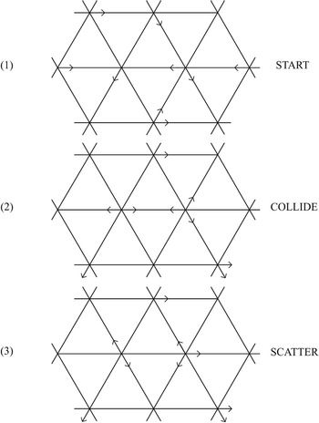
Consider a set of point particles confined to move on a hexagonal lattice. Each particle can move in one of six directions, so we attach a vector to each particle (see fig. 1). The rules are as follows. Between 1 and 2 the particles move in the direction of their arrow to their nearest neighbor site. Then, if the momentum at that site sums to zero, the particles undergo a collision resulting in a jump of 60°, as shown in 3.

Figure 1. Update algorithm for lattice gas. Source: Goldenfeld and Kadanoff (Reference Goldenfeld and Kadanoff1999).
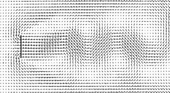
Now take many particles, many iterations of this update algorithm, and perform some coarse-grained averaging to yield macroscopic fields like number and momentum densities. The result will accurately reproduce many of the macroscopic features of fluid flow. In particular, it has been shown that this model reproduces quite accurately the parabolic profile of momentum density that is characteristic of incompressible laminar flow through a pipe (Kadanoff, McNamara, and Zanetti Reference Kadanoff, McNamara and Zanetti1989). Figure 2 gives some idea of how well this model mimics qualitative features of fluid flow past obstacles.

Figure 2. Flow past a flat plate. Source: D’Humières and Lallemand (Reference D’Humières and Lallemand1986).
The LGA is obviously a computational model. Suppose we are interested in studying the behavior of a particular fluid such as water or gasoline as it flows past a plate. We could try to use a computational model that follows the actual trajectories of the molecules that make up the fluid, but it is clear that we would not get very far. Such a model will be woefully inadequate for the purposes of understanding the large-scale structures we are interested in. But we can use the LGA. The question of interest is as follows: Why/how is the minimal model explanatory? What allows us to use it to investigate and to understand the actual behavior of real fluids? It is neither like a continuum model nor like a molecular model. The points in the LGA model are material points representing regions and not molecules. Again, our main question: Why does it work?
Note that the equations of fluid flow (1) and (2) show how the velocity of a fluid at one point in space affects the velocity of the fluid at other points in space. Such an equation results from three fundamental features:
• Locality: A fluid contains many particles in motion, each of which is influenced only by other particles in its immediate neighborhood.
• Conservation: The number of particles and the total momentum of the fluid is conserved over time.
• Symmetry: A fluid is isotropic and rotationally invariant. (Goldenfeld and Kadanoff Reference Goldenfeld and Kadanoff1999, 87)
A common features account would presumably argue that the reason the LGA works is because it shares locality, conservation, and symmetry with the real fluid we are targeting. Some philosophers have extolled the virtues of “minimalist” models along these lines.Footnote 10 For Weisberg, a model is minimalist because it “accurately captures the core causal factors” and because it isolates those factors that “make a difference to the occurrence and essential character of the phenomenon in question” (Reference Weisberg2013, 100–102). For Weisberg, in all cases of minimalist modeling, “the key to explanation is a special set of explanatorily privileged causal factors” (103).
We think it stretches the imagination to think of locality, conservation, and symmetry as causal factors that make a difference to the occurrence of certain patterns of fluid flow or of the fact that the momentum density profile in a pipe is parabolic. But, as we have seen with Pincock, common features need not be causal. And there is a sense in which these common features are clearly relevant. We would like to deny, however, that the explanatory work done by the LGA follows, in any important sense, from these common features alone. The features not mentioned in the model (or those that have been idealized away somehow) will be the “features that are irrelevant.” The common features are to be the relevant ones. But in what respect are they relevant?
Our suggestion is that these minimal common features are relevant in the sense that they are necessary for the phenomenon of interest (e.g., the parabolic momentum profile in a real fluid in a pipe) to occur. Furthermore, we hold that this is different from the claim that it is in virtue of including these common features that the model is explanatory. As we see it, we need answers to the following three questions:
Q1. Why are these common features necessary for the phenomenon to occur?
Q2. Why are the remaining heterogeneous details (those left out of or misrepresented by the model) irrelevant for the occurrence of the phenomenon?
Q3. Why do very different fluids have features (such as symmetry) in common?
Common features accounts completely misdiagnose what makes these models explanatory because they merely assert that the common features are “relevant” and that others are not, without answering Q1, Q2, and Q3. Moreover, simply citing the common features does not in the least say why the LGA minimal model—a caricature of any real fluid—works to understand the macroscopic behaviors of those real fluids. Indeed, those features alone are certainly insufficient to explain the behaviors of real fluids. Simply to cite locality, conservation, and symmetry as being explanatorily relevant actually raises the question of why those features are the common features among fluids. And that is just to raise question Q3. In addition, merely citing these common features fails to tell us why the other heterogeneous details of these systems are irrelevant to their overall behavior—that is, we still need an answer to Q2. We believe we will have an account of why the LGA minimal model is explanatory, when we have answers to each of these three questions.
3.2. Universality and Minimal Models
Suppose we could determine or delimit the class of systems exhibiting the continuum behaviors of fluids from other systems that fail to manifest such behaviors. This would be to delimit the universality class that accounts for the safety of using the Navier-Stokes equations in widely varying engineering contexts. This would be to determine, in effect, the stability of these behaviors under changes in the lower-scale makeup of the systems. We would be able to show that one could perturb the very microstructural details of water to those of gasoline, say, without affecting the common behaviors they display at continuum scales.Footnote 11 Suppose further that the LGA minimal model can be determined to be a member of this class. This would mean that its microstructural details (whatever they are) could also be morphed into that of water or gasoline without changing the continuum scale behaviors. Were all this to be demonstrable, we would then have an answer to why the minimal LGA model can be used to model and explain the behavior of real fluids like water and gasoline: it is in the same universality class. It will, therefore, yield the same continuum scale behavior that any other system in that class will realize—including real fluids.
This talk of perturbation and morphing is deeply metaphorical. But it reflects a kind of robustness or stability that one gets upon being able to delimit the universality class. In fact, the delimitation of the universality class can be made quite precise (and nonmetaphorical) using the mathematics of the renormalization group. The mathematical strategy is complicated, but we think the gist can be made clear quite easily (see Goldenfeld Reference Goldenfeld1992; Batterman Reference Batterman2000, Reference Batterman2002b, Reference Batterman2005, Reference Batterman2010; Kadanoff Reference Kadanoff2000 for discussions).
The idea is to construct a space of possible systems. This is an abstract space in which each point might represent a real fluid, a possible fluid, a solid, and so on. Then on this space one induces a transformation that has the effect, essentially, of eliminating certain degrees of freedom by some kind of averaging rule. Many expositions mention a technique called the Kadanoff block spin transformation. The idea, briefly, is that if one has a lattice of spins, one can replace a collection from within the lattice by an average or block spin that captures, in some way, the interaction among spins in the original system. By rescaling, one takes the original system to a new (possibly nonactual) system/model in the space of systems that exhibits continuum scale behavior similar to the system one started with. This provides a (renormalization group) transformation on all systems in the abstract space. By performing this operation repeatedly, one can answer question Q2 because the transformation in effect eliminates details or degrees of freedom that are irrelevant. Next, one examines the topology of the induced transformation on the abstract space and searches for fixed points of the transformation. If ![]() represents the transformation and p* is a fixed point, we will have
represents the transformation and p* is a fixed point, we will have ![]() . Those systems/models (points in the space) that flow to the same fixed point are in the same universality class—the universality class is delimited.Footnote 12 A derivative, or by-product, of this analysis is the identification of the shared features of the class of systems. In this case, the by-product is a realization that all the systems within the universality class share the common features locality, conservation, and symmetry. Thus, we get an explanation of why these are the common features as a by-product of the mathematical delimitation of the universality class. This answers question Q3 and provides, given the answer to Q2, an answer to Q1—why the common features are necessary for the phenomenon to occur.
. Those systems/models (points in the space) that flow to the same fixed point are in the same universality class—the universality class is delimited.Footnote 12 A derivative, or by-product, of this analysis is the identification of the shared features of the class of systems. In this case, the by-product is a realization that all the systems within the universality class share the common features locality, conservation, and symmetry. Thus, we get an explanation of why these are the common features as a by-product of the mathematical delimitation of the universality class. This answers question Q3 and provides, given the answer to Q2, an answer to Q1—why the common features are necessary for the phenomenon to occur.
Let us make the following important comparison: many explanations focus on finding difference-making factors and implicitly assume that factors left out are irrelevant. In minimal model explanations this process is reversed: one proceeds by showing that various factors are irrelevant. The remaining features will then be the relevant ones.Footnote 13
In figure 3, the lower collection represents systems in the universality class delimited by the fact that these systems/models flowed to the same fixed point, p*, under the appropriate (renormalization group) transformation ![]() in the upper abstract space. Note that another system/model, F +, fails to flow to the fixed point p*, and so that system/model is not in the universality class. Note also, and this is crucial, that the LGA model is in the universality class. The point in the abstract space corresponding to the LGA model does flow to the fixed point. This allows us to understand how such a caricature can be used to explain the behavior of real systems—the remaining heterogeneous details are irrelevant.
in the upper abstract space. Note that another system/model, F +, fails to flow to the fixed point p*, and so that system/model is not in the universality class. Note also, and this is crucial, that the LGA model is in the universality class. The point in the abstract space corresponding to the LGA model does flow to the fixed point. This allows us to understand how such a caricature can be used to explain the behavior of real systems—the remaining heterogeneous details are irrelevant.

Figure 3. Fixed point and universality class.
3.3. Summary
This section presented a minimal model (LGA) that can be used to investigate the behaviors of fluids at everyday (continuum) length and timescales. We have argued that what accounts for the explanatory power of this model is not that it correctly mirrors, maps onto, or otherwise accurately represents the real systems of interest. Instead, the model is explanatory and can be employed to understand the behavior of real fluids primarily because of a backstory about why various details that distinguish fluids and fluid models from one another are essentially irrelevant. This delimits the universality class and guarantees a kind of robustness or stability of the continuum behaviors of interest under rather dramatic changes in the lower-scale makeup of the various systems and models. The renormalization group strategy, in delimiting the universality class, provides the relevant modal structure that makes the model explanatory: we can employ complete caricatures—minimal models that look nothing like the actual systems—in explanatory contexts because we have been able to demonstrate that these caricatures are in the relevant universality class. As such, one might as well use those minimal models for computational ease. The backstory guarantees that, with respect to continuum scale behaviors, it will reproduce the behaviors of real systems.
In order (we hope) to avoid confusion, consider the following two questions and answers:
A. Why does a fluid flowing in a pipe exhibit a parabolic momentum profile? Answer: the particular fluid and the LGA model are in the same universality class, and by analyzing the LGA we can see that all fluids within this universality class will exhibit this profile.
B. Why do the members of the universality class have locality, conservation, and symmetry in common? Answer: the delimitation of the universality class by the renormalization group story (finding the fixed point of the relevant transformation) accounts for this commonality.
Notice that despite the fact these two questions appear different, they are answered in exactly the same way. Thus, to explain why fluids display the continuum behaviors they do, we employ the very same (fixed-point) explanation required for answering the other question; namely, why do the fluids have the common features of locality, conservation, and symmetry? Citing the common features (as relevant difference makers) is in effect just to pose the question one is interested in answering. The real explanatory work is done by showing why the various heterogeneous details of these systems are irrelevant and, along the way, by demonstrating the relevance of the common features. So, we feel that for the kind of ubiquitous explanatory tasks involving understanding how universal behavior is possible, the common features account completely misses what is explanatory. It allows (a version of) the explanandum to masquerade as the explanans.
4. Modeling Biological Populations
Parallel examples of using minimal models to explain various phenomena can be found in biology. In a diverse array of applications, models that are only caricatures of real populations are employed to explain actual biological patterns that range over extremely heterogeneous populations. In such cases, the systems whose behavior we would like to explain typically have very few features in common. However, despite the extreme complexity and heterogeneity of biological systems, biological modelers have been extraordinarily successful at building relatively simple mathematical models to explain the patterns we observe in nature. Such biological models typically make no reference to the details of particular populations whose behavior they purport to explain. Yet, despite their lack of attention to such details, these models can be used to explain many of the patterns we observe across a diverse range of populations (i.e., these models are extremely safe). This is another instance of “universality,” and it can be exploited to find minimal models that can be used to investigate, explain, and understand real biological systems. Indeed, many biological modelers emphasize this kind of universality as a main reason for using their mathematical modeling techniques. For example, Stephens and Krebs note that “foraging theorists have tried to find general design principles that apply regardless of the mechanisms used to implement them. For example, the elementary principles of a device for getting across a river—that is, a bridge—apply regardless of whether the bridge in question is built of rope, wood, concrete, or steel” (Reference Stephens and Krebs1986, 10). In short, there are some large-scale patterns (or macroscale behaviors) that reoccur regardless of the particular physical or mechanistic details of the biological system. In fact, in many cases, a few key parameters within a highly idealized mathematical model will encode all the relevant features of the population. As an example, below we present R. A. Fisher’s model of the sex ratio in which all the relevant dynamics are encoded in the substitution cost for producing male and female offspring. The various details that distinguish the biological populations whose behavior Fisher wanted to explain (e.g., differences in the mechanisms underlying these costs) are irrelevant. Such universal behavior across extremely heterogeneous systems is a primary target for biological theorizing. Fortunately, in many cases this universality means that we can use minimal models to investigate, explain, and understand the behavior of real populations.
4.1. Fisher’s Sex Ratio Model
As we have seen, the aim of a minimal model is to understand the large-scale patterns we observe across systems that are extremely diverse with respect to their smaller-scale details. One such pattern is the widely observed 1:1 sex ratio in natural populations. Fisher (Reference Fisher1930) provided a simple equilibrium model in order to explain this biological pattern (see Hamilton Reference Hamilton1967; Maynard Smith Reference Maynard Smith1979; Charnov Reference Charnov1982; Sober Reference Sober1983, Reference Sober2000, for elaboration and discussion). Although this example has been widely discussed before, we think some of its important features have been either ignored or misunderstood.
Fisher’s original argument is presented in the following passage:
In organisms of all kinds the young are launched upon their careers endowed with a certain amount of biological capital derived from their parents. … Let us consider the reproductive value of these offspring at the moment when this parental expenditure on their behalf has just ceased. If we consider the aggregate of an entire generation of such offspring it is clear that the total reproductive value of the males in this group is exactly equal to the total value of all the females, because each sex must supply half the ancestry of all future generations of the species. From this it follows that the sex ratio will so adjust itself, under the influence of Natural Selection, that the total parental expenditure incurred in respect of children of each sex, shall be equal; for if this were not so and the total expenditure incurred in producing males, for instance, were less than the total expenditure incurred in producing females, then since the total reproductive value of the males is equal to that of the females, it would follow that those parents, the innate tendencies of which caused them to produce males in excess, would, for the same expenditure, produce a greater amount of reproductive value; and in consequence would be the progenitors of a larger fraction of future generations than would parents having a congenital bias towards the production of females. Selection would thus raise the sex ratio until the expenditure upon males became equal to that upon females. (Fisher Reference Fisher1930, 142–43)
In Fisher’s model, the set of available strategies includes all the possible points on a continuum from producing only male offspring to producing only female offspring. In a later paper investigating the key assumptions underlying Fisher’s argument, Hamilton (Reference Hamilton1967) argues that the main idea behind Fisher’s model is that if the population moves away from a 1:1 sex ratio then there will be a fitness advantage favoring parents who overproduce the minority. To see this, suppose that females are more numerous in the population than males. Consequently, parents who overproduce males will, on average, have more offspring contributing to future generations than those who overproduce females. Therefore, parents who overinvest in the production of males tend to receive greater reproductive value for their investment, and male births will become more common in the population. However, as the population approaches a 1:1 ratio, this fitness advantage fades away. The exact same reasoning applies if we assume that female births are less common. Therefore, a 1:1 sex ratio—or, more precisely, equal investment of resources in male and female offspring—is the stable equilibrium state of the evolving population.
Fisher’s model relies on a key trade-off between the ability to produce sons and daughters. This trade-off—which economists refer to as the substitution cost—tells us how many sons can be produced if one less daughter is produced. In Fisher’s explanation of the 1:1 sex ratio, this substitution cost is perfectly linear—males and females cost the same amount of resources to produce, and so one fewer son means one more daughter and vice versa. This is why his model predicts a 1:1 sex ratio. Indeed, the key to deriving the 1:1 sex ratio is that natural selection will lead to equal investment in males and females, and males and females cost the same amount of resources to rear to reproductive age (Sober Reference Sober1983). However, equal investment of resources in male and female offspring will result in other sex ratios if males and females cost different amounts of resources to produce. Indeed, in a later investigation of Fisher’s argument, Charnov (Reference Charnov1982, 28–29) shows that generalizing Fisher’s model leads to the conclusion that the equilibrium sex ratio of a population, r, can be calculated using the following formula:

where CM is the average resource cost of one male offspring and CF is the average resource cost of one female offspring. In other words, this substitution cost is the dominant feature that is the key to understanding the phenomenon Fisher wanted to explain. In fact, Fisher himself recognized that differences in the comparative costs of rearing male and female offspring to reproductive age would result in different sex ratios. As a result, he tried to explain why the human sex ratio is skewed toward males at birth yet also why males are less numerous by the end of the period of parental investment (Fisher Reference Fisher1930, 143). Fisher explained these facts by noting that males cost less to birth but have a higher mortality rate, and so they cost more on average to raise to reproductive maturity. So identifying the commonality of the linear substitution cost allows us (i) to explain the 1:1 ratio across many natural populations, but (ii) by finding this fixed point we can also explain the behavior of other systems near that fixed point—populations that deviate slightly from the 1:1 sex ratio. Moreover, we see that Fisher understood the need to illustrate the relevance of the substitution cost to determining the sex ratio in order to show why his argument could explain the 1:1 sex ratio.
As was the case in the LGA model, a few key parameters encode all the relevant details of these systems.Footnote 14 Moreover, as in the earlier example, we believe that this common feature—the substitution cost—is necessary for the phenomenon (1:1 ratio) to occur. Of course, this makes the substitution cost relevant for the phenomenon to occur. But, we claim, simply stating that common features are relevant features is not sufficient to explain the phenomenon. Indeed, several additional assumptions are operative. In other words, the explanation provided by Fisher’s model is far more (and far less) than the features it has in common with real populations. Indeed, it is only a caricature of real populations.
While Fisher does not make most of these assumptions explicit, later investigations by other authors (including Hamilton, Charnov, Sober, and Maynard Smith) have clarified some of the idealizing assumptions required for Fisher’s derivation of the 1:1 sex ratio. First, the strategy set of Fisher’s model does not accurately represent the set of strategies actually present within any real system. In addition, Fisher’s optimization assumptions are inaccurate when compared with the selection processes taking place in real populations. While the comparative cost of producing male and female offspring is certainly important, this is only one thing that might influence the survival and reproduction of organisms in a population. In fact, the optimization process described by the model does not accurately represent any actual process operating within the real populations whose behaviors we want to explain. Moreover, as with many biological optimality models, Fisher’s model misrepresents the way in which phenotypic strategies are inherited, by assuming that no recombination occurs and that strategies are inherited perfectly by offspring. These idealizing assumptions are often referred to as “asexual reproduction” or “asexual mating” since they avoid the many well-known complications introduced by sexual mating. In addition, like many biological models, Fisher’s model assumes that the population being modeled is infinite (or effectively infinite) and that organisms within the population mate randomly. These idealizing assumptions play an essential role in the model’s derivation of why the optimal trait according to natural selection is expected to evolve in the population. Therefore, these assumptions, like many of the others, are vital to the explanation provided by Fisher’s model. Indeed, without these additional assumptions, the features represented in Fisher’s model are insufficient for deriving the target explanandum.Footnote 15 However, these additional assumptions entail that Fisher’s model drastically misrepresents the dynamics of any real biological population.Footnote 16 Indeed, Fisher’s model describes a selection process that does not (and could not) occur in any real system. Yet, despite its being only minimally accurate with respect to real biological populations, it seems clear that Fisher’s model is explanatory (Sober Reference Sober1983). The important question is why/how the model is explanatory given that it has so few features in common with the real-world systems whose sex ratios it is intended to explain. As Seger and Stubblefield note, optimality models such as Fisher’s are “intentionally caricatures whose purpose is to gain some insight about how a small number of key variables might interact. To the degree that we persuade ourselves that the model represents reality, and that the modeled interactions are general, we have learned something potentially important about how the world might actually work” (Reference Seger, Stubblefield, Rose and Lauder1996, 108).Footnote 17
Given that these models are only caricatures of real biological populations, why and how can they be used to explain and understand the behavior of real populations? Put differently, how can a model that fails to meet even minimal accuracy requirements nonetheless provide a satisfactory explanation? Citing the features the model has in common with real systems fails to provide a satisfactory answer. Moreover, simply noting that those common features are relevant to the explanandum fails to tell us why those features are common and relevant. The answer to these questions, we contend, is that Fisher’s model is a minimal model within the same universality class as the actual systems whose behavior it purports to explain. The key to understanding the explanatory power of the model is to look to the means by which the universality class is delimited and to the demonstration that Fisher’s model is in that class.
4.2. Fisher’s Model as a Minimal Model
In order to see how such a caricature can be used to explain real systems’ behaviors, we require a process for discovering (or demonstrating) why certain dominant features are relevant and why the various heterogeneous features ignored or misrepresented by the minimal model are irrelevant. Citing the common features in Fisher’s model is insufficient to provide the insight we seek. We still need answers to the following three questions:
Q′1. Why are these common features (the linear substitution cost) necessary for the phenomenon to occur?
Q′2. Why are the remaining heterogeneous details (those left out of or misrepresented by the model) irrelevant for the occurrence of the phenomenon?
Q′3. Why do very different populations have these features in common?
In our view, we can use Fisher’s model to explain the 1:1 sex ratio because it is in the same universality class as populations of real species. A common feature of members of this class is the linear substitution cost. However, simply telling us that Fisher’s model has this feature in common with real systems does not explain why those systems exhibit that behavior. For one thing, we want to understand why such diverse biological systems will all have the same substitution cost—that is, we want to know why this feature is a common feature (Q′3). This requires that we delimit the class of systems that will exhibit a linear substitution cost. In this case, we need a story about why a linear substitution cost will be found in such diverse systems (e.g., a story about how such a feature could be “multiply realizable”). Moreover, given the extreme diversity of the systems within the class, in order to answer this question we need a comprehensive story about why all the various details that distinguish those systems from one another do not matter—that is, we need an answer to Q′2. Finally, by showing that all the other details are irrelevant, we can see why only these common features are necessary for the phenomenon to occur—that is, we can see why those features are the relevant ones.
Suppose we could delimit the class of systems exhibiting a 1:1 sex ratio from other systems that fail to display this macrobehavior. This would be to delimit the universality class that can account for the safety of using minimally accurate models, such as Fisher’s, to explain patterns across extremely heterogeneous biological populations. This process would also demonstrate the stability of the 1:1 sex ratio under various changes in the details of those systems. We could then show that one could perturb the very details (or features) of, for example, a population of sheep into those of a population of mule deer without affecting the stable 1:1 sex ratio they display. Suppose further that Fisher’s minimal model can be determined to be a member of this class—indeed, the model population will evolve a 1:1 sex ratio. This would mean that its details and features (whatever they are) could also be morphed into that of actual populations of sheep or mule deer without changing the 1:1 sex ratio. If we could somehow show all this, we would then have an answer to why Fisher’s minimal model can be used to explain and understand the behavior of real biological populations. The minimal model can be used to explain real systems because it is in the same universality class. Moreover, delimiting this universality class is what will provide the modal force to explain why such diverse populations will all exhibit the same macroscale behavior.
In fact, the importance of the robustness or invariance involved in delimiting the universality class can be seen in various attempts by biological modelers to show that, across a wide range of possible systems, the same equilibrium behavior will result. There have been several attempts to demonstrate the robustness of equilibrium behavior with respect to various genetic assumptions. For example, Eshel and Feldman mathematically demonstrate that “phenotypic changes, when determined by long-term genetic dynamics, even with a multilocus genetic structure including recombination, tend to converge in the long term and, with probability 1, to local optima” (Reference Eshel, Feldman, Orzack and Sober2001, 183). In other words, over the long term, the results of evolution by natural selection tend to converge to the predictions made by optimality models regardless of the kind of genetic system involved. These attempts to show that equilibrium behavior will occur even when the genetic assumptions are changed in various ways do important work within the explanatory context of caricature models like Fisher’s. The key part of the explanation of this pattern is in demonstrating that the 1:1 ratio is stable across changes in these genetic assumptions. This information is key to explaining why we see the phenomenon across such heterogeneous systems. Moreover, this robustness allows us to see why we can use Fisher’s model to understand real systems, even though the model is only minimally accurate with respect to those systems.
Several of the other assumptions involved in Fisher’s model can be (and have been) given similar analyses. For instance, optimality models, such as Fisher’s, are frequently used to explain why a wide range of heterogeneous systems have evolved the optimal strategy (or evolutionarily stable strategy) regardless of whether their assumptions veridically represent any processes systems (Rice Reference Rice2013). Instead, a key part of the explanation involves showing that such macrobehavior is stable across various changes in the actual processes involved in the population’s evolution of that equilibrium point. In addition, it is essential to the explanation that we can demonstrate mathematically that the actual population size is irrelevant to the overall behavior of the system above a certain threshold.
In short, there are a number of techniques for demonstrating that a large class of details of particular systems is irrelevant to their macroscale behavior. This is an essential part of the process of delimiting the universality class—by demonstrating that various details are irrelevant, we can also see the class of systems that will display the behavior we are interested in explaining. In such a minimal model explanation, we begin with a space of possible systems. As before, each point in this space represents a different system. In this instance, some will represent real populations and some will represent model populations.
These populations are distinguished by the types of organisms involved, the various assumptions made about the evolutionary dynamics of the system, the population size, and so on. For example, some of the populations in this space might look like this (see fig. 4):
P1. Sheep, linear substitution cost, infinite population, sexual reproduction …

Figure 4. Fixed point and universality class for populations.
P2. Sheep, linear substitution cost, finite population, asexual reproduction …Footnote 18
P3. Mule deer, linear substitution cost, finite population, asexual reproduction …
P4. Fisher’s model population (including infinite population, etc.)
P5. ⋮…

In Fisher’s case, those systems whose equilibrium point is a 1:1 sex ratio are in the same universality class. To delimit this class, we need to use various techniques for showing why the heterogeneous details of various models and real systems are irrelevant to their macrobehavior. Demonstrating this stability will ultimately provide an answer to Q′2: why are the heterogeneous details of these systems irrelevant? Indeed, the investigations outlined above contribute to the project of ultimately delimiting this class, by showing that various details of those systems are irrelevant. In particular, we see that various details about inheritance, the optimization process, the population size, and the particular mechanisms underlying the linear substitution cost are all irrelevant to the evolution of a 1:1 sex ratio. In addition, a by-product of this process will be finding a set of features the members of the universality class have in common—namely, the linear substitution cost. As a result, we are able to see why those features are common features despite the various differences among these systems. That is, we will have an answer to Q′3 just when we can show why various heterogeneous systems will all display a linear substitution cost. In addition, by showing that all the systems in this universality class have those features, we can answer Q′1: why are these common features necessary for the phenomenon to occur? Consequently, we can also explain why other systems that fail to have those features (e.g., bees) will fail to display the macroscale behavior. By showing that the other details of the system do not matter, we can see why the linear substitution cost is the key to the ubiquity of the 1:1 sex ratio. As a result, the minimal model explanation answers the three questions that illustrate the shortcomings of the common features approach. By answering Q′2 via the delimitation of the universality class, we in turn get answers for Q′1 and Q′3. Finally, we also see that Fisher’s minimally accurate model is within the universality class containing the real systems whose behavior we want to explain. This allows us to understand how such a minimally accurate model could be used to explain and understand real systems. We not only answer the essential questions for explaining the ubiquity of the 1:1 sex ratio (even in impossible systems), but we now understand why we are able to use Fisher’s model to explain the patterns we observe in real biological populations.
4.3. Summary
This section presented a minimal model for explaining the ubiquity of the 1:1 sex ratio. However, Fisher’s model is just one case among many—indeed, biological modelers frequently use minimally accurate models to explain patterns across extremely heterogeneous systems. We contend that what accounts for the explanatory power of many of these caricature models is not that they accurately mirror, map, track, or otherwise represent real systems. Instead, these minimal models are explanatory because there is a detailed story about why the myriad details that distinguish a class of systems are irrelevant to their large-scale behavior. This story demonstrates, rather than assumes, a kind of stability or robustness of the large-scale behavior we want to explain under drastic changes in the various details of the system.
5. Conclusion
By way of concluding, we would like to stress one important aspect of explanatory minimal models that has been missed in the literature and that, we believe, has led the common features accounts astray. In the LGA model we wanted to explain various continuum behaviors exhibited by different fluids. Common features accounts would likely cite the fact that the different fluids have locality, conservation, and symmetry in common as explanatorily relevant and maybe even as explanatorily sufficient. However, as we emphasized in section 3.3, this is a mistake. The fact that the different fluids all possess these common features is also something that requires explanation. The explanation of this fact is provided by the renormalization group–like story that delimits the universality class by demonstrating that the details that genuinely distinguish the fluids from one another are irrelevant for the explanandum of interest. This shows both why they all exhibit the same behavior and why they have the common features locality, conservation, and symmetry.
In the context of Fisher’s model, the same thing holds true. The explanandum is the common/universal 1:1 sex ratio observed in diverse populations of species. Were we simply to cite the fact that all these populations have the common feature of linear substitution cost, we would fail to explain this universal behavior. The reason for this is that we can equally well ask why the populations of different species distinguished by different mating strategies, and so on, all exhibit a linear substitution cost and why they display the 1:1 sex ratio. The answer to both questions, again, involves the delimitation of the universality class. This involves the demonstration that the details that genuinely distinguish the different populations (sexual vs. asexual reproduction, etc.) are largely irrelevant for their displaying the observed 1:1 sex ratio pattern.Footnote 19
The conception of universality, and its explanation, was largely developed by condensed matter theorists interested in understanding the fact that different fluids all display the same behavior near their so-called critical points. Physicists, however, are not satisfied to explain this behavior by citing the common features of symmetry and spatial dimension. Consider the following passage from Michael Fisher:
The traditional approach of theoreticians, going back to the foundations of quantum mechanics, is to run to Schrödinger’s equation when confronted by a problem in atomic, molecular, or solid state physics! … The modern attitude is, rather, that the task of the theorist is to understand what is going on and to elucidate which are the crucial features of the problem. For instance, if it is asserted that the exponent [![]() ] depends on the dimensionality, d, and on the symmetry number, n, but on no other factors, then the theorist’s job is to explain why this is so and subject to what provisos. If one had a large enough computer to solve Schrödinger’s equation and the answers came out that way, one would still have no understanding of why this was the case! (Reference Fisher and Hahne1983, 46–47)
] depends on the dimensionality, d, and on the symmetry number, n, but on no other factors, then the theorist’s job is to explain why this is so and subject to what provisos. If one had a large enough computer to solve Schrödinger’s equation and the answers came out that way, one would still have no understanding of why this was the case! (Reference Fisher and Hahne1983, 46–47)
Fisher, in this passage, asserts quite explicitly that citing the features the different systems have in common is just to ask the very question we are trying to answer. This is precisely where we need something like the minimal model explanations presented above. They provide the deeper understanding we seek.
We have argued that there is a class of explanatory models that are explanatory for reasons that have largely been ignored in the literature. These reasons involve telling a story that is focused on demonstrating why details do not matter. Unlike mechanist, causal, or difference-making accounts, this story does not require minimally accurate mirroring of model and target system.
We call these explanations minimal model explanations and have given a detailed account of two examples from physics and biology. Indeed, minimal model explanations are likely common in many scientific disciplines, given that we are often interested in explaining macroscale patterns that range over extremely diverse systems. In such instances, a minimal model explanation will often provide the deeper understanding we are after. Furthermore, the account provided here shows us why scientists are able to use models that are only caricatures to explain the behavior of real systems.