


1. Introduction
Biological and biomedical flows are predominantly pulsatile flows. Be it speech and phonation, medical device design or cardiovascular flows, flow pulsatility is commonplace. Cardiovascular flow is the most well-studied pulsatile flow dating back to the work of Poiseuille in the 19th century. Centuries of study has produced an extensive literature on pulsatile flow through straight and curved pipes, the effects vessel geometry, vessel branching and bifurcation, etc. Nearly all fundamental studies of pulsatile flows have been focused on internal flows. External pulsatile flows, in contrast, have not been extensively studied. A well-characterized, three-dimensional, surface-mounted obstacle produces a variety of fluid dynamics phenomena and provides a platform for understanding external pulsatile flows.
In this study we experimentally and numerically investigate the wake of a surface-mounted hemisphere under highly pulsatile flow conditions and vary the frequency of the flow pulsatility. We define highly pulsatile flow as flow in which the velocity fluctuations are cyclic and of the same magnitude as the mean velocity. Highly pulsatile flow spans a wide parameter space in which the amplitude, frequency, mean velocity and inflow profile shape can all be varied. Holding all other parameters constant we vary the frequency of free-stream flow pulsatility ranging from a low-frequency, quasi-steady regime to a high-frequency pulsatility of the order of the natural vortex shedding that occurs in steady flow of the same Reynolds number ( $Re$) (Tamai, Asaeda & Tanaka Reference Tamai, Asaeda and Tanaka1987).
The parameter of interest is the reduced frequency,  $k$, defined as,
 \begin{equation} k = \frac{Rf}{\bar{u}} = \frac{R}{\bar{u}P}, \end{equation}
where  $R$ is the hemisphere radius,
  $f$ is the frequency of the pulsatility in Hz,
  $\bar {u}$ is the average streamwise velocity and
  $P$ is the period. The value of
  $k$ is varied holding all other parameters constant. The parameters of the pulsatile inflow waveforms are presented in table 1, while a plot of the idealized inflow waveforms is shown in figure 1. The inflow velocity,
  $u$, is normalized by the mean velocity of the cycle,
  $\bar {u}$, and time is normalized by the duration of one period. The range of frequencies was chosen to span from near steady free-stream flow to free-stream pulsatility near the frequency of natural vortex shedding in flows of this type. The range of
  $Re$ was chosen to be relevant to physiological and biological applications, i.e. of the order of 1000. Cardiovascular flows, human phonation and voiced speech, along with some scales of biolocomotion all exist in or near this range of
  $Re$ (Pedrizzetti & Perktold Reference Pedrizzetti and Perktold2003; Liu Reference Liu2005; Erath & Plesniak Reference Erath and Plesniak2010).
Table 1. Inflow parameters and range of reduced frequencies studied.

 $^{\textrm {a}}$Sinusoidal in the direct numerical simulations, near sinusoidal in the experiments.

Figure 1. Sinusoidal free-stream inflow profiles from  $k = 0.01$ to
  $k = 0.2$. Note: experimental inflow profiles had minor deviations from the ideal sinusoidal profiles depicted.
Considering the scarcity of studies on external, highly pulsatile flow and variety of new wake physics observed throughout the range of  $k$ studied, we were motivated to investigate all reduced frequencies both experimentally and numerically. Experiments were performed in a low-speed, pulsatile wind tunnel, along with direct numerical simulations (DNS) which supplement and extend the experiments. Time-resolved particle image velocimetry (TR-PIV) was used to interrogate several cycles for several values of
  $k$ investigated. The highest value of
  $k$ was not achievable in our experiment. Consequentially, it was investigated only using DNS. To assure the validity of the simulations, all values of
  $k$ studied experimentally were simulated.
Given the temporal and spatial resolution available in the DNS we extract additional useful information not attainable in our experimental set-up. Along with the extending the high end of the range of  $k$, the DNS enable us to resolve the incoming boundary layer profiles, visualize the wake structure with three-dimensional vortex identification and compute energy spectra from multiple positions. Using this information we propose a framework for understanding the effects of highly pulsatile flow ranging from steady free-stream wakes to impulsive, single vortex structure production akin to vortex rings. In addition, we identify a remarkable similarity between critical, transitional parameters pertaining to bluff body wakes in highly pulsatile flow and conventional (piston-based) vortex ring production.
To summarize, we investigate the wake of a surface-mounted hemisphere exposed to a highly pulsatile free stream. The frequency of the pulsatility is varied, the effects are observed, and a framework for understanding highly pulsatile wakes is proposed. In § 2, we review the literature related to the topic and provide context for this investigation. In § 3, we describe the experimental set-up, measurement techniques and numerical methods. In § 4, we present and describe the results of the experiments. In § 5, we extend the range of  $k$ with DNS, present boundary layer profiles and wake visualization. In § 6, we examine energy spectra, present a parametric similarity to vortex rings and propose a framework for the free-stream
  $k$ effects of highly pulsatile flow on obstacle wakes. In addition, the benchmarking of the simulations against experiments and accompanying rationale is included in appendix A.
2. Background
To the best of the authors’ knowledge the only published studies concerning three-dimensional obstacles in highly pulsatile flow are our previous articles. Apart from those studies, the background necessary to contextualize this investigation is split between the study of obstacles and the study of impulsively started and oscillatory flows. This section will be composed of a brief summary of our prior work on the topic followed by a review of related topics.
2.1. Our previous studies
In Carr & Plesniak (Reference Carr and Plesniak2016), a surface-mounted hemisphere was subjected to a highly pulsatile free-stream flow at a reduced frequency of  $k = 0.02$. Velocity fields were computed from phase-averaged particle image velocimetry (PIV) in two orthogonal planes which bisect the hemisphere's near wake. Swirling strength,
  $\lambda _{ci}$ (Zhou et al. Reference Zhou, Adrian, Balachandar and Kendall1999), contours computed from the phase-averaged realizations revealed an arch-type vortex structure in the near wake which was phase locked with the highly pulsatile inflow. Figure 2 depicts the arch-type structure in both accelerating and decelerating inflow.

Figure 2. A depiction of the vortex structures in the near wake of a surface-mounted hemisphere in highly pulsatile flow. Accelerating inflow: 1. Approximate line of separation. 2. Incoming boundary layer. 3. Horseshoe vortex system. 4. Starting arch-type vortex. 5. Approximate point of reattachment. Decelerating inflow: progression of propagation upstream through inflow deceleration. (Carr & Plesniak Reference Carr and Plesniak2016).
During accelerating inflow an arch-type starting vortex forms, which during deceleration propagates upstream reaching the midpoint of hemisphere before it is advected downstream in the accelerating flow of the next cycle. It is important to note that the free-stream flow never reverses direction throughout the pulsatile inflow cycle. The mechanism proposed to explain the arch-type vortex's upstream propagation was based on self-induced advection similar to the dynamics observed in vortex rings. A theoretical propagation velocity based on the equation for vortex ring propagation in Saffman (Reference Saffman1970) was computed and compared favourably to the experimental measurements.
Our follow-up paper concerned the effects of obstacle geometry (Carr & Plesniak Reference Carr and Plesniak2017). To determine if the arch-type vortex formation and propagation was unique to a surface-mounted hemisphere, a surface-mounted square prism and cylinder, both of unity aspect ratio, were subjected to a highly pulsatile free-stream flow at  $k = 0.02$. The salient edges of the cylinder and square prism produce local separation bubbles in addition to the wake. For the square prism these local separation bubbles appeared on the two lateral faces as well as the top face, i.e. all faces excluding the windward and leeward faces. In the case of the unity aspect ratio cylinder the only local separation bubble was located on its top surface. These local separation bubbles each produced their own arch-type starting vortex through accelerating inflow which, in turn, propagated upstream during the inflow deceleration along with the large-scale arch-type vortex in the wake, i.e. the same phenomenon as reported for the hemisphere. These additional local arch-type vortices interacted with the large scale arch-type vortex in complex ways; additionally, the change in geometry affects the propagation trajectory and strength of the arch-type vortex. With these additional complexities and dependencies accounted for, the arch vortex formation and propagation in highly pulsatile flow was found to not be unique to a single obstacle geometry widening its range of application.
2.2. Steady flow around surface-mounted obstacles
The complexity which arises when a steady flow or a developing boundary layer encounters an obstacle has been the object of study for many decades. Among the most important precursors to the present study is that of Acarlar & Smith (Reference Acarlar and Smith1987). Through hydrogen-bubble–wire, dye-based flow visualization, and hot-film anemometry they describe the ‘extremely’ periodically shed hairpin vortices originating from the curved free shear layer, along with the standing or horseshoe vortex at the windward junction. Figure 3 is a schematic that depicts the process by which the hairpin vortices are formed – the curved shear layer develops a Kelvin–Helmholtz-type instability and hairpin-shaped packets of vorticity are shed downstream. This work established the topology of a surface-mounted hemisphere's wake. In the same year, a study by Tamai et al. (Reference Tamai, Asaeda and Tanaka1987) produced similar results, offered a detailed quantification of the horseshoe vortex through a range of  $Re$, and, perhaps most importantly, characterized the pairing of hairpin vortices into primary–secondary sets which in turn affects the Strouhal number (
 $St$) of the hairpin shedding. Additionally, Savory & Toy (Reference Savory and Toy1986) characterized the effect of three incoming boundary layer types, denoted ‘rough, smooth and thin’, on the averaged wake of a surface-mounted hemisphere. These three works advanced our understanding of surface-mounted obstacle wakes significantly.

Figure 3. A schematic depiction of the formation of the wake structures (hairpins) produced by a surface-mounted hemisphere. From Acarlar & Smith (Reference Acarlar and Smith1987).
Manhart (Reference Manhart1998) employed large eddy simulation to produce a three-dimensional, time-resolved flow field at  $Re\,{=}\,150\,000$. Through proper-orthogonal-decomposition-based analysis he concluded that the small scales in the flow are most important in the separation process, and only the far wake can be characterized by large-scale, energetic structures, i.e. shear layer roll-up, hairpin-type structures. Kawanisi, Maghrebi & Yokosi (Reference Kawanisi, Maghrebi and Yokosi1993) investigated the topology of the hairpins at high
  $Re$ using three planes of instantaneous two-component velocity data and a mass-consistent model to obtain the third component. They found that at high
  $Re$ the legs of hairpins are not observable but the primary–secondary pairing still exists even in a highly turbulent wake. In addition, many other surface-mounted geometries have been studied including, but not limited to, square prisms (Martinuzzi & Tropea Reference Martinuzzi and Tropea1993; Bourgeois, Sattari & Martinuzzi Reference Bourgeois, Sattari and Martinuzzi2011), pyramids (Martinuzzi & AbuOmar Reference Martinuzzi and AbuOmar2003; AbuOmar & Martinuzzi Reference AbuOmar and Martinuzzi2008), cones (Chen & Martinuzzi Reference Chen and Martinuzzi2018), finite circular cylinders (Pattenden, Turnock & Zhang Reference Pattenden, Turnock and Zhang2005; Sumner Reference Sumner2013), hemispheres of non-unity aspect ratio (Hajimirzaie, Wojcik & Buchholz Reference Hajimirzaie, Wojcik and Buchholz2012; Hajimirzaie & Buchholz Reference Hajimirzaie and Buchholz2013) and spheres (Hajimirzaie et al. Reference Hajimirzaie, Tsakiris, Buchholz and Papanicolaou2014).
Through these and other studies, the flow structures around surface-mounted obstacles in a steady free-stream flow have been characterized thoroughly. The study presented herein ranges from a quasi-steady flow, for which the studies cited above are relevant, to a high-frequency pulsatile flow. To understand the high-frequency pulsatile cases, one must turn to the study of oscillatory and impulsively started flows.
2.3. Impulsively started flows and oscillatory external flows
To understand the high-frequency range, it is helpful to think of a pulsatile flow as a cyclically impulsive flow – a series of impulsive accelerations followed by impulsive decelerations. Impulsive flows have long been known to produce structures not present in steady flow, the most well known of which must be Prandtl's starting vortex. While much of the literature on starting vortices is concerned with airfoils (Mehta & Lavan Reference Mehta and Lavan1975), starting vortices originating from other geometries have also been studied. Additionally, the term ‘starting vortex’ is not often used in oscillatory or other impulsive flows despite observation of flow structures exhibiting the features of a starting vortex – a vortical structure that appears when a flow is accelerated quickly which differs meaningfully from the structures observed under the same conditions in steady flow.
A paper by Pullin & Perry (Reference Pullin and Perry1980) provides several flow visualizations which introduce a typical, non-airfoil starting vortex and compare the observations favourably to similarity theory. Among their motivations they note the close ties between starting flows and vortex rings – a theme closely tied to the findings of our investigation. Lian & Huang (Reference Lian and Huang1989) later investigated starting vortices induced by flat plates, circular discs and hollow hemispheres (with their axis of radial symmetry oriented parallel to the free stream). Through hydrogen-bubble visualization over a range of rates of acceleration and  $Re$, they found the starting vortex evolves to form a threefold structure composed of several small vortices at the outermost layer, a turbulent annular layer and a rotating core. A later study by Johari & Stein (Reference Johari and Stein2002) focused on the near wake of an impulsively started disc and found that an axially symmetric vortex ring is produced in near wake for a brief period. Tonui & Sumner (Reference Tonui and Sumner2011) found similar results around a wide array of two-dimensional square prisms documenting a symmetrical wake structure of starting vortices at
  $Re = 200\text {--}1000$.
Oscillatory flows have been studied extensively, with one of the most influential investigations being Keulegan & Carpenter (Reference Keulegan and Carpenter1956) from which the Keulegan–Carpenter number,  $K_C$, originated. Oscillatory flows at a variety of
  $K_C$ numbers are known to produce coherent vortex structures that can have profound effects on the turbulence dynamics and the surrounding environment (Mei & Liu Reference Mei and Liu1993). Canals & Pawlak (Reference Canals and Pawlak2011) experimentally investigated how a coherent structure in a oscillatory flow breaks down. They proposed, and quantitatively supported, that a combination of elliptic and centrifugal instability is responsible for the breakdown of a columnar vortex pair produced by an oscillating, two-dimensional fence. Geophysical flows as a whole are often unsteady or impulsive. While often of a higher
  $Re$, coastal flows and studies of gusts share some physics with this investigations and could be informed by it (Mei & Liu Reference Mei and Liu1993; Lee et al. Reference Lee, Rho, Kim and Lee2011; Hench & Rosman Reference Hench and Rosman2013).
In addition to steady flows around bluff bodies, oscillatory flows and impulsively started flows there are other fluid dynamics phenomena which provide some background to the present study. Vortex lock-on is one such phenomenon. When studying vortex lock-on experimentally, the frequency of vortex shedding is often manipulated using an external frequency source, sometimes referred to as pulsatility. While this is not highly pulsatile flow, it exemplifies that adding external cyclic forcing can affect vortices and be harnessed for engineering applications (Griffin Reference Griffin1991). Another field of study which influences and could be impacted by the present study is swimming and locomotion. The flow produced in swimming of nearly all kinds contains vortices which are locked-in to the forcing of the animal or machine and creates flow fields which can be considered impulsive (Colgate & Lynch Reference Colgate and Lynch2004).
3. Experimental and numerical methods
3.1. Experimental methods
All experiments were performed in a pulsatile wind tunnel designed and constructed to facilitate these experiments. The hemisphere was 3D-printed on a Formlabs Form 2 stereolithography printer with 140  $\mathrm {\mu }$m resolution and has a radius,
  $R$, of 20 mm. Figure 4 depicts the primary elements of the wind tunnel. The flow enters the settling chamber through a duct which is perforated on the upstream side, facing away from the flow conditioning. The flow conditioning is composed of polycarbonate honeycomb
  $l/m = 8$, where
  $l$ is the length of a cell and
  $m$ is the radius of a cell. The flow then passes through a series of four screens of incrementally decreasing mesh size:
  $2\times 42$ mesh, 0.14 mm wire; 36 mesh, 0.17 mm wire; 30 mesh, 0.17 mm wire. Next, the flow passes through a two-dimensional 5:1 contraction designed using 5th-order polynomial (Bell & Mehta Reference Bell and Mehta1988). After passing through the acrylic test section (
 $150\ \textrm {mm}\times 150\ \textrm {mm}\times 500\ \textrm {mm}$) the flow exits through a diffuser before it is redirected to the seeding confinement chamber.

Figure 4. Depiction of the primary components of the low-speed, pulsatile wind tunnel.
Figure 5 depicts the mechanism which produces the flow pulsatility. After the flow passes through the fan it is directed either through a short duct and into the settling chamber or it bypasses the tunnel and flows back into the seeding confinement chamber. The direction the flow travels is dictated by the position of two butterfly valves attached to a T-junction duct, as depicted in figure 5. The motion of the butterfly valves is synchronized with a tensioned, toothed timing belt. The timing belt ensures that the butterfly valves maintain a 90 $^\circ$ offset such that the combined open area of both valves is constant at all rotational positions, e.g. when one valve is fully open the other is fully closed. The timing belt is also attached to a SureStep STP-MTRH-34127D programmable stepper motor and a Serial Command Language-based controller which drives the rotation of the butterfly valves. Repeatable flow pulsatility can be produced in the test section by rotating or oscillating the butterfly valves at the desired frequency. The amplitude of the pulsatile waveform can be set by adjusting the fan speed.

Figure 5. Depiction of the pulsatility generator.
For the experiments reported herein the butterfly valves were rotated at a constant angular velocity to produce the desired reduced frequency,  $k$, (1.1). To determine the necessary fan speed to produce the required velocity per
  $k$ a Dantec Multichannel constant temperature anemometry (CTA) 54N81 system was used. After calibration, a unidirectional 55P11 hot-wire probe was positioned in the centre of the test section (75 mm from the sidewalls, 20 mm downstream of the test section–contraction junction). Along with monitoring the instantaneous velocity, a running 10 cycle average of the velocity was computed in real time. The fan velocity was then adjusted to achieve the desired full-cycle mean velocity and amplitude. The fan and stepper motor parameters determined using the CTA system were used during the subsequent investigations using TR-PIV.
Table 2 outlines the TR-PIV system details. In figure 4 the position of the various elements of the TR-PIV system are depicted. The laser head was mounted to the optical table along side the wind tunnel. The beam was redirected into the test section using a series of mirrors. To achieve the brightness and repetition rate needed without burning elements of the experimental set-up, a Thorlabs 30:70 cube-type beam splitter was used to redirect 70 % of the laser light into a beam trap. After passing through the beam splitter the beam is optically spread into a sheet and redirected into the test section. The sheet-forming optical elements were chosen such that the sheet was sufficiently wide to cover the area of interest and that the beam waist was centred within the area of interest (Weichselbaum et al. Reference Weichselbaum, André, Rahimi-Abkenar, Manzari and Bardet2016). The beam waist in this case was approximately 0.75 mm and located 0.5  $D$ away from the base plane. The high-speed camera was mounted to the side of the test section and a wide (28 mm) lens was used to obtain the desired field of view (FOV).
Table 2. TR-PIV experimental system details.

The PIV images were captured using IDT Motion Studio software and processed with LaVision DaVis 8.4.0 software. To obtain a suitable particle displacement in the free stream a frame rate of 6 kHz was used, which sets the time between images,  $\textrm {d} t = 164$
 $us$. The frame rate was set on the laser which triggered high-speed camera directly, eliminating the need for external synchronization. To obtain multiple cycles for each value of
  $k$, the total number of frames captured varied between 10 000 for the highest
  $k$ and 20 000 for the lowest
  $k$.
$k$.
Highly pulsatile flows inherently have a large dynamic range of velocities. This flow not only has a large dynamic range through its cycle, but additionally, in some phases, the wake and free-stream regions differ in velocity greatly. To obtain data in all locations with optimal sampling rates would require localized sampling both temporally and spatially – a prohibitively lengthy and complex process. This issue is addressed by employing a sliding averaging process termed, in LaVision DaVis software, the sliding sum of correlation. The first step in this process is to correlate the frame of interest to the next several frames, i.e.  $+1\,\textrm {d} t$,
  $+2\,\textrm {d} t,\ldots$ The set of correlation maps is then averaged with a Gaussian bell curve weighting such that the frames nearer the frame of interest contribute most. This process is capable of producing vectors with a high correlation even with highly dynamic flows such as the one studied herein. From these velocity fields, vorticity was calculated.
3.2. Numerical methods
The pulsatile simulations are carried out using an in-house finite difference Navier–Stokes code, wherein the governing equations for a viscous incompressible flow are discretized on a structured grid in Cartesian space. The geometry of the hemisphere, which is not aligned with the grid, is treated using an immersed-boundary formulation. An exact, semi-implicit projection method is used for time advancement. All terms are treated explicitly using a Runge–Kutta third-order scheme with the exception of the viscous and convective terms in the wall-normal direction. Those terms are treated implicitly using a second-order Crank–Nicholson scheme. All spatial derivatives are discretized using a 2nd order, central-difference scheme on a staggered grid. The code is parallelized using a classical domain decomposition approach. The domain is evenly divided in the streamwise direction and communication between the processed is handed with MPI library calls. The inlet boundary condition is a uniform pulsatile velocity matched with the experiments. The simulations were computed on George Washington University's Colonial One Cluster and used 50 CPU cores. More details of the solver can be found in Beratlis, Balaras & Kiger (Reference Beratlis, Balaras and Kiger2007).
The computational domain, shown in figure 6, measures  $31R\times 30R \times 4R$ in the streamwise, wall-normal and spanwise directions, respectively. The hemisphere is centred at the origin. The inlet and the outlet are located
  $11R$ and
  $20R$ upstream and downstream of the hemisphere. The boundary conditions are no-slip wall at the bottom, slip wall at the top, and periodicity in the spanwise direction. At the outlet a convective boundary condition is used while at the inlet a pulsatile uniform velocity profile is prescribed. The grid contains
  $650\times 280\times 200$ points in the
  $x, y$ and
  $z$ directions respectively. Near the surface of the hemisphere the grid resolution is
  $D_x=0.01R$,
  $D_y=0.01R$ and
  $D_z=0.02R$. The grid resolution is sufficient to capture all the important flow structures. The simulations were initialized with uniform flow and time probes were placed in the flow to monitor the evolution of the transient state. It was found that after approximately
  $100R/U$ time units the flow reached a periodic state.

Figure 6. Simulation domain with prescribed boundary conditions. Not to scale.
4. Experimental results
In this section we will present the experimental results represented as velocity fields with contours of spanwise vorticity on a streamwise, wall-normal plane which bisects the hemisphere. We offer a brief description of the wake topology and important features and will guide the reader through the wake's evolution in a single cycle. Certain phases to be presented were selected from the cycle. These phases are set at even intervals and include critical positions in the cycle, such as minimum and maximum velocity. Figure 7 depicts a single, idealized cycle with the phases represented marked by red dots. For clarity, the phases selected will be referred as, for example, ‘25 % accelerating’, this means 25 % of the accelerating portion of inflow, not 25 % of the rate of change of velocity (see figure 7). In figure 7 the ‘accelerating’ portion of the inflow profile is shaded in red, the ‘decelerating’ portion is shaded in blue.

Figure 7. A single idealized cycle depicting the position of the plotted phases. The accelerating portion is shaded in red and the decelerating portion is shaded in blue. Note: this is not a time plot of the velocity field from the TR-PIV results.
All sets of the realizations presented are instantaneous and sequential. For visual clarity, every other vector is plotted in the wall-normal direction and every fourth vector is plotted in the streamwise direction. There is expected variation between cycles, given that this is a turbulent wake, but the overall physics are similar in each cycle and the cycle presented is typical. The results are ordered by  $k$ and start with the lowest, quasi-steady, value,
  $k = 0.01$, and conclude with the highest experimentally achievable value,
  $k = 0.1$. Each set of realizations is accompanied by a depiction of the corresponding inflow profile in the top right of the figure intended to convey profile shape. These are included to provide a sense of the profile shape variations per
  $k$. The highest studied value of
  $k$, 0.2, was not attainable in the experimental set-up due to mechanical limitations. Therefore, only DNS results will be presented for
  $k = 0.2$ in later sections.
Given the temporal nature of highly pulsatile flows, animated representations often offer advantages over still images. To address this, a series of supplementary movies are available at https://doi.org/10.1017/jfm.2020.659. We encourage the reader to view these movies and compare them with the instantaneous snapshots of velocity and vorticity in §§ 4 and 5. Additionally, the DNS results for each case are presented in the appendix A. Where relevant, we encourage the reader to refer to the DNS results.
Given only a single plane of velocity data, interpreting the wake topology and vorticity distribution requires contextualization. Figure 3 is a useful aid, especially for low values of  $k$ – note the planes of TR-PIV data presented bisect the centre hemisphere so that the vorticity vectors in the head of a hairpin are normal to the data plane. From this FOV the hairpins will appear as a packet of similarly signed vorticity which forms at the downstream extent of the shear layer due to a Kelvin–Helmholtz instability. The
  $Re$ investigated herein is well within the range of
  $Re$ for which figure 3 is relevant. It is not possible to determine the overall shape or completeness of the hairpins from a single plane of TR-PIV data, but considering the robust nature of this wake structure demonstrated in the literature and the DNS results presented in the subsequent sections and appendix A, we can confidently claim that these packets of vorticity correspond to hairpins. Due to the size of the FOV a single hairpin at most can be captured before being convected downstream. Not pictured in figure 3 is the recirculation region which exists between the shear layer and base plane. As with most turbulent wakes this region is characterized by turbulent mixing with little instantaneous organization. In the FOV presented, this region will appear as a distribution of positively and negatively signed vorticity capped by the positively signed vorticity in the shear layer. As the reader progresses through the range of
  $k$, and the flow becomes progressively more dominated by free-stream pulsatility, the flow will gradually transition from resembling figure 3 to resembling figure 2.
The lowest value of  $k$, 0.01, represents a set of quasi-steady velocity fields that exhibits features reported in steady flow. At the minimum value of velocity, nearly stationary in the free stream, figure 8(a), there are some concentrations of vorticity lingering from the previous cycle. While only slightly stronger than the background mixing, these remaining vorticity concentrations show that influence of the previous cycle carries into the next even at this very low
  $k$. As the flow progresses through its accelerating phases (figure 8b–d) the shear layer grows and begins shedding packets of vorticity from its downstream extent – the cross section of a hairpin head can be seen forming at
  $x/D = 1.3$,
  $y/D = 0.5$ indicated with an arrow in figure 8(d). If presented without the knowledge that the free stream was accelerating these velocity and vorticity fields would be nearly indistinguishable from those captured in steady free-stream flow of the same velocity. The same can be said for figure 8(e), at maximum velocity. Only during the decelerating phases does the wake begin to exhibit signs of its transient nature. As illustrated in figure 8(f–h) the shear layer begins to rise above the crest of the hemisphere, also pictured in figure 23(d,h). The turbulence in the wake is swept upstream, interacting with the hemisphere, and convected into the free stream. The vorticity field in figure 8(a) is produced through this interaction. It is important to note that throughout this entire process the only structures that could be characterized as coherent are the hairpin vortices shed during accelerating inflow. The decelerating phases consist entirely of turbulence in the wake, without formation of new coherent structures.

Figure 8. Velocity vectors and contours of spanwise vorticity calculated from TR-PIV images for  $k = 0.01$ with an arrow indicating a hairpin vortex head. The plane bisects the hemisphere in the streamwise direction and is normal to the base plane. Flow is from left to right. The shape of the normalized inflow profile is depicted with the figure title. Refer to figure 7 for phase locations. Animation of full cycle can be found in supplementary movie 1.
When the reduced frequency is doubled, the flow physics change (contrast figure 8 to 9). For  $k = 0.025$ at minimum velocity, figure 9(a), the vorticity remaining from the previous cycle now has some distinguishable structure – see figure 24(a,e) and note the negatively signed vorticity extending upstream of the hemisphere's crest. The negative values of vorticity at
  $x/D = 0.0$ to
  $-$0.5 and
  $y/D \approx 0.7$ suggest a shear layer extending upstream. During the accelerating phases, figure 9(b–d), the primary shear layer extending downstream of the hemisphere develops to a considerably lesser degree. When maximum velocity is reached, a shear layer with some evidence of hairpin shedding can be observed. During early decelerating inflow, figure 9(f,g), the shear layer develops a concentration of vorticity at its downstream most extent. This concentration rolls up, forming a turbulent structure at
  $x/D = 1$,
  $y/D = 0.6$ in figure 9(g) and
  $x/D = 0.75$,
  $y/D = 0.7$ in figure 9(h). The structure is observed more readily in the vector fields than in the vorticity contours. Unlike the previous case,
  $k = 0.01$, the wake and shear layer have some organization during decelerating inflow.

Figure 9. Velocity vectors and contours of spanwise vorticity calculated from TR-PIV images for  $k = 0.025$. The plane bisects the hemisphere in the streamwise direction and is normal to the base plane. Flow is from left to right. The shape of the normalized inflow profile is depicted with the figure title. Refer to figure 7 for phase locations. Animation of full cycle can be found in supplementary movie 2.
When the reduced frequency is again doubled,  $k = 0.05$, the wake exhibits a similar evolution as observed in the previous case. At minimum velocity, figure 10(a), a shear layer again extends upstream. Through acceleration and maximum velocity (figure 10b–e) the shear layer develops and extends roughly 1.25
 $D$ downstream. The signs of the arch-type vortex, again more clear in the velocity field than the vorticity field, appears in late deceleration. Comparing figure 9(h) and 10(h), the arch-type structure appears to have gained cohesion – indicated with an arrow in figure 10(h). The concentration of vorticity at arch-type vortex's head no longer has the areas devoid of vorticity mixed in. While a threshold was crossed when increasing
  $k$ from 0.01 to 0.025, it appears that
  $k = 0.025$ and
  $k = 0.05$ are in largely the same regime.

Figure 10. Velocity vectors and contours of spanwise vorticity calculated from TR-PIV images for  $k = 0.05$. The plane bisects the hemisphere in the streamwise direction and is normal to the base plane. Flow is from left to right. The shape of the normalized inflow profile is depicted with the figure title. Refer to figure 7 for phase locations. Animation of full cycle can be found in supplementary movie 3.
The highest value of reduced frequency in the experiments,  $k = 0.1$, shows just how much influence
  $k$ has. None of the flow fields in figure 11 resembles the previous cases. At minimum velocity (figure 11a) the arch vortex is well defined and circular. Through acceleration (figure 11b–d) the arch vortex loses coherence and what remains of it is convected downstream in the accelerating free stream. When maximum velocity is reached (figure 11e) the beginnings of a new shear layer appear in the near wake. During the early decelerating phases (figure 11f,g) the shear layer extends downstream nearly 1
 $D$, but resembles, if interpreted by the vector field, a single elongated structure. Near the end of decelerating inflow (figure 11h) the elongated structure becomes more compact, producing the arch vortex which is then carried into the next cycle.

Figure 11. Velocity vectors and contours of spanwise vorticity calculated from TR-PIV images for  $k = 0.1$. The plane bisects the hemisphere in the streamwise direction and is normal to the base plane. Flow is from left to right. The shape of the normalized inflow profile is depicted with the figure title. Refer to figure 7 for phase locations. Animation of full cycle can be found in supplementary movie 4.
Through the range of  $k$ experimentally investigated the wake transforms from a familiar open wake to a single structure dominated by the free-stream forcing function. To facilitate comparison between three of the cases, figure 12 provides a side-by-side comparison of four phases from figures 8, 10 and 11. In figure 26, the experimental and numerical instantaneous flow fields are not identical, but the transition to a single structure is observed in both.

Figure 12. Velocity and vorticity fields for  $k = 0.01, 0.05$, and 0.1 shown side by side to facilitate comparison. The plane bisects the hemisphere in the streamwise direction and is normal to the base plane. Flow is from left to right. Animation of full cycle can be found in the supplementary movies – (a–d) in movie 1, (e–h) in movie 3, (i–l) in movie 4.
For reduced frequencies higher than  $k=0.1$ the most interesting transformations begin to take place. Unfortunately, these high
  $k$ values are increasingly difficult to achieve experimentally. The primary limitation is retaining the other inflow parameters (amplitude, mean, shape) when operating at high frequency. For this reason, a series of direct numerical simulations was performed to complement the experiments. Among their many advantages is the ability to retain a sinusoidal profile while operating at very high frequency. DNS was employed extend our study into higher frequencies and take advantage of the more advanced analysis and visualization techniques possible with computations.
The simulation benchmarking can be found in appendix A. While the simulations do not provide an exact match to the experiments, all the relevant physics and wake regime changes are captured. The simulations and experiments both capture the physics and both support the overall claims made.
5. Simulation results and discussion
In this section, we extend and expand upon the experimental results using DNS results. First, we extend the range of reduced frequency to  $k = 0.2$. This sets the reduced frequency of the free-stream forcing within the range of natural shedding of hairpin vortices at
  $Re = 1000$ (Tamai et al. Reference Tamai, Asaeda and Tanaka1987). We encourage the reader refer to the supplementary movies provided. Secondly, we use the high near-wall spatial resolution of the simulations to characterize the pulsatile boundary layer upstream of the obstacle.
Finally, we use a combination of spectral analysis and three-dimensional vortex identification to identify and understand the remarkable transition completed at these high reduced frequencies. We find a regime transition with morphological and spectral similarity to Gharib and collaborators’ formation time for vortex rings. This regime change, along with our past findings’ similarity to some laws of vortex rings, leads us to believe that three-dimensional pulsatile wakes share many of the same physics with vortex rings formed by a piston-driven generator (Gharib, Rambod & Shariff Reference Gharib, Rambod and Shariff1998).
5.1. Extending the reduced frequency range with simulations
As mentioned previously, experimental limitations prevented producing a reduced frequency equal to the  $St$ of the natural hairpin shedding at
  $Re = 1000$. The simulations, with their good agreement in the prior cases, were used to extend the experimental results. Holding all other parameters constant, the
  $k = 0.2$ case was computed. Computing the flow field at this high reduced frequency was critical in understanding the changes observed in the lower values of
  $k$. The regime change, completed at this high value of
  $k$, provides a means of understanding not only the extrema of the range of
  $k$, but all values in between.
In figure 13, the wake is composed primarily of a single structure in all phases. At minimum velocity, figure 13(a), the arch-type vortex is positioned at  $x/D = 0.4$,
  $y/D = 0.7$. The core of this structure contains zero vorticity. Boundary layer vorticity, in blue, is entrained between the primary arch vortex and a smaller structure just upstream. Through accelerating inflow (figure 13b–d) the arch vortex loses coherence, appearing to break up due to external shear forcing imposed by the free stream – likely an elliptic instability (Canals & Pawlak Reference Canals and Pawlak2011). The arch vortex is then convected downstream through acceleration once again. A new boundary layer can be observed forming on the obstacle and baseplane. At this high
  $k$ the remnants of the vortex from the previous cycle appears throughout most of the present cycle, even with this relatively small FOV. At maximum velocity (figure 13e) the boundary layer on the obstacle begins to separate, producing a very thin layer of negative vorticity on the obstacle's surface. As the boundary layer separates and starts forming an arch vortex more clearly (figure 13f;
  $x/D = 0.55$,
  $y/D = 0.4$), the negatively signed boundary layer vorticity has itself begun to lift off the surface forming a small, secondary arch-type vortex. Additionally, the horseshoe vortex at the windward junction of the hemisphere and baseplane begins to form at 25 % decelerating inflow – substantially later than in lower
  $k$ cases suggesting some required time to form. The potential core of the arch-type vortex can be observed in figure 13(g). The negatively signed vorticity continues lifting off the surface and is convected around the primary arch vortex. Finally, in figure 13(h) the full complexity of this structure can be observed: the potential core, the negative vorticity convected into the free stream and the separation region near the crest of the hemisphere.

Figure 13. Velocity vectors (not scaled with velocity magnitude) with contours of spanwise vorticity for  $k = 0.2$ computed with DNS. The plane is oriented streamwise and normal to the wall. Flow is from left to right. The shape of the normalized inflow profile is depicted with the figure title. Refer to figure 7 for phase locations. Animation of full cycle can be found in supplementary movie 5.
While there are many details in the wake to note at  $k = 0.2$ overall the wake is considerably more orderly than for lower reduced frequencies. There is relatively little mixing throughout, and while the structure produced is complex, it is confined to a single vortex system per cycle. Best observed in figure 13(f), between arch vortex systems there is no vorticity, i.e. from
  $x/D = 0.6$ to
  $x/D = 1.75$ vorticity is zero. This is the completion of a regime change. Another means to visualize this change is through three-dimensional vortex identification.
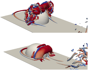
The Q-criterion is a vortex identification technique derived from the velocity gradient tensor,  $\boldsymbol {\nabla } u$, and is defined as a connected region with a positive second invariant (Jeong & Hussain Reference Jeong and Hussain1995). Figure 14 depicts isosurfaces of Q-criterion in the near wake at four phases on inflow for
  $k = 0.2$. The level of the isosurface was chosen to be
  $Q = 15$ to best elucidate the features of the wake. Starting with minimum velocity (figure 14a) the shape and position of the arch vortex is clear even with the turbulent break up process taking place at this phase. The break up process appears to begin at the lateral extremities of the arch vortex and advance inward toward the vortex's midpoint. Moving to 50 % accelerating inflow (figure 14b) the breakup process continues and the small region of coherence at the vortex's midpoint is consumed. At maximum velocity, figure 14(c), two generations of arch vortices can be observed in the same frame. The structure from the previous case, now entirely composed of small-scale structures, is being convected downstream while the next arch vortex forms very near the surface of the hemisphere. Finally, through deceleration the arch vortex, the negatively signed vorticity region, and secondary vortex is formed completing the arch vortex system. The cycle then repeats. To see the temporal evolution of the arch vortex, as viewed through Q, more clearly we suggest the reader view our supplementary movie file.

Figure 14. Q-criterion  $=$ 15 isosurfaces for the
  $k = 0.2$ case. The isosurfaces are coloured by spanwise vorticity. Flow is from left to right. Refer to figure 7 for phase locations. An animation of the figure above can be found in supplementary movie 6.
Additionally, in figure 14(a,c,d), the system of horseshoe vortices is clearly visible. Unlike the regime changes observed in the near wake, the horseshoe vortices undergo only slight morphological changes with increasing  $k$. As with the hairpin vortices in the wake, time is required to develop the complex system of horseshoe vortices. At higher
  $k$, the development of the horseshoe vortex system is limited by the length of a single pulse. The horseshoe vortex system at high
  $k$ retains the horseshoe-like morphology, but does not develop into the full system of multiple vortices (often three or more) which is typically observed in steady flow at the same
  $Re$. The degree and character of the limitation is not discernible from the data presented herein. The localized boundary layer reversal, detailed in the next section, dominates the dynamics of the horseshoe vortices convecting them upstream during decelerating inflow. Fully characterizing the dynamics of the horseshoe vortex system in highly pulsatile flow would require its own investigation.
5.2. Pulsatile incoming boundary layer profiles
In this section we extract boundary layer profiles from the DNS and examine the general trends throughout a single period of each of the reduced frequencies examined. The boundary layer profiles in figure 15 were acquired 3 $D$ upstream of the centre of the hemisphere. The profiles represent
  $u$ velocity and are normalized by the full-cycle mean,
  $\bar {u}$. The dashed line represents the height of the crest of the hemisphere.

Figure 15. Boundary layer profiles for all values of  $k$ from DNS. The phases are those plotted in figure 7. The
  $u$-velocity is normalized by the full-cycle mean,
  $\bar {u}$, and the distance from the wall,
  $y$, is normalized by
  $R$. The dashed line indicates the height of the crest of the hemisphere.
Near-wall reversal in a pulsatile boundary layer is well known, but not well documented. To the best of the authors’ knowledge this is the first high resolution documentation of a flat-plate boundary layer through a sinusoidal, zero-touching, highly pulsatile free-stream velocity profile. Figure 15 is composed of the same phases shown in the previous velocity and vorticity figures, i.e. those marked in figure 7. Starting with perhaps the most interesting phase of the entire cycle minimum velocity, figure 15(a) shows a monotonic increase in the near-wall reversal with increasing  $k$. The quasi-steady case,
  $k = 0.01$, has some minor reversal near the wall but is very near zero velocity throughout. Contrast that with
  $k = 0.2$, where the near-wall reversal is of greater magnitude than the full-cycle mean
  $u$-velocity. For all
  $k$ values between the maximum and minimum, near-wall reversal scales monotonically.
Through accelerating inflow (figure 15b–d) the effects of near-wall reversal diffuse into the free stream at different rates for different  $k$, with no clear trends. Some zones of inflection, e.g.
  $k = 0.025$figure 15(d) at
  $y/R = 0.5$, are due to the presence of the hemisphere. After near-wall vorticity is convected upstream and away from the wall during deceleration it is convected downstream through acceleration leaving imprints on the boundary layer profiles.
The monotonic scaling that occurs at minimum velocity (figure 15a) can be contrasted with the similarity of the boundary layer profiles at maximum velocity (figure 15e). Regardless of reduced frequency, the boundary layer profile when maximum velocity occurs resembles a Blasius profile with some, relatively small discrepancies. The region of near-wall reversal then grows through deceleration for all  $k$, though not monotonically. Some values of
  $k$ outpace others with no apparent trend. Only from 75 % decelerating inflow to minimum velocity does the maximum
  $k$ has the maximum magnitude of near-wall flow reversal.
Of all characteristics of these boundary layer profiles, the dependence on  $k$ at minimum velocity compared with the apparent lack of dependence at maximum velocity must be the most consequential. While not within the scope of this paper, the mechanisms responsible for this difference merit their own investigation.
6. Further analysis and discussion
In this section we plot energy spectral density of pressure fluctuations (ESD $_P$) in the near wake and free stream to observe the changing frequency content, propose a time-dependency explanation and regime map and introduce a non-dimensional parameter for pulsatile flows. We then explore the similarity of this non-dimensional parameter and those used in the study of vortex rings.
6.1. Energy spectral analysis
To observe and quantify the various frequencies present in the flow field ESD $_P$ were computed from the DNS. Two time probes placed in the flow field recorded instantaneous pressure through approximately 20 cycles for each value of
  $k$. One of the probes was placed in the free stream, upstream of the hemisphere (
 $x/D = -3$,
  $y/D = 4$) and the other was placed in the near wake (
 $x/D = 1.0$,
  $y/D = 0.5$). The spectra were computed using the Welch method with 50 % overlap and a Hamming window. The probe in the free stream detects the cyclic changes in pressure due to the free-stream forcing, the pulsatility. The probe in the near wake not only detects the forcing function's pressure fluctuations, but also the pressure fluctuations in the wake due to the presence of the obstacle. Pressure, as opposed to velocity, was chosen because of its greater sensitivity to passing vortex structures. At low
  $k$ we expect the dominant frequencies in the wake to be the pressure signatures of passing hairpins, i.e. the natural shedding observed in steady free-stream flow (see figure 3). Due to the nature of highly pulsatile flow the value of
  $k$ will appear as a peak. Note: the horizontal axis of the spectra in figure 16 is Strouhal number.

Figure 16. Energy spectral density of pressure at two locations. Red: near wake ( $x/r = 2$,
  $y/r = 1$). Blue: in the free stream, upstream of the obstacle. Note: all plots are on the same scale. (a)
  $k = 0.01$, (b)
  $k = 0.025$, (c)
  $k = 0.05$, (d)
  $k = 0.1$ and (e)
  $k = 0.2$.
The energy spectral density calculated from the pressure signals from the two probes is shown in figure 16. For each reduced frequency the ESD $_P$ from the free-stream probe is shown in blue and that from the near wake probe is in red. The spectra for values of
  $k$ were plotted on the same scale to facilitate comparison. In all cases, reduced frequency and probe position, the largest peak is located at the value of St equivalent to
  $k$ for that case, as expected. In all but the
  $k = 0.2$ case that peak is followed closely by harmonics of the primary forcing frequency. Frequencies greater than the forcing function peak and its harmonics reflect the effects of inflow frequency on the wake dynamics.
For the lowest value of reduced frequency,  $k = 0.01$figure 16(a), there is a shallow, broad peak around
  $St = 1$. This peak corresponds to natural shedding frequency in the wake. It is spread over a broad range with no distinct centre because the shedding frequency of the hairpins depends on (varying) free-stream velocity. As this free-stream velocity cycles through accelerating and decelerating inflow the frequency of the natural shedding varies correspondingly over a range. Hence the peak is spread over a range of shedding frequencies. At frequencies higher than this peak,
  $St >1.1$, a cascade of scales is observed.
When  $k$ is increased to 0.025 the peak corresponding to natural shedding becomes less prominent. In figure 16(b) after the primary frequency and harmonics there is a small range, approximately
  $St = 0.2$ to 1.1, where the value of ESD
 $_P$ remains roughly constant. This is followed by a cascade of scales.
Moving to  $k = 0.05$ (figure 16c) no signature of natural shedding can be observed. The primary forced frequency and its harmonics are immediately followed by a cascade of scales. The lack of an additional peak indicates that natural shedding is not present, yet there is clearly wake turbulence in figure 10. For a range of values between
  $k = 0.025$ and 0.05 the free-stream inflow suppresses the natural shedding.
For  $k = 0.1$ the typical profile of a cascade of scales is replaced with a linear region similar to the
  $ESD_P$ in the free stream. This indicates, if interpreted with figures 11 and 26, that the primary vortex structures, although chaotic, are in phase with the forcing function. Finally, in the
  $k = 0.2$ case, the
  $ESD_P$ in the wake and free stream are nearly identical. The arch vortex produced at
  $k = 0.2$ is in phase, organized and compact relative to those produced at lower
  $k$. Due to its compact nature, the arch vortex (or remnants of) narrowly misses the probe position at
  $k=0.2$. With little other turbulent content surrounding the arch vortex, the resulting spectra in the wake and free stream are similar. We refer the reader to supplementary movie 5.
From figure 16 it is clear that varying  $k$ not only affects the dominant forcing frequency, but also impacts the wake physics. The character of the near wake undergoes transformations which can be categorized into several regimes. In the following sections we will propose an explanation of those wake regimes and discuss an important transitional value.
6.2. Wake regimes and time development
One means of interpreting the regimes of the wake is based on the time required for separation to occur,  $T_{sp}$, and the time required to form a shear layer with a Kelvin–Helmholtz instability,
  $T_{kh}$. The length of the period of a pulse decreases with increasing reduced frequency. Within one period there is a subrange in which the
  $Re$ is high enough for separation to occur, i.e.
  $Re > 30$ (Acarlar & Smith Reference Acarlar and Smith1987). In this case, holding fluid properties and obstacle dimensions constant, this
  $Re$ range manifests as a threshold of velocity, denoted
  $U_s$ in figure 17. We will designate this subrange of a period where this dynamics can occur as the functional period,
  $P_f$. For example, the bounds of
  $P_f$ for
  $k = 0.025$ are marked with green circles in figure 17. The temporal duration of this subrange,
  $P_f$, relative to
  $T_{sp}$ and
  $T_{kh}$ is what determines which wake dynamics occurs. In figure 17,
  $P_f$ is the portion of any given period in which the velocity exceeds
  $U_s$, i.e. when
  $Re$ is high enough for separation to occur.

Figure 17. Inflow waveforms with boundaries indicating the time required for the development of boundary layer separation,  $T_{sp}$, the time required for the development of a Kelvin–Helmholtz instability,
  $T_{kh}$, and the
  $Re$ threshold above which separation can occur. These boundaries are placed in their approximate location based on the data in table 3. The functional period,
  $P_f$, is the portion of the period which exceeds the velocity required for separation, denoted
  $U_s$. For clarity, the bounds of the function period for the
  $k = 0.025$ case are marked with green circles. Note: the shaded regions past the lowest and highest values of
  $k$ bounded by dotted lines are artificially extended.
Table 3. Phases of  $T_{sp}$ and
  $T_{kh}$ based on the flow fields presented. The locations of both parameters should be considered approximate, existing within temporal bounds rather than a single value. The positions presented herein are represented graphically in figure 17.

If the times  $T_{sp}$ and
  $T_{kh}$ are short relative to
  $P_f$, the typical wake dynamics present in steady free-stream flow will occur. As
  $P_f$ decreases (with increasing
  $k$),
$k$),  $T_{kh}$ and
  $T_{sp}$ do not decrease proportionally. Instead, with higher
  $k$,
$k$,  $T_{sp}$ and
  $T_{kh}$ take up an increasingly larger portion of
  $P_f$. As the periodic inflow waveform compresses with increasing
  $k$, there is increasingly less time for a typical, steady free-stream wake to develop. In the case of a wall-mounted hemisphere, the emergence of a new structure, the arch vortex, begins where the typical wake structures end.
Figure 17 was developed using the velocity field data shown in figures 8, 9, 10, 11 and 13. Determining an exact time of separation in this turbulent, separated flow is not possible. Instead, the values of  $T_{sp}$ and
  $T_{kh}$ are given within temporal bounds, i.e. between 50 % and 75 % accelerating inflow. This allows direct comparison with the flow fields presented and does not imply a deceivingly precise measurement. The phases in which
  $T_{sp}$ and
  $T_{kh}$ occur are presented in table 3 and are graphically represented in figure 17.
The shaded regions of figure 17 represent the portions of each waveform in which separation occurs (red), and the portion in which the separated shear layer exhibits Kelvin–Helmholtz-type vortex shedding (blue). For lower values of  $k$, i.e. 0.01, 0.025, there is sufficient time during accelerating inflow for both flow phenomena to develop, allowing the wake to take on its typical, steady flow topology. Around
  $k = 0.05$, the separated shear layer begins to develop Kelvin–Helmholtz (K-H) vortices near maximum inflow velocity with inflow deceleration suppressing their development. For
  $k$ higher than 0.05, separation is quickly followed by inflow deceleration without sufficient time for K-H shedding to occur. At high
  $k$ values of 0.1 and 0.2, the arch vortex is the dominant flow feature. Note that the regions in figure 17 below the lowest and above the highest value of
  $k$ bounded by dotted lines are artificially extended.
Figure 18 shows schematic representations of the wake topologies observed at each value of  $k$. Specifically, these represent the final stage of wake development for each value of
  $k$ studied, typically attained near maximum velocity, before inflow deceleration. These representations, along with the flow field data presented in figures 8, 9, 10, 11 and 13, provide a conceptual representation of the changes in the wake as a function of pulsatile frequency.

Figure 18. A map of wake regimes and associated coherent structures in the wake.
As represented in figure 17, the phase in which these flow phenomena occur depends on both time and free-stream velocity. In the case of pulsatile flow, time and velocity are coupled. Consequentially, it is not possible to separate the contributions of time and velocity with the present data. The other important component which dictates the character of the near wake is the degree of impulsivity, or the magnitude of free-stream acceleration. Separating these two parameters, the acceleration and time dependence of the wake, would require its own study.
6.3. Pulsatile convective length scale
Along with a non-dimensionalized frequency (reduced frequency) which serves as a time scale for pulsatile flows, there is similarly a dimensionless length scale associated with all pulsatile flows. During a single period, a fluid packet in the free stream travels a certain distance, ( $\bar {u}*P$). Comparing this convective length to a characteristic length scale gives rise to the pulsatile convective length scale,
  $\ell _p$, defined as,
 \begin{equation} \ell_p = \frac{\bar{u}P}{R}. \end{equation}
 Table 4 contains the values of reduced frequency studied and the corresponding values of  $\ell _p$. As is clear from table 4, the pulsatile convective length scale is simply the inverse of the reduced frequency. Parameters very similar to this can be found in literature on oscillatory flows and vortex rings. Comparison with these other parameters and the dynamics associated with them offers insight into the wakes studied herein.
Table 4. Pulsatile convective length scale values for each reduced frequency.

One of the dimensionless parameters composed of very similar terms is Gharib and collaborators’ formation time,  $T^*$ (Gharib et al. Reference Gharib, Rambod and Shariff1998). Well known in the study of vortex rings, formation time is defined as
 \begin{equation} T^* =\frac{ \bar{U}_p t}{D}, \end{equation}
where  $\bar {U}_p$ is the average piston velocity,
  $t$ is the discharge time and
  $D$ is the orifice diameter. Both
  $T^*$ and
  $\ell _p$ contain an average velocity multiplied by a time over a length.
A typical method employed to form vortex rings experimentally, including that used in Gharib et al. (Reference Gharib, Rambod and Shariff1998), is a sharp edged piston that ejects a plug of fluid. Figure 19 is a schematic comparison of a piston-based vortex ring generator and a hemisphere in pulsatile flow. It is clear that these flow configurations differ in many substantive ways, yet, as we will discuss, similar transitions occur at similar values of key parameters – described by  $T*$ and
  $\ell _p$ for the piston-based vortex ring generator and obstacle in pulsatile flow, respectively.

Figure 19. A schematic comparison of the directionality of primary flow and ring propagation direction. The classic sharp-edged, piston-based vortex ring generator (a), and the surface-mounted hemisphere in pulsatile flow (b).
When  $T^* \approx 4$, as reported in Gharib et al. (Reference Gharib, Rambod and Shariff1998), the total vorticity contained within a single, confined vortex ring reaches its maximum possible (saturated) value without shedding vorticity into its wake. For
  $T^*<4$ the amount of vorticity in the vortex ring decreases linearly. For
  $T^*>4$ the vortex forms a tail containing additional vorticity while the amount of vorticity contained in the ring remains constant at the saturated value achieved at
  $T^* \approx 4$.
Thinking of  $\ell _p$ as a similar parameter we approach from values greater than
  $\ell _p \approx 4$ in which an open wake exists with vorticity distributed over a large area accompanied by the arch vortex. When
  $\ell _p = 5$ (where
  $k = 0.2$, see table 4), the arch vortex produced is a single coherent structure without significant additional, proximal vorticity, as was the vortex ring when
  $T^* \approx 4$. This suggests the arch vortex in the wake of an obstacle in highly pulsatile flow is subject to a similar transition as a vortex ring ejected from a piston. Furthermore,
  $\ell _p$ and
  $T^*$ describe the same set of dynamics despite arising from such disparate geometries and flow conditions. This leads us to predict that if
  $\ell _p$ were decreased further, less than a value of 5, the amount of vorticity contained in the arch vortex would monotonically decrease, i.e. the same relationship between the amount of vorticity contained in a vortex ring and
  $T^* < 4$. While the ‘time required to produce’ framework partially explains the wake dynamics observed, the degree of impulsivity, i.e. the rate of acceleration during accelerating inflow, is certainly another aspect of the explanation. In the present study, the reduced frequency and the rate of accelerating inflow are coupled. Separating these two parameters would require its own investigation – likely one involving varying accelerating inflow rates which are not followed by a deceleration.
Beyond the empirical evidence of a wake regime change near  $\ell _p = 5$, there is intuitive understanding to be gained by considering the critical value of
  $\ell _p$. As with many dimensionless parameters,
  $\ell _p$ is a measure of the relationship of two quantities – in this case a comparison of the distance a fluid packet in the free stream travels in one pulse to a geometric characteristic length. When these two values are very similar, i.e. a pulse moves the fluid only a few obstacle radii, one would expect the resulting fluid structures to be altered. Specifically, one might expect them to resemble the fluid structures observed in impulsively started flows, i.e. to resemble a starting vortex. Furthermore, if these short, rapid accelerations of the fluid or the solid object are cyclic and closely spaced in time (high values of
  $k$ with correspondingly low values of
  $\ell _p$), one could expect several of these starting vortices (or their remnants) to remain in the near wake because they are not convected far downstream.
The numerical transitional value of  $\ell _p$ depends on its definition. In this case, the typical definitions of the length scale, i.e. radius or diameter, can change the value of
  $\ell _p$ by a factor of two. We chose the radius of the hemisphere as it this is the customary characteristic length used in the study of surface-mounted hemispheres. If instead the length scale chosen were diameter, resulting in a transitional value of
  $\ell _p = 2.5$, the resultant claims would still remain valid. The flow phenomena observed both herein and in the study of vortex rings centres around the relationship between the vortex-producing geometry and distance travelled by the impulsive flow.
While transitional values of  $\ell _p$ and
  $T^*$ are very similar, there are some interesting differences between the two flows. One significant difference is the cyclic pulsatility in the presently studied case and the impulsive flow produced by the piston-based vortex ring generator. From the dynamics observed herein, cyclic pulsatility can be treated as a series of discrete impulses. Due to the relative scale and dominance of the free-stream pulsatility over the wake dynamics, effects of temporally adjacent pulses do not appear to have a large effect on the wake dynamics observed within a single pulse, i.e. the vortices produced in a single pulse are convected many hemisphere diameters downstream and do not appear to interact with the vortices produced in the next pulse. Though this may not be true at higher reduced frequencies when the value of
  $\ell _p$ approaches unity and the distance between the structures produced by each pulse lessens.
Another significant difference between the flow configuration is the relative direction of the primary flow and the vortex ring propagation direction. As shown in figure 19, the typical method for producing vortex rings is composed of a piston which ejects a plug of fluid. The vortex ring propagates in the same direction as the fluid ejection. In the present study, the arch vortex (taken with the image of the arch vortex in the ground plane) are produced in such a way that they oppose the primary flow direction. As detailed in Carr & Plesniak (Reference Carr and Plesniak2016), the upstream self-induced propagation direction, along with the near-wall boundary layer reversal, account for the unexpected upstream motion of the wake/arch vortex during decelerating inflow. Assumed in these prior studies, and the present comparison of  $\ell _p$ and
  $T^*$, is validity of the image of the arch vortex. In a separated, turbulent wake the effects of image vorticity may be less clear. Recent works including that of Limacher, Morton & Wood (Reference Limacher, Morton and Wood2018) bolster such a claim.
An additional difference between a traditional vortex ring generator and our set-up is the geometry which produces the initial shear layer. When producing vortex rings a sharp edge to define a separation is often necessary. The lack of any sharp edges on a hemisphere to fix separation further illustrates the robustness of this phenomenon. In addition, there is little documentation of starting vortices produced from smooth bodies, i.e. without a prescribed separation point. Only the waveforms corresponding to higher values of  $k$, 0.1 and 0.2, have the impulsivity required to produce a starting vortex, but in those cases the starting vortex is reliably produced. In past studies we have found that salient edges can have an effect on the trajectory and dynamics of the arch vortex, but they are not required to produce it (Carr & Plesniak Reference Carr and Plesniak2017)
Gharib et al. (Reference Gharib, Rambod and Shariff1998) state that ‘The formation of vortices  $\ldots$ usually involves boundary layer separation and ejection of a column of fluid from a confined volume’. For the surface-mounted hemisphere there is certainly boundary layer separation but not ejection from a confined volume. Thus, the present study expands the applicability of the principles learned from vortex ring generators to highly pulsatile wakes of surface obstacles – a relationship that is unintuitive and not previously reported.
In nature or industrial applications a highly pulsatile flow will fall somewhere on the spectrum of reduced frequency. If it falls near the low end, the wake dynamics will be nearly the same as in steady flow. Near the high end, the wake may consist of only a single vortical structure. Somewhere in between, a separation may occur and, if a little higher, a turbulent wake with some K-H shedding in the shear layer. This regime map, which has not been previously reported, will serve as a useful reference for researchers or engineers studying highly pulsatile flows.
7. Conclusion
The wake of a surface-mounted hemisphere in highly pulsatile flow was investigated experimentally and numerically. The reduced frequency of pulsation was varied from a low-frequency, quasi-steady regime to a high-frequency, impulsive regime. At low  $k$ the wake resembles a steady inflow wake with a free shear layer and hairpin vortex shedding with little organization during decelerating inflow. At moderate
  $k$ hairpin-type shedding was no longer present, leaving only wake turbulence during accelerating inflow. During decelerating inflow, at moderate
  $k$, the wake is more organized into an arch-type structure. At the highest experimentally achievable
  $k$ the wake is nearly entirely replaced by a single arch vortex with some wake turbulence.
We used DNS to extend the range of  $k$, characterize the incoming boundary layer, and visualize the wake structure in three-dimensions. The boundary layer profiles reveal a direct, positive relationship between the magnitude of near-wall flow reversal during decelerating inflow and
  $k$, as well as a lack of interdependence at maximum velocity. At the highest
  $k$ investigated, 0.2, the arch vortex is a single, coherent structure with very little surrounding turbulence. When visualized with Q-criterion, the arch vortex breakdown begins at its lateral extremities and travels inward. Energy spectral density of pressure was computed from probes placed in the near wake and free stream. The energy spectral density profiles reflect the relationship between wake structure and
  $k$ observed in the flow fields – natural shedding and wake turbulence decreasing with increasing
  $k$.
$k$.
We propose that the wake physics are dependent on two development time scales: the time required to develop boundary layer separation and the time required to develop Kelvin–Helmholtz shedding. As  $k$ increases the length of a single period becomes smaller than one or both of these time scales. This splits wake up into a series of regimes, a map of which has been presented. Finally, a length scale which compares the distance travelled by a single fluid packet in the free stream to the characteristic length of the obstacle has been proposed and termed the pulsatile convective length scale,
  $\ell _p$. Remarkably,
  $\ell _p$ appears to describe the same physics and critical value for highly pulsatile wakes as the formation time,
  $T^*$, does for vortex ring generation reported in Gharib et al. (Reference Gharib, Rambod and Shariff1998). The similarity in these relationships expands the knowledge gained in the study of vortex rings to highly pulsatile wakes of surface obstacles.
The phenomena and conceptual framework introduced herein present several opportunities for future studies. Investigating the characteristics of circulation throughout the range of reduced frequency is the clearest opportunity for future work. With a rigorous calculation of circulation of both the hairpins, at low  $k$, and arch, at high
  $k$, direct comparison with the Gharib et al. (Reference Gharib, Rambod and Shariff1998) circulation phenomena, along with calculation of theoretical self-induced propagation velocity, as performed in Carr & Plesniak (Reference Carr and Plesniak2016) would be possible. Additionally, a focused study of the dynamics of the junction vortex system under highly pulsatile conditions would likely produce results of interest. These opportunities, along with several others, could shed light on this relatively unstudied set of flow conditions.
Declaration of interests
The authors report no conflict of interest.
Supplementary movies
Supplementary movies are available at https://doi.org/10.1017/jfm.2020.659.
Appendix A. Benchmarking
In this section we will present the validation of the DNS against experiments. The validation is composed of two parts: (i) a benchmarking case from which boundary layer profiles will be quantitatively compared and, (ii) a series of velocity and vorticity fields from the experiments and simulations presented herein which establish the similarity in the wake features.
A.1. Boundary layer profile validation
To validate the numerical solver, a series of phase-averaged DNS was computed to compare with the phase-averaged PIV at  $k = 0.02$ – within the range discussed in the present study. The phase-averaged PIV data used for validation were originally published and discussed in Carr & Plesniak (Reference Carr and Plesniak2016). With the focus of benchmarking, a series of DNS were computed using inlet conditions that match those measured in the experiments using a Dantec MiniCTA positioned in the free stream. Apart from the CTA-based inlet condition, the domain and boundary conditions match those described in figure 6. To match the parameters of the PIV data, the simulation data were phase averaged over 100 cycles. For more information on the experimental set-up, data processing and physics observed refer to Carr & Plesniak (Reference Carr and Plesniak2016).
From the phase-averaged PIV data and phase-averaged DNS, a series of boundary layer profiles have been measured at three positions all centred on the hemisphere in the spanwise direction,  $x/D = -1, 1, 2.5,\ z/D = 0$. Each position has its own set of physics which need to be captured by the DNS. The upstream position,
  $x/D = -1$, is influenced primarily by the incoming boundary layer and some effects from the horseshoe, or necklace, vortex. The first downstream position,
  $x/D = 1$, is positioned in the near wake, recirculation zone, and the associated mixing and turbulence. The second downstream position,
  $x/D = 2.5$, is slightly downstream of flow reattachment for the majority of the cycle.
For each position four phases from the cycle were extracted. The relative positions of the phases are labelled using the same nomenclature established in figure 7. Due to the choice of phases used in the phase averaging, the exact positions of maximum velocity, minimum velocity, 50 % accelerating and 50 % decelerating, were not captured. The phases nearest to the positions in the inflow waveform were used – one result of which is the difference in free-stream velocity at 50 % accelerating inflow and 50 % decelerating inflow. The experimental boundary layer profiles were composed of a series of discrete positions and interpolated to form a smooth curve. The boundary layer profiles were normalized by the free-stream value at each phase.
In figures 20–22 the boundary layer profiles measured experimentally are represented by the dashed lines and simulation profiles are represented with solid lines. The degree of agreement varies with phase, but in general we expect the boundary layers to be thicker in the experiments than those captured by the simulations. Experimental imperfections such as wall roughness, the boundary layer growth in the contraction, the tape at the seam which joins the contraction and test section are all likely contributors to the generally thicker experimental boundary layers.

Figure 20. Boundary layer profiles 1 $D$ upstream of the obstacle's centre (
 $x/D = -1$). Dashed lines indicate PIV data, solid lines indicate DNS data. The velocity is normalized by the full-cycle mean and the distance from the wall by the hemisphere's diameter. Refer to figure 7 for phase locations.

Figure 21. Boundary layer profiles 1 $D$ downstream of the obstacle's centre (
 $x/D = 1$). Dashed lines indicate PIV data, solid lines indicate DNS data. The velocity is normalized by the full-cycle mean and the distance from the wall by the hemisphere's diameter. Refer to figure 7 for phase locations.

Figure 22. Boundary layer profiles 2.5 $D$ downstream of the obstacle's centre (
 $x/D = 2.5$). Dashed lines indicate PIV data, solid lines indicate DNS data. The velocity is normalized by the full-cycle mean and the distance from the wall by the hemisphere's diameter. Refer to figure 7 for phase locations.
In figure 20, the incoming boundary layer profiles are plotted. The PIV-based profiles are thicker than those from the simulation. Agreement is best at minimum velocity with the inflectional nature of the profiles captured well. The maximum velocity and 50 % decelerating inflow boundary layer profiles both contain a small velocity overshoot at roughly  $y/D = 0.2$ which is not observed in the experimental curves. These discrepancies are within the range expected given the experimental imperfections.
The boundary layer profiles in the near wake, figure 21, agrees reasonably well. The large scale inflections are captured well in each phase. The development of the near wakes region of flow reversal is captured. The increased spatial fidelity of the simulations produces profiles with more small-scale features, especially in the recirculation zone ( $y/D < 1$). As with the other measurement positions, the PIV-based boundary layer profiles are generally thicker than those from DNS.
The velocity profiles in figure 22 are positioned downstream of the point of flow reattachment. The agreement is best at maximum velocity in which the momentum deficit due to the obstacle is clearly defined. The agreement at minimum velocity and 50 % accelerating inflow agree acceptably, but not as well. The phase at which the simulations and experiments disagree most is 50 % deceleration. This is likely due to the extreme sensitivity in capturings the recirculation bubble. As the free-stream velocity varies the streamwise extent and total volume of the recirculation bubble varies. The disagreement in figure 22, 50 % dec. is likely caused by the recirculation bubble in the experiments extending downstream slightly further in this phase. While there is some disagreement, the overall agreement is sufficient to support the claims made herein.
A.2. Velocity field and wake feature comparison
In this section the experimental results and DNS will be shown to have the same essential physics and experience the same changes as we traverse reduced frequency. It is important to keep in mind that the flow fields shown are instantaneous snapshots of a turbulent wake. We do not expect the velocity or vorticity fields to match exactly. What we expect to see is that the same essential physics is captured and the large-scale wake topology is similar. Additionally, the waveform prescribed in the DNS was an ideal sinusoid. The inflow waveform in the experiments, while retaining the amplitude, frequency, and mean, were not perfectly sinusoidal due to mechanical limitations. One manifestation of the discrepancies in inflow profile shape is the appearance of a phase shift between experiments and simulation. While this means the experiments and simulations will have discrepancies, we assert that, for the claims made herein, the simulations and experiments both support the argument.
Both the DNS and TR-PIV results are represented by a velocity field and contours of vorticity on a streamwise, wall-normal plane which bisects the hemisphere. In the DNS representations the arrows indicating velocity are of uniform length and do not represent the magnitude of velocity, only the direction, while the TR-PIV velocity vectors are scaled to represent velocity magnitude. Additionally, the zero value of the colour map is not white in the DNS realizations but a light grey. These differences are due to visualization software limitations and do not represent anything meaningful in terms of flow physics. For each value of  $k$ a single cycle will be represented by four evenly spaced phases which again include maximum and minimum velocity, reference figure 7. We suggest the reader refer to the supplementary movie files for both the TR-PIV data and DNS data for further visualization and comparison.
Starting with  $k = 0.01$, figure 23, at minimum velocity, panels (a,e), the lack of discernible flow features and vorticity is captured well. Moving to 50 % accelerating inflow and maximum velocity, figure 23(b,f) and (c,g) respectively, the shear layer is observed to grow from the crest of the hemisphere and extend downstream, where it shows signs of shear layer roll-up and hairpin shedding. Finally, the shear layer lifts up but contains little in the way of coherent vortex structures.

Figure 23. A comparison of vector fields with spanwise vorticity contours calculated from TR-PIV (a–d) and DNS (e–h) for  $k = 0.01$. The plane is oriented streamwise and normal the base plane. Flow is from (a–h). Refer to figure 7 for phase locations. Animation of full cycle can be found in the supplementary movies – (a–d) in movie 1, (e–h) in movie 7.
In figure 24, a similar progression is observed. Little discernible organization at minimum velocity gives way to a shear layer growing downstream through 50 % acceleration and maximum velocity. The shear layer then rises up during deceleration. The notable difference between  $k = 0.01$ and
  $k = 0.025$ is the shorter downstream extent of the shear layer in figure 24. Again, these are instantaneous snapshots of a turbulent wake so the full extent of the shear layer before it breaks up into hairpin vortices likely varies cycle to cycle. That being said, the shorter duration of a single period is expected to constrain the downstream growth of the shear layer and wake in general.

Figure 24. A comparison of vector fields with spanwise vorticity contours calculated from TR-PIV (a–d) and DNS (e–h) for  $k = 0.025$. The plane is oriented streamwise and normal the base plane. Flow is from (a–h). Refer to figure 7 for phase locations. Animation of full cycle can be found in the supplementary movies – (a–d) in movie 2, (e–h) in movie 8.
As  $k$ increases the discrepancies between the simulations and experiments begin to increase because of the different inflow waveforms. While the large-scale trends agree well, the exact comparison has some discrepancies, but the overall flow physics exhibit acceptable agreement. In figure 25(a,e), the small negatively signed shear layer can be seen extending from the crest of the hemisphere. The shear layer again begins to grow then rise up, capping the region beneath, through maximum velocity and 50 % decelerating inflow, figure 25(c,g) and (d,h) respectively.

Figure 25. A comparison of vector fields with spanwise vorticity contours calculated from TR-PIV (a–d) and DNS (e–h) for  $k = 0.05$. The plane is oriented streamwise and normal the base plane. Flow is from (a–h). Refer to figure 7 for phase locations. Animation of full cycle can be found in the supplementary movies – (a–d) in movie 3, (e–h) in movie 9.
Finally, in figure 26 the consolidation of the wake into a single structure is observed in both the simulations and experiments. The differences in position between the experiments and simulations are again attributable to differences in waveform shape. Additionally, the overall size and shape is captured well by the simulations. Throughout the entire cycle the arch vortex extends less than 1 $D$ downstream. As the structure moves upstream during deceleration the primary arch vortex is accompanied by negatively signed vorticity upstream as well as secondary, positively signed vorticity upstream of that.

Figure 26. A comparison of vector fields with spanwise vorticity contours calculated from TR-PIV (a–d) and DNS (e–h) for  $k = 0.1$. The plane is oriented streamwise and normal the base plane. Flow is from (a–h). Refer to figure 7 for phase locations. Animation of full cycle can be found in the supplementary movies – (a–d) in movie 4, (e–h) in movie 10.


