


I. INTRODUCTION
Airborne passive location of fixed (or slow moving) ground-based emitters has been historically achieved by means of triangulation algorithms. Moving triangulation, or bearing only method [Reference Becker1], is based on several direction of arrival (DOA) measurements achieved by the airborne platform at different times, and therefore from different positions.
Other methods based on frequency measurements as the differential Doppler [Reference Levanon2, Reference Chestnut3] are now becoming interesting, thanks to digital signal processing (DSP) advances that allow very accurate estimation of the received frequency.
In both cases, due to the inaccuracy of the measurements (bearing or frequency), a distance of some tens of kilometers between measuring points could be needed to achieve the wanted location accuracy. Therefore the location is completed only when the aircraft has moved for such a distance, requiring some minutes. When a shorter location time is needed, in the order of a few seconds, combined methods [Reference Becker1, Reference Deng, Liu, Jiang, Zhou and Xu4] have to be considered.
In the framework of a Research and Development (R&D) contract with the Italian Ministry of Defence (MoD), Elettronica SpA (ELT) carried out the theoretical study of a Doppler-based passive location technique and experimented with the selected technique during a field test campaign. The tested location technique is a combined method based on Doppler effect measurements together with DOA measurements. The Doppler effect has been evaluated in terms of frequency difference of arrival (FDOA) of the radio frequency (RF) signal at two receiving antennas positioned at a distance of a few meters on the platform. The DOA has been evaluated through time difference of arrival (TDOA) algorithms to best exploit the two antennas setup needed for FDOA measurements. The concept of the experimented location technique is represented in Fig. 1. The FDOA information defines a curve of compatible emitter positions (iso-FDOA curve). The DOA information defines, at the same time, an axis for compatible emitter positions. The two conditions together allow one to identify the emitter position as the interception of the iso-FDOA curve with the direction of arrival axis.

Fig. 1. Combined location technique based on FDOA and DOA measurements.
II. THEORETICAL STUDY AND SIMULATION
A) Passive location technique
The selected location technique combines two methods, FDOA together with TDOA. Both FDOA and TDOA are differential measures, and they are achieved by positioning two receiving antennas at a distance of a few meters on the aircraft to form a large base interferometer (LBI). Figure 2 shows the geometrical situation.
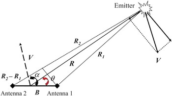
Fig. 2. LBI and emitter reciprocal position for location technique concept description.
The two antennas of the LBI, freely installed on the aircraft, will receive the signal from an emitter at range R with bearing ϑ.
The LBI will then move with a given speed having modulus V and orientation α measured with respect to the LBI. The motion of the LBI will induce a rotation on the line-of-sight of the emitter. The line-of-sight angular velocity will be given by the following expression:
The ![]() depends on the component of V orthogonal to the line-of-sight and on the distance LBI–emitter. The range can then be obtained by inverting (1):
depends on the component of V orthogonal to the line-of-sight and on the distance LBI–emitter. The range can then be obtained by inverting (1):
Therefore when the modulus and the orientation of aircraft speed are known, the estimation of the angle of arrival ϑ together with the estimation of the line-of-sight angular velocity ![]() lead to an estimate of emitter range. The location of the emitter is thus completed.
lead to an estimate of emitter range. The location of the emitter is thus completed.
The angle of arrival ϑ can be obtained by measuring the time difference of arrival of the emitter signal at the two receiving channels associated to the two antennas of the LBI. The geometric situation for TDOA evaluation is illustrated in Fig. 3. In the applications of interest the emitter range compared with the LBI base B is such that the following expression holds:

Fig. 3. DOA evaluation through TDOA measurements.
The line-of-sight angular velocity ![]() can be obtained by measuring the FDOA of the emitter signal at the two receiving channels associated to the two antennas of the LBI. Referring to Fig. 2, the FDOA will be given by
can be obtained by measuring the FDOA of the emitter signal at the two receiving channels associated to the two antennas of the LBI. Referring to Fig. 2, the FDOA will be given by
where f d1 and f d2 are, respectively, the Doppler frequencies at the two antennas and λ is the emitter wavelength. When R ≫ B the following expression holds:
Therefore, inverting (5), we have
The line-of-sight angular velocity can then be estimated through FDOA measurements jointly with emitter frequency information (f) and angle of arrival information.
The emitter range will then result from the combination of (2) and (5):
Equations (7) and (3) allow one to complete the location in two dimensions. The third dimension, given by aircraft height, has not been taken into account for the sake of simplicity, since in nearly all cases it can be neglected.
B) Errors analysis
The sensitivity of the range to the various parameters is obtainable by evaluating the partial derivatives of R(ϑ, FDOA, f, V, α). When the errors on the parameters are uncorrelated and not biased, the variance of the estimated range is a function of the parameters' variance as shown below:
The sensitivity to the different parameters is given in the following expressions:

By means of some algebraic manipulations from (8) and (9), we obtain
The standard deviation σϑ of the measurement of the angle of arrival will be given by
T rise and SNR in (11) are, respectively, the rise time of the pulse video envelope and the signal-to-noise ratio of the received signal as described in [Reference Skolnik5]. N represents the number of pulses on which the measurement is averaged.
The standard deviation σFDOA of the measurement of the FDOA will be given by
The value σFDOA/√2 used for (12) has been derived in [Reference Rife6] for a single frequency estimation over a continuous interval of duration T m in which M samples are collected. However it is possible to demonstrate that (12) is still valid for a train of coherent pulses of total duration T m in which, accumulated over all the pulses, a total of M samples is collected. Figure 4 shows the case of a coherent pulsed signal: the observation interval is T m = N PRI, where N is the number of pulses and PRI is the pulse repetition interval.

Fig. 4. Burst of N coherent pulses with total duration T m.
The standard deviation σf of the measurement of emitter frequency, being normalized with respect to the frequency itself, can be surely neglected when considering emitters in the E–J band. The accuracy of the modulus of aircraft speed V and its direction with respect to LBI α are not dependent on the specific location technique. We can here assume that they are accurately known; therefore the relative standard deviations σV and σα will be neglected.
Expression (10) can then be rewritten as follows:
In case the LBI is oriented orthogonally with respect to aircraft speed, (13) specializes to
Equation (7) and the measure of the DOA will give the position of the emitter with respect to the LBI in polar coordinates. This means that the location error has two components: radial and transverse. Radial and transverse errors define an ellipse of dispersion around true emitter position. The percentage errors, radial and transverse, are, respectively, given by (13) and (11). The accuracy provided by TDOA bearing is a few degrees, while the radial error increases with R2. This makes the radial error the more critical one. For this reason it is useful to focus on expression (13) when evaluating location accuracy.
C) Technique performance
Figure 5 shows a performance diagram analytically evaluated in the following conditions:
– two antennas installed on aircraft wings (10 m distance),
– FDOA technique together with DOA evaluation through TDOA measurements,
– aircraft moving at 200 m/s,
– typical receiver (RX) features of electronic support measure (ESM) systems,
– radar emitter features that stress the technique.

Fig. 5. Location percentage error diagram: aircraft moving at 200 m/s versus ground-based emitter with 90 (dBm) ERP.
The diagram shows that the technique has two ineffective directions: the “along track” direction and the “across track” direction, in accordance with what was reported in [Reference Deng, Liu, Jiang, Zhou and Xu4, Reference Wiley7–Reference Poisel9]. In both cases the FDOA tends to zero: for the along-track direction we have the same Doppler at the two antennas and then the difference is zero, while for the across-track direction we have zero Doppler to both antennas and the difference keeps being zero. In any case, it is worth noting that the technique is strongly dependent on aircraft speed. It also depends on the emitter's features (effective radiated power (ERP) for example). This said, it is evident that Fig. 5 shows a conservative case. When assuming (often being the case) a higher speed for aircraft and a better ERP, the performance improves.
D) Passive location algorithm
The studied location technique has been translated into an applicable algorithm. Figure 6 shows a flow diagram of the algorithm.

Fig. 6. Flow diagram of the location algorithm.
The algorithm consists of the following steps:
– primary signal parameters measurement
• digital signal processing algorithms,
• differential measures on the two receiving (RX) channels,
• emission of a pulse descriptor message (PDM) containing the measurements performed for each received pulse;
– estimate of the location electromagnetic parameters
• completion of FDOA estimate,
• completion of TDOA estimate,
• completion of frequency estimate;
– platform kinematics elaboration and motion compensation
• GPS sensor: platform speed and heading extraction and filtering,
• attitude sensor: platform's Euler angles and derivatives extraction and filtering,
• kinematics data interpolation and fusion with electromagnetic estimated parameters;
– estimate of the location kinematics parameters
• DOA estimation, integration, and filtering,
• range estimation, integration, and filtering
– location completion
• emitter position evaluation on earth referenced system and graph presentation.
ELT developed a simulation model in order to test and validate the technique under study, and to confirm the predicted performance. The results of simulations have met the analytical predictions completely.
III. FIELD TESTS
The location technique illustrated here has been experimented with during a field test campaign performed in cooperation with the RSV (Reparto Sperimentale di Volo) unit of AMI (Aeronautica Militare Italiana). The field tests took place in the structures of the PISQ (Poligono Interforze Salto di Quirra) during July 2006. An AB212 helicopter was used as the test platform.
A) Passive location demonstrator
For the purpose of the field tests, ELT designed and developed a passive location demonstrator (PLD) qualified for flight in order to test and demonstrate the capability and performances of the defined location algorithm.
The PLD consists of (see Fig. 7):
– a hardware (HW) section to be installed on the flying platform
• two channels RF front end,
• IF down-conversion,
• analog-to-digital conversion,
• signal sampling and storing on a hard disk;
– a software (SW) section installed on a laptop
• DSP algorithms,
• location elaboration functions.

Fig. 7. Block diagram of the PLD with hardware and software sections.
The HW section of PLD permits signal acquisition on board the flying platform while signal elaboration is performed offline on the ground by the SW section. This choice is based on the utility of saving and storing the raw data of the field tests instead of algorithm results: raw data permit further testing of any change in the algorithm which could be introduced subsequently.
The PLD was installed on the AB212 as shown in Fig. 8. The two antennas were positioned on a pylon mounted to form the LBI. A GPS and an attitude sensor connected to a flight data recorder were also installed and interfaced with the PLD.

Fig. 8. PLD installation on the AB212 helicopter for field tests.
B) Flight profile and characteristics
The field tests area with the position of the radar and the helicopter flight paths are shown in Fig. 9. The emitter to be localized was a target tracker radar positioned on the coast. The helicopter, with the installed PLD, performed a series of straight and level flights approaching the radar from the sea, from east to west.

Fig. 9. Location of the field tests with the position of the radar and the flights performed by the AB212 helicopter.
In real conditions, a straight and level flight profile is affected by various perturbations. The most important component of perturbation is given by the yaw movement of the flying platform. Yaw movements, in fact, produce a rotation of the LBI installed on the flying platform and therefore, from the LBI point of view, a rotation of emitter line of sight is seen. This rotation is not due to the orthogonal component of aircraft speed, with reference to (1), but is due to aircraft rotation on its own axis. Taking into account own aircraft rotation with angular rate ωp, expression (1) becomes
As a consequence, expression (2) becomes
Expression (16) evidences that the line-of-sight rotation ![]() has to be depurated from the component ωp due to aircraft rotation on its own axis before proceeding to the range estimate. The component of line-of-sight rotation induced by aircraft speed V, in fact, is the only effective parameter for the range estimation. The measurement of ωp is extracted from attitude sensor data. It could be directly provided by the attitude sensor or equivalently it can be obtained through the derivative of yaw data. The measured ωp has to be filtered to reduce what would become range estimation errors. Therefore ωp has to be interpolated and synchronized with respect to electromagnetic parameters for range estimate completion.
has to be depurated from the component ωp due to aircraft rotation on its own axis before proceeding to the range estimate. The component of line-of-sight rotation induced by aircraft speed V, in fact, is the only effective parameter for the range estimation. The measurement of ωp is extracted from attitude sensor data. It could be directly provided by the attitude sensor or equivalently it can be obtained through the derivative of yaw data. The measured ωp has to be filtered to reduce what would become range estimation errors. Therefore ωp has to be interpolated and synchronized with respect to electromagnetic parameters for range estimate completion.
C) Experimental results
The experimentation campaign included various flights with related recordings. Data acquired during each flight have been partitioned in time slots of about 30 s each (“run”) and several location computations have been performed.
In Fig. 10 we present the characteristics of a typical run with related results. Figure 11 shows the percentage error on range estimates during the run. The algorithm effectively demonstrated the capability to reach a 10% accuracy in spite of the critical conditions of the field tests. Helicopter flight speed, intrinsically lower than fighters, has been further reduced by the pylon installation, thus reducing significantly the achievable accuracy and therefore the maximum range of interest for technique application. Problems concerning motion compensation were revealed to be a critical issue when considering such a kind of platform. Yaw components induced by rotor dynamics added to the natural expected yaw movements of a real straight flight. Accurate filtering and depuration had to be performed to achieve the wanted performance.

Fig. 10. Typical location run: trajectory of the PLD, true emitter position, and emitter position estimates produced during the run.

Fig. 11. Typical location run: percentage error on range estimate during the run.
IV. CONCLUSION
An ELT activity of study and experimentation of a Doppler-based passive location technique is presented here. The algorithm has been analytically studied and simulated. A first experimentation campaign has been conducted to validate the algorithm, which effectively demonstrated the capability to reach a 10% accuracy in field tests.
ELT's study and experimentation on passive location will continue in the framework of the same mentioned R&D contract. A new field test campaign is foreseen in which the algorithm will be tested specifically for tactical aircraft applications. In this context better results are expected due to the higher speed of the locating platform.
A new technique of “inverse passive location” is also under study. The scope is to extend the application of Doppler-based techniques to the location of fast-moving emitters. This could lead to the capability of performing passive location from a steady or slow moving platform with evident important applications.
ACKNOWLEDGMENT
The authors and ELT wish to thank the RSV unit of Aeronautica Militare Italiana for supporting the activity with its personnel and structures.
 Gaetano Severino was born in Roma, Italy, on 16 March, 1977. He received the Dr. Eng. Degree “cum Laude” in December 2002 from the University of Rome La Sapienza, Italy.
In January 2003 he joined the INFOCOM Departement of the University of Rome La Sapienza, being involved in system analysis and modeling for space-borne radar sounders applications. In July 2004 he joined the Analysis and Simulation Group in Elettronica S.p.A., Rome, Italy. His current activity lies in the field of algorithm design, modeling, and system analysis for electronic warfare applications.
 Antonio Zaccaron was born in Rome on January 1958. He received the Dr. Eng. degree in December 1987 from the University of Rome La Sapienza. In March 1988 he joined the Analysis and Simulation Group in Elettronica S.p.A., Rome. His main activities were simulation of electronic warfare environment, ECM studies, and real-time algorithm design.
 Riccardo Ardoino was born in San Giovanni Valdarno (AR), Italy, on 10 December 1970. He received the Dr. Eng. degree “cum Laude” in October 1995 from the University of Rome “La Sapienza”, Italy.
During 1996–1997 he did military service c/o Italian Air Force.
In 1997 he joined the “Antenna & EM Analysis” Department of the Space Engineering company, where he worked on antenna design for the space segment of satellite communications.
In 1998 he joined the “Payload Engineering” Department of Alenia Alcatel Space (formerly Alenia Aerospazio), where he worked on satellite communication links (synchronization & filtering, co-decoding algorithms, modulation design, performance evaluation).
In 2003 he joined the Analysis and Simulation Group in Elettronica S.p.A., Rome, Italy. His actual interests lie in the field of algorithms for signal parameter estimation, digital processing architectures, design of EW receivers, techniques for direction finding, and testing & measurement of systems.


