Introduction
The fossil record provides direct evidence of long-term changes in ecosystem structure, but accurately interpreting this evidence can be challenging due to taphonomic biases and the inability to directly measure many critical properties of ecosystems. In particular, secular trends in biomass and energy consumption may be intimately linked to global trends in biodiversity, paleoecology, and geochemical cycles (e.g., Bambach Reference Bambach1993; Vermeij Reference Vermeij1995; Bush and Bambach Reference Bush and Bambach2011; Allmon and Martin Reference Allmon and Martin2014; Knoll and Follows Reference Knoll and Follows2016), but these trends have only recently been the focus of quantitative paleontological study due to the challenges inherent in interpreting them from the fossil record (Finnegan and Droser Reference Finnegan and Droser2008; Finnegan et al. Reference Finnegan, McClain, Kosnik and Payne2011; Bush et al. Reference Bush, Pruss and Payne2013; Finnegan Reference Finnegan2013; Payne et al. Reference Payne, Heim, Knope and McClain2014; see also Powell and Stanton Reference Powell and Stanton1985, Reference Powell and Stanton1996; Staff et al. Reference Staff, Powell, Stanton and Cummins1985; Powell et al. Reference Powell, Staff, Stanton and Callender2001).
Bivalves and brachiopods have long provided a model system for testing methods and theories about biodiversity change, given their morphological and ecological similarities and their excellent fossil records (Gould and Calloway Reference Gould and Calloway1980; Foote and Sepkoski Reference Foote and Sepkoski1999; Valentine et al. Reference Valentine, Jablonski, Kidwell and Roy2006; Payne et al. Reference Payne, Heim, Knope and McClain2014; Liow et al. Reference Liow, Reitan and Harnik2015). Though both clades first appeared in the early Cambrian (Williams and Carlson Reference Williams, Carlson, Williams and Selden2007; Parkhaev Reference Parkhaev, Ponder and Lindberg2008), their relative diversity trajectories contrast strongly—globally, brachiopods were more diverse than bivalves in the Paleozoic and declined thereafter, whereas bivalves radiated steadily, becoming more diverse than brachiopods in the Mesozoic and Cenozoic (Miller and Sepkoski Reference Miller and Sepkoski1988; Sepkoski Reference Sepkoski, Valentine, Jablonski, Erwin and Lipps1996; Bush et al. Reference Bush, Hunt and Bambach2016; Mondal and Harries Reference Mondal and Harries2016). Paleontologists and biologists have variously argued that bivalves were superior to brachiopods and competitively replaced them (Agassiz Reference Agassiz1859; Mayr Reference Mayr1960; Steele-Petrovic Reference Steele-Petrovic1979), that the shift in dominance was a contingent result of the Permian extinction (Gould and Calloway Reference Gould and Calloway1980), and that biotic interactions and mass extinction were both influential factors (Miller and Sepkoski Reference Miller and Sepkoski1988; Sepkoski Reference Sepkoski, Valentine, Jablonski, Erwin and Lipps1996; Aberhan et al. Reference Aberhan, Kiessling and Fursich2006). Recently, Liow et al. (Reference Liow, Reitan and Harnik2015) found that bivalves did indeed suppress brachiopod diversification, although mass extinctions are still clearly relevant to their fates.
Despite differing interpretations of why brachiopods declined, paleontologists have generally accepted that brachiopods were more important than bivalves in Paleozoic ecosystems based on measures of diversity and abundance, which are to an extent correlated with one another (Clapham et al. Reference Clapham, Bottjer, Powers, Bonuso, Fraiser, Marenco, Dornbos and Pruss2006). However, this conventional wisdom has been challenged from the points of view of both taphonomy and energetics, such that the bivalve–brachiopod comparison epitomizes these two central challenges to understanding ecosystem evolution. Based on analyses of silicified faunas, Cherns and Wright (Reference Cherns and Wright2000, Reference Cherns and Wright2009) argued that bivalves are numerically underrepresented relative to brachiopods in Paleozoic assemblages because most have shells made of aragonite, which is more prone to dissolution than the calcite or calcium phosphate used by brachiopods, so Paleozoic fossil assemblages that appear brachiopod dominated likely represented mollusk-dominated communities in life. Indeed, much of the Paleozoic bivalve record consists of molds of dissolved shells (McAlester Reference McAlester1962; Bush and Bambach Reference Bush and Bambach2004). This issue of aragonite loss has been discussed by many others, including Koch and Sohl (Reference Koch and Sohl1983), Wright et al. (Reference Wright, Cherns and Hodges2003), Kowalewski et al. (Reference Kowalewski, Kiessling, Aberhan, Fursich, Scarponi, Wood and Hoffmeister2006), and Foote et al. (Reference Foote, Crampton, Beu and Nelson2015). However, Bush and Bambach (Reference Bush and Bambach2004), Kidwell (Reference Kidwell2005), and Cherns et al. (Reference Cherns, Wheeley and Wright2008) argued that the aragonite dissolution bias does not overwhelm many macro-scale evolutionary patterns, such as global diversity curves.
From the point of view of metabolism, Payne et al. (Reference Payne, Heim, Knope and McClain2014) argued that bivalves, despite their lower diversity and (possibly) abundance, were already more important ecologically than brachiopods in the middle to late Paleozoic because of their fleshier bodies and higher metabolic rates. That is, bivalves consumed a greater proportion of primary production and were thus more influential in food webs than brachiopods long before the Permian extinction. Payne et al. (Reference Payne, Heim, Knope and McClain2014) concluded that bivalves did not displace brachiopods but rather consumed resources the latter did not or could not access. Together, these arguments from taphonomy and energetics suggest that bivalves may have been more important in marine ecosystems than brachiopods much earlier than traditionally thought.
Ecological importance can be examined from the fossil record using a wide range of techniques, many of which are suitable for use on occurrence-level and literature-derived data. However, for the specific question addressed here—the relative numerical and metabolic importance of clades that have different preservation potential—bulk-collected samples that are minimally affected by taphonomic biases represent the highest-quality data available. These are difficult criteria to meet for a comparison of Paleozoic bivalves and brachiopods; even silicified assemblages face a range of potential biases that are not well understood (Butts Reference Butts, Laflamme, Schiffbauer and Darroch2014; Clapham Reference Clapham2015; Pruss et al. Reference Pruss, Payne and Westacott2015).
Here, we approach this problem from a novel angle using bulk samples and abundance counts from the Pennsylvanian Breathitt Formation of Kentucky, one of the few Paleozoic settings in which aragonitic bivalves are preserved as original shells, allaying many concerns about preservation and providing a unique, relatively pristine window into Paleozoic benthic ecosystem structure. Analyses of these exceptionally preserved assemblages at the local and regional scale provide a valuable complement to larger-scale studies. We test whether bivalves had already surpassed brachiopods in ecological dominance in the Breathitt using a number of ecological metrics estimated from abundance and body-size data.
Global Diversity Patterns
For context, we calculated updated sampling-standardized global diversity curves for brachiopods and bivalves for the Ordovician through the Pleistocene using data downloaded from the Paleobiology Database (PBDB; paleobiodb.org) on 20 August 2015. The same data were used by Bush et al. (Reference Bush, Hunt and Bambach2016), who listed download criteria, and are found in Supplementary Files 1 and 2 in this paper. Sampling was standardized with shareholder quorum subsampling using the algorithm of Alroy (Reference Alroy2014) and a sampling quorum of 0.70, which is higher than that used by Bush et al. (Reference Bush, Hunt and Bambach2016); the exact subsampling methods are described by Bush and Bambach (Reference Bush and Bambach2015).
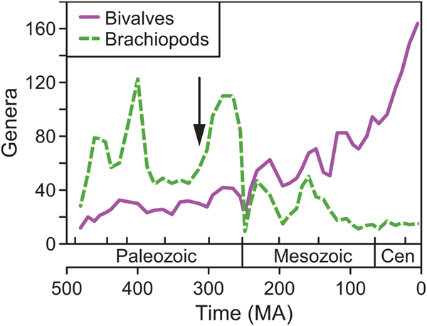
As in previous works (Gould and Calloway Reference Gould and Calloway1980; Miller and Sepkoski Reference Miller and Sepkoski1988), brachiopods were more diverse than bivalves in the Paleozoic, with bivalves becoming more diverse after the Permian extinction (Fig. 1). Bivalves radiated fairly steadily through time (Miller and Sepkoski Reference Miller and Sepkoski1988; Alroy Reference Alroy2010; Foote Reference Foote and Bell2010; Bush et al. Reference Bush, Hunt and Bambach2016), whereas brachiopods declined permanently in the mid-Mesozoic (Sepkoski Reference Sepkoski, Valentine, Jablonski, Erwin and Lipps1996). Notably for this study, bivalve and brachiopod richnesses were fairly similar in the Late Devonian–Carboniferous relative to the rest of the Paleozoic. Thus, one could predict that the ecological importance of bivalves relative to brachiopods might be greater in this time interval than in the rest of the Paleozoic.

Figure 1. Genus richness of brachiopods (dashed line) and bivalves (solid line) from the Ordovician to the Cenozoic based on data from the Paleobiology Database (paleobiodb.org), standardized using shareholder quorum subsampling. Data from Bush et al. (Reference Bush, Hunt and Bambach2016). Arrow marks the approximate temporal position of the Breathitt Formation. Abbreviation: Cen, Cenozoic.
Materials and Methods
Geological and Paleontological Context
The Middle Pennsylvanian Breathitt Formation of eastern Kentucky and neighboring states (Fig. 2A) comprises a number of transgressive marine shales separated by terrestrial strata such as coals (Chesnut Reference Chesnut, Cecil and Eble1989; Bennington Reference Bennington1995). These epicontinental marine units represent repeated flooding events during the late Paleozoic ice age, when Kentucky was located in the tropics, between the equator and 15°S (Scotese and McKerrow Reference Scotese and McKerrow1990). Though there were more brachiopod than bivalve genera overall worldwide, bivalves were already more diverse in some regions, including the Appalachian Basin (Bennington Reference Bennington1995) and parts of southwestern Gondwana (Sterren and Cisterna Reference Sterren and Cisterna2010; Balseiro et al. Reference Balseiro, Sterren and Cisterna2014) .
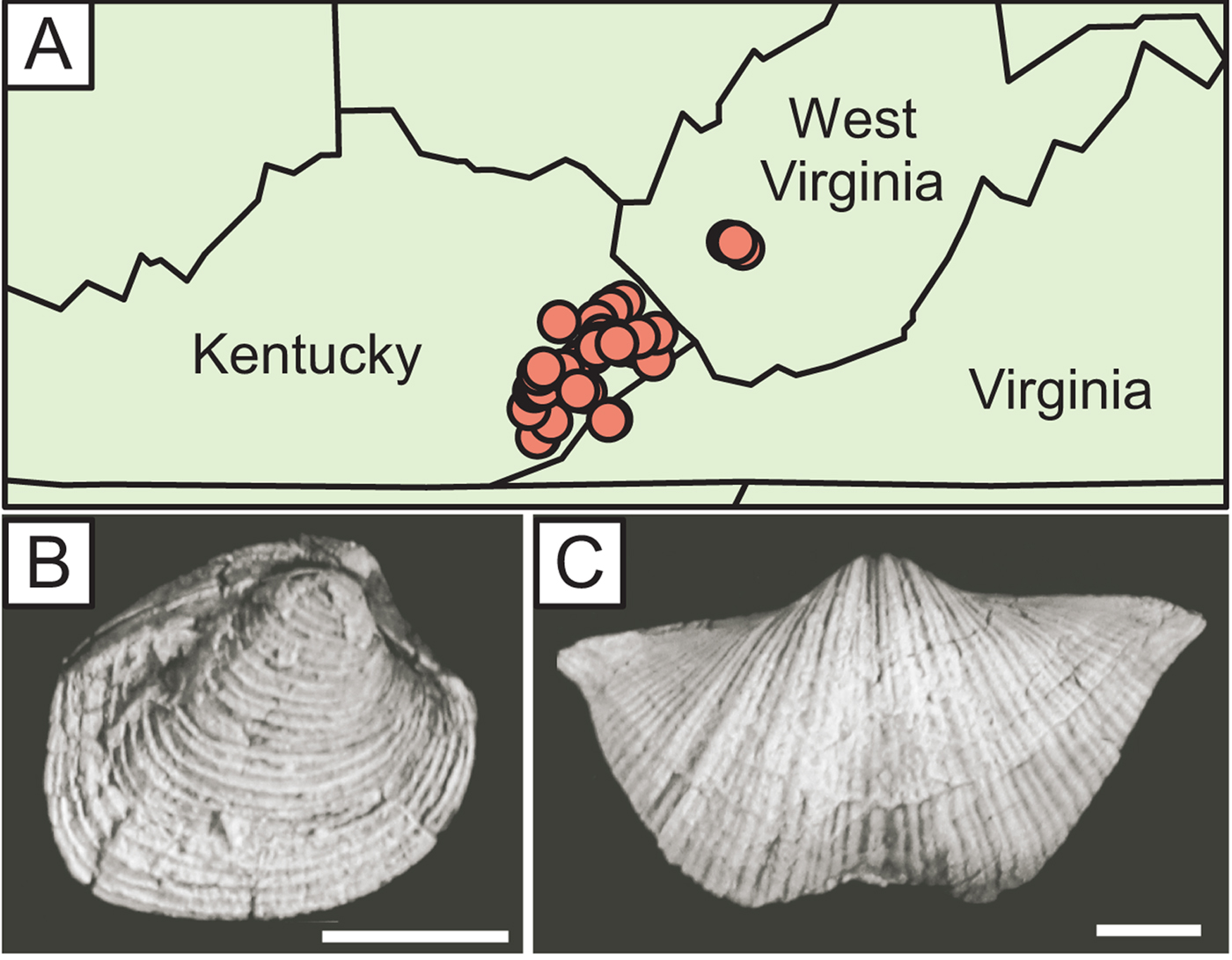
Figure 2. A, Locality map (see Supplementary Table 1 for coordinates). B, Astartella cf. A. compacta, an aragonitic bivalve from the Breathitt Formation. C, Neospirifer cf. N. goreil, a calcitic brachiopod. Scale bars, 5 mm.
For a previous study on community persistence and coordinated stasis in the Breathitt (Bambach and Bennington Reference Bambach, Bennington, Jablonski, Erwin and Lipps1996; Bennington and Bambach Reference Bennington and Bambach1996), Bennington (Reference Bennington1995) tabulated abundances of identifiable fossil taxa from bulk samples (5–10 kg each) collected from the four most extensive marine shale units (Elkins Fork, Kendrick, Magoffin, and Stoney Fork) at 46 localities (Fig. 2A; see Supplementary Tables 1–4 for locality and abundance information). The samples were soaked in detergent and disaggregated carefully by hand under a magnifying lens such that most fossils were separated from the matrix, allaying concerns about the effects of lithification on paleoecological patterns (Hendy Reference Hendy2009; Sessa et al. Reference Sessa, Patzkowsky and Bralower2009). Originally aragonitic shells are preserved as original shell material, not molds (Yochelson et al. Reference Yochelson, White and Gordon1967; Brand Reference Brand1983), and display the same level of fine detail as calcitic shells (Fig. 2B,C), even on small specimens (e.g., 1–2 mm in maximum dimension). The samples are housed at the Virginia Museum of Natural History in Martinsville, Virginia. Twenty-eight species of bivalves and 24 species of brachiopods were identified; other taxa include gastropods, rostroconchs, corals, crinoids, and trilobites, but these were not included in our study. After combining replicate collections from the same horizon at the same locality into single samples, we excluded samples with fewer than 30 specimens, yielding 92 samples and 30,754 specimens. Mean sample size was 334 specimens.
The Breathitt samples represent a range of habitats along a depth gradient in the epicontinental sea. Through cluster analysis, Bambach and Bennington (Reference Bambach, Bennington, Jablonski, Erwin and Lipps1996) and Bennington and Bambach (Reference Bennington and Bambach1996) found that samples generally fell into five paleocommunity types based on species composition and abundance. At one end of the environmental spectrum, a cluster of samples dominated by semi-infaunal productid brachiopods rooted by spines was associated with high-energy, nearshore environments. At the other extreme, the “small mollusk cluster” was dominated by deposit-feeding nuculoid bivalves and occurred in deeper, quieter waters where organic matter could settle. In between were spiriferid, productid–chonetid, and chonetid–mollusk clusters, named after their dominant constituents.
Metrics of Ecological Importance
For each Breathitt sample, we estimated proportional representation of bivalves relative to brachiopods using four metrics that represent different ways of gauging ecological importance: (1) total number of specimens in each clade, (2) shell volume summed across specimens in each clade, (3) biomass summed across specimens in each clade, and (4) energy use summed across specimens in each clade.
To obtain estimates of volume, biomass, and energy use for each species, we measured lengths of the anterior–posterior (AP), dorsal–ventral (DV), and left–right (LR) axes of a subsample of shells to the nearest tenth of a millimeter using digital calipers (Supplementary Tables 5–7). We obtained 4306 measurements from 1677 specimens. For abundant species, we measured 30–60 specimens drawn from numerous samples representing multiple shale units. For rarer species, we measured as many specimens as were available. Many specimens included both valves, but when a bivalve specimen was represented by a single valve, its LR dimension was doubled based on an assumption of symmetry. DV measurements were treated similarly for single valves of equally biconvex brachiopods. All three dimensions could be determined from ventral valves of plano-convex and concavo-convex brachiopods. Due to fragmentation, some specimens were measured in only one or two dimensions. To make use of all available information on size variation (Schafer Reference Schafer1997), the missing data were imputed using the program AMELIA II (Honaker et al. Reference Honaker, King and Blackwell2011) whenever possible. For some species, AMELIA II did not produce a result, so missing values were imputed using the mean ratio of the missing dimension to a more completely known dimension. This method yielded results that were essentially identical to those produced by AMELIA II in species for which both methods could be employed. In calculating volume, biomass, and energy use, each specimen was assigned the average value for its species, which adds some error to individual samples but should cancel out overall.
We modeled volumes of brachiopod and bivalve shells as ellipsoids with volume (4/3)π(x/2)(y/2)(z/2), where x, y, and z are the three measured dimensions for each species, following Finnegan and Droser (Reference Finnegan and Droser2008) (Supplementary Tables 5–7). For biomass, we followed Payne et al. (Reference Payne, Heim, Knope and McClain2014) in calculating ash-free dry mass in grams as 8.0 × 10⁻⁷ × L 3.34 for brachiopods and 1.0 × 10⁻⁵ × L 2.95 for bivalves, where L is the maximum linear dimension of a species (Supplementary Table 5). Chonetid brachiopods are flatter than any of the modern taxa on which these equations are based, so we halved their length before calculating biomass. As in previous paleoecological studies (Finnegan and Droser Reference Finnegan and Droser2008; Finnegan et al. Reference Finnegan, McClain, Kosnik and Payne2011; Payne et al. Reference Payne, Heim, Knope and McClain2014), we calculated average metabolic rate per species using the equation B(M, T) = B 0e −E/kTM 3/4 , where B is the resting metabolic rate in Watts, E is the average activation energy of rate-limiting metabolic reactions, k is Boltzmann's constant, T is the absolute temperature in K, M is body mass, and B 0 is a taxon-dependent scaling constant (Gillooly et al. Reference Gillooly, Brown, West, Savage and Charnov2001).
We assume T is constant within samples, and so e −E/kT is constant within samples and cancels out when calculating within-sample proportions. Proportional metabolic rate depends only on B 0 and M; the values reported in Supplementary Table 5 are thus relative values obtained by arbitrarily setting e −E/kT to 1.0. Following Payne et al. (Reference Payne, Heim, Knope and McClain2014), B 0 equals 6.5 × 10¹⁰ W kg−3/4 for rhynchonelliform brachiopods, 5.6 × 10¹⁰ W kg−3/4 for other brachiopods, 1.4 × 10¹¹ W kg−3/4 for heterodont bivalves, and 1.3 × 10¹¹ W kg−3/4 for non-heterodont bivalves. The difference between brachiopods and bivalves is much greater than the difference between the two groups within each clade, suggesting that the contrast in metabolic rate between bivalves and brachiopods is robust. Individual species doubtlessly varied within each clade, adding additional uncertainty to these analyses, but direct measurements of the metabolic rates of Pennsylvanian species are not available.
Sample-Level Evaluation of Ecological Importance
The proportional representation of bivalves was calculated within each sample using the formula X bivalve/(X bivalve + X brachiopod), where X refers to ecological importance calculated as one of four metrics discussed earlier. Thus, zero indicates complete bivalve dominance, 1.0 indicates complete brachiopod dominance, and 0.5 indicates equal ecological importance (e.g., equal number of specimens, equal biomass). To test the effects of estimating ecological importance without using local abundance data, we calculated all metrics a second time after degrading the data to species occurrences (i.e., every species in a sample treated as having equal abundance). Finally, the four metrics were calculated again using only suspension-feeding bivalves (21 species), which are more ecologically comparable to brachiopods than species that employ other feeding mechanisms.
Regional-Scale Evaluation of Ecological Importance
Each metric was averaged across all samples to obtain an overall estimate of the importance of bivalves relative to brachiopods in the Breathitt. For some treatments, the ecological importance of bivalves was bimodally distributed, with most assemblages containing mostly bivalves or mostly brachiopods. In these cases, the “average assemblage” is a statistical abstraction that resembles few observed assemblages. However, these mean values are intended only to indicate whether, overall, bivalves or brachiopods were more important ecologically. A mathematically equivalent comparison could be made by simply summing bivalve and brachiopod importance across all samples, but with mean values this comparison occurs on the same scale for all metrics. Bimodality does make this calculation more uncertain, which manifests as wider confidence intervals relative to treatments for which the data were unimodally distributed.
In addition, the overall importance of bivalves was evaluated for each metric as the proportion of samples that were “bivalve dominated”—that is, in which the proportional importance of bivalves was greater than 0.50. The 95% confidence intervals around all values were estimated using a two-step resampling routine run at 1000 iterations (individuals in each sample were resampled with replacement, then the 92 samples were resampled with replacement).
Ecological Gradient Analysis
To better understand how bivalves and brachiopods were distributed among the Breathitt samples, thus providing context for our regional-scale results, we performed a nonmetric multidimensional scaling (NMDS) analysis (Minchin Reference Minchin1987; Clarke Reference Clarke1993; Bonelli et al. Reference Bonelli, Brett, Miller and Bennington2006; Tomasovych Reference Tomasovych2006; Bush and Daley Reference Bush, Daley, Kelley and Bambach2008; Bush and Brame Reference Bush and Brame2010). NMDS arranges samples along gradients in species composition that often reflect gradients in environmental parameters; in many cases, the primary axis in ordinations of benthic marine fossils correlates with water depth (Holland et al. Reference Holland, Miller, Meyer and Dattilo2001; Scarponi and Kowalewski Reference Scarponi and Kowalewski2004). We examined the distribution of parameters like shell mineralogy and feeding method within the NMDS ordination to better understand potential controls on bivalve and brachiopod abundance. Abundances were converted to proportions before analysis to account for differences in sample size.
Global-Scale Evaluation of Ecological Importance
Payne et al. (Reference Payne, Heim, Knope and McClain2014) largely analyzed occurrence-level data, but one analysis was based on sample-level abundance counts (Payne et al. Reference Payne, Heim, Knope and McClain2014: Fig. 2b). To complement our regional-scale Breathitt analysis, we performed an updated version of this analysis using Ordovician–Jurassic collections that contained abundance counts for brachiopods and bivalves (downloaded from the PBDB on 18 September 2018). Following Payne et al. (Reference Payne, Heim, Knope and McClain2014), we excluded collections that contained only one of the two taxa, a situation that often reflects the restricted taxonomic focus of the original studies rather than true absences. Furthermore, we excluded collections that had fewer than 30 specimens (bivalves plus brachiopods), the same cutoff used for the Breathitt samples. We calculated the proportional abundance of bivalves in each collection and converted these values to proportional energy use using the body-size data from Payne et al. (Reference Payne, Heim, Knope and McClain2014). Mean values were calculated at the period level, with the exception of the Silurian, for which there were few collections.
Results
Local Scale
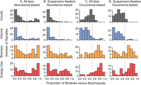
In the primary analysis (all bivalve and brachiopod taxa included, abundance counts used instead of occurrences), the proportional importance of bivalves relative to brachiopods was bimodally distributed for all metrics (Fig. 3A). That is, some samples were bivalve dominated, others were brachiopod dominated, and few contained a relatively even mix. As discussed below, these two modes reflect assemblage types dominated by deposit feeders and by suspension feeders, which occur in different habitats (deeper and shallower, respectively). The bimodal distribution of brachiopod versus bivalve importance is lost for some metrics when considering only suspension feeders, which eliminates many bivalve taxa (Fig. 3B), and when ecological importance is based on the number of occurrences rather than specimens (Fig. 3C,D).

Figure 3. Proportional ecological importance of bivalves relative to brachiopods in bulk samples from the Breathitt Formation, calculated as X bivalve/(X bivalve + X brachiopod), where X refers to one of four measures of ecological importance (number of specimens, shell volume, biomass, and energy use). A value of 0.5 indicates that bivalves and brachiopods are equal for a particular metric; values greater than 0.5 indicate that bivalves are more ecologically important than brachiopods; and values less than 0.5 indicate that bivalves are less ecologically important than brachiopods. A, Weighted by abundance, all species. B, Weighted by abundance, suspension feeders only. C, Weighted by occurrences, all species. D, Weighted by occurrences, suspension feeders only.
The differences between these treatments reflect the different distributions of bivalves and brachiopods with respect to local relative abundance, shell volume, biomass, and energy use (Fig. 4). On average, brachiopods have greater relative abundance per occurrence (Fig. 4A); for example, no bivalve species makes up more than 10% of the specimens in the average sample, whereas several brachiopod species make up more than 15%. Thus, brachiopods appear to be more ecologically important when using abundance data than when using occurrence data. On average, the brachiopod species have slightly more voluminous shells (Fig. 4B), such that brachiopods appear slightly more important using shell volume than using abundance or occurrence counts. Conversely, bivalves tend to have more biomass and higher energy usage (Fig. 4C,D) than brachiopods, such that bivalves have higher ecological importance when these metrics are considered (cf. Payne et al. Reference Payne, Heim, Knope and McClain2014).

Figure 4. Characteristics of bivalve and brachiopod species. A, Mean proportional abundance within samples. B, Estimated shell volume (average value for each species). C, Estimated biomass (average value for each species). D, Estimated relative energy use (average value for each species). Dashed lines mark mean values. Values for B, C, and D are shown on a logarithmic scale. N = 24 for brachiopods and 28 for bivalves.
Regional Scale
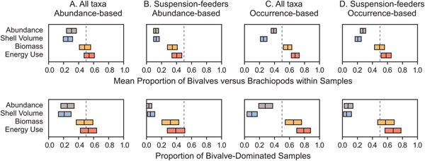
The mean proportional abundance of bivalves (considering only bivalves and brachiopods) in the Breathitt samples was 0.30 (Fig. 5A, top row). For shell volume, biomass, and energy use, the respective values were 0.26, 0.48, and 0.55 (Fig. 5A, top row). The latter two values were not significantly different from 0.50 (i.e., bivalves and brachiopods of equal importance). When only suspension feeders were included, the relative importance of bivalves declined to 0.12 for specimens, 0.12 for shell volume, 0.34 for biomass, and 0.40 for energy use (Fig. 5B, top row), all of which were significantly different from 0.50.

Figure 5. Regional ecological importance of bivalves versus brachiopods in samples from the Breathitt Formation. Top row: the mean proportional ecological importance of bivalves relative to brachiopods in Breathitt samples. Bottom row: the proportion of samples in which bivalves are more important than brachiopods for a given metric. Rectangles indicate 95% confidence intervals. See Fig. 3 for histograms of all sample values. A, Weighted by abundance, all species. B, Weighted by abundance, suspension feeders only. C, Weighted by occurrences, all species. D, Weighted by occurrences, suspension feeders only.
Weighting by occurrences rather than abundances increased the apparent importance of bivalves for almost all metrics (Fig. 5C,D, top row). Bivalves appeared to capture a statistically significant majority of energy use and biomass when all species were considered (Fig. 5C, top row), although biomass was indistinguishable from 0.50 when only suspension feeders were considered (Fig. 5D, top row). These figures were calculated by averaging values calculated separately for each sample, but the results were similar when occurrences for the Breathitt were pooled. Evaluating regional bivalve importance as the proportion of bivalve-dominated assemblages yields generally similar results (Fig. 5, bottom row).
Ecological Gradient Analysis
NMDS axis 1, which captures the greatest amount of variation in species composition among samples, primarily separates Bennington's (Reference Bennington1995) small mollusk cluster (“m” in Fig. 6A) from the brachiopod-dominated clusters (“s,” “c,” and “p”), with the chonetid-mollusk cluster in between (“x”). Indeed, the proportion of brachiopods declines from the negative to the positive end of the axis as the proportion of bivalves increases (Fig. 6C,D). Axis 1 primarily represents a depth-related habitat gradient, as seen in many paleoecological gradient analyses of marine animals (Holland et al. Reference Holland, Miller, Meyer and Dattilo2001; Scarponi and Kowalewski Reference Scarponi and Kowalewski2004). The small mollusk cluster is present in deeper, calmer waters, and the brachiopod-dominated clusters are characteristic of shallower waters (Bennington Reference Bennington1995). The brachiopod-dominated clusters separate along NMDS axis 2 (Fig. 6A).

Figure 6. NMDS ordination of Breathitt samples based on relative abundances of brachiopod and bivalve species. A, Samples labeled by paleocommunity type, as determined by cluster analysis in Bennington and Bambach (Reference Bennington and Bambach1996) and Bambach and Bennington (Reference Bambach, Bennington, Jablonski, Erwin and Lipps1996). B, Samples labeled by stratigraphic unit. C, Proportional abundance of brachiopods. D, Proportional abundance of bivalves. In C and D, point size is scaled continuously between 0.0 and 1.0.
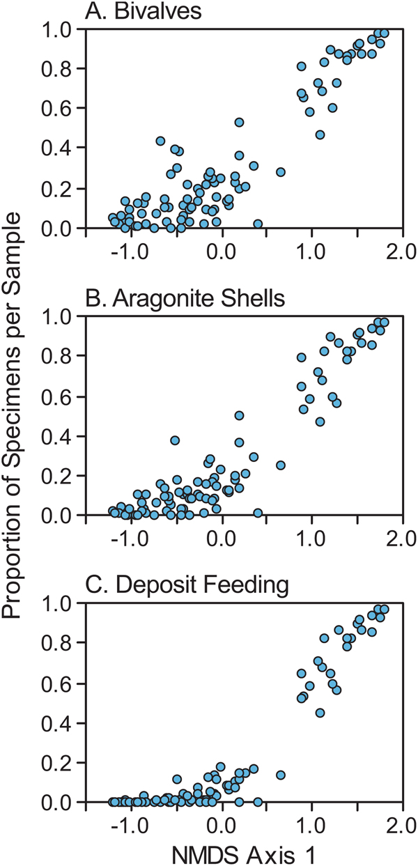
The shift from brachiopod dominance to bivalve dominance along NMDS axis 1 is also illustrated in Figure 7A, in which the position of each sample along axis 1 is plotted against the proportion of bivalves in the sample. The same shift is also reflected in a shift from dominance by calcitic, bimineralic, and phosphatic shells to aragonitic shells (Fig. 7B), and in a shift from suspension feeders to deposit feeders (Fig. 7C). The shift from suspension feeding to deposit feeding along NMDS axis 1 is also apparent when only bivalves are considered (Fig. 8A), because suspension-feeding bivalves tend to co-occur with brachiopods (negative end of axis 1) rather than with their deposit-feeding kin (Fig. 8B,C).

Figure 7. Proportion of specimens in each sample bearing particular traits as a function of position on NMDS axis 1 (Fig. 6). Proportions were calculated relative to the total number of specimens (bivalves plus brachiopods). A, Proportion of bivalves. B, Proportion of aragonite-shelled individuals. C, Proportion of deposit feeders.

Figure 8. Proportion of bivalve specimens in each sample bearing particular traits as a function of position on NMDS axis 1 (Fig. 6). Proportions were calculated relative to the total number of bivalve specimens (i.e., brachiopods were excluded). A, Proportion of deposit feeders. B, Proportion of aragonite-shelled suspension feeders. C, Proportion of bimineralic-shelled suspension feeders.
Global Scale
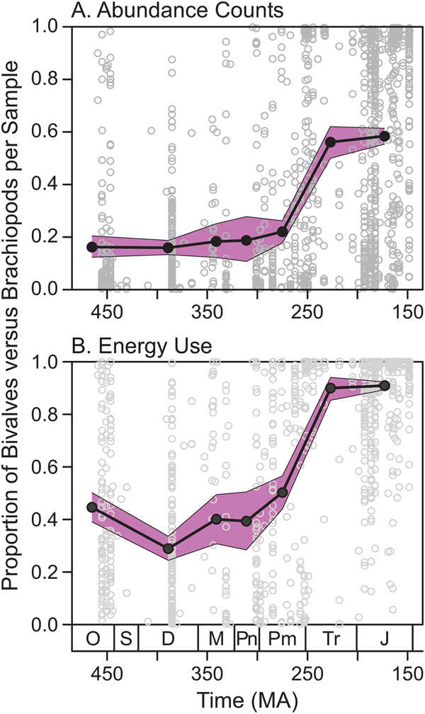
The average proportional abundance of bivalves relative to brachiopods did not change considerably during the Paleozoic; 95% confidence intervals for the Ordovician–Permian overlapped, with mean values ranging between 0.15 and 0.22 (Fig. 9A). Average proportional abundance of bivalves increased sharply from the Permian to the Triassic. The apparent ecological importance of bivalves was higher when considering energy use, with Paleozoic values ranging between 0.28 and 0.50 (Fig. 9B). Again, there was no clear trend from the Ordovician to the Permian, and mean values were much higher in the Triassic and Jurassic (>0.90).

Figure 9. Proportional ecological importance of bivalves versus brachiopods in samples from the Paleobiology Database (paleobiodb.org). A, Proportional abundance within samples. B, Proportional energy use within samples. Gray open circles represent individual collections. Black filled circles represent period-level means, with the Silurian omitted due to small sample size. The shaded bands mark 95% confidence intervals around the means. O, Ordovician; S, Silurian; D, Devonian; M, Mississippian; Pn, Pennsylvanian; Pm, Permian; Tr, Triassic; J, Jurassic.
Discussion
Ecological Importance of Bivalves versus Brachiopods
Local Scale
In the Breathitt ecosystem, bivalves were most common in samples representing deeper-water habitats, and brachiopods were most common in those representing shallower waters (Fig. 6; Bennington Reference Bennington1995). The distribution of abundance was bimodal, with most samples dominated by one clade or the other (Fig. 3A), with the difference largely driven by the profitability of deposit versus suspension feeding (with suspension-feeding bivalves tending to occur with brachiopods) (Figs. 7,8).
Regional Scale
Overall, bivalves and brachiopods were approximately equal in biomass and energy use in the Breathitt ecosystem (indistinguishable from 50%; Fig. 5A), so neither “dominated” in terms of energetics. When only suspension feeders are considered (Fig. 5B), brachiopods used significantly more energy than bivalves (60%; Fig. 5B, top row), suggesting that bivalves held their own against brachiopods by exploiting more feeding mechanisms. (It is worth remembering that our calculations of biomass and energy use are based on extrapolations and simplifications, as were previous similar studies, and should be viewed as rough estimates.)
In other ways, however, brachiopods were clearly more important ecologically than bivalves in the regional fauna. Brachiopods took up more space on the seafloor (i.e., shell volume; Fig. 5A), which could be important, as space can be limiting for benthic animals (Frechette and Lefaivre Reference Frechette and Lefaivre1990), particularly for those species that attach to hard substrates (Taylor and Wilson Reference Taylor and Wilson2003). In addition, shell surface area (values of which would be similar to abundance and volume) is ecologically important, because shelly taxa act as ecosystem engineers by providing hard substrates for other organisms (Sprinkle and Rodgers Reference Sprinkle and Rodgers2010; Rodland et al. Reference Rodland, Simoes, Krause and Kowalewski2014). By modifying habitat availability, an animal can have strong ecological importance as a physical ecosystem engineer, unrelated to its trophic importance (Jones et al. Reference Jones, Lawton and Shachak1994, Reference Jones, Lawton and Shachak1997; Hastings et al. Reference Hastings, Byers, Crooks, Cuddington, Jones, Lambrinos, Talley and Wilson2007). The importance of brachiopods relative to bivalves in providing attachment sites would be enhanced further if their calcitic shells persisted longer in the taphonomically active zone.
Global Scale
Payne et al. (Reference Payne, Heim, Knope and McClain2014: Fig. 2b) showed the average proportional abundance of bivalves within assemblages increasing gradually from the Ordovician to the Jurassic, with no obvious jump across the Permian/Triassic boundary. In contrast, we find that the proportion of bivalves changed little from the Ordovician to the Permian (95% confidence intervals overlap; Fig. 9A), with a sizable jump from the Permian to the Triassic. Likewise, the proportional energy use of bivalves fluctuated during the Paleozoic before rising across the Permian/Triassic boundary (Fig. 9B). These results reinforce the standard view that the Permian–Triassic extinction played a critical role in benthic ecosystem change.
The PBDB results also suggest that the relative ecological importance of bivalves and brachiopods in the Breathitt was not unusual for its time. The average Pennsylvanian sample from the updated PBDB data set contained 19% bivalves by abundance (Fig. 9A), compared with ~40% reported by Payne et al. (Reference Payne, Heim, Knope and McClain2014: Fig. 2b). The Breathitt samples contained 30% bivalves on average, and this value falls to 5% if all taxa with fully aragonitic shells are removed. Thus, the updated PBDB value of 19% for the Pennsylvanian is reasonable if aragonitic specimens are underrepresented in many collections. It is also possible that bivalves are overrepresented in the Breathitt samples relative to other regions—at the global scale, bivalves are less diverse than brachiopods in the Pennsylvanian (Fig. 1), whereas they are actually more diverse in the Breathitt data set. The updated PBDB data suggest that bivalves use 40% of energy on average in the Pennsylvanian (Fig. 9B), compared with ~60–70% in the Payne et al. (Reference Payne, Heim, Knope and McClain2014) data and 54% in the Breathitt samples.
Abundance versus Occurrence Data
In the Breathitt, bivalves used an estimated 67% of energy based on occurrence-level data and 54% based on local abundance counts, with the latter value not significantly different from 50% (Fig. 5A,C). The relative importance of brachiopods was higher using abundance data, because brachiopod species tended to have higher relative abundance than bivalves (Fig. 4A). The same pattern can be seen in the global study of Payne et al. (Reference Payne, Heim, Knope and McClain2014), which found that Pennsylvanian bivalves used ~60–95% of total energy based on occurrence-level data or ~60–70% based on samples with abundance counts.
As noted previously, occurrence-level data are useful in many large-scale studies of diversity and ecology, particularly because collecting abundance counts is time-consuming and impractical for many large-scale studies. However, abundance data provide an important check on occurrence data for the current question. Occurrence-level data will be biased to some degree for this type of study if clades vary in local relative abundance in a systematic way, as is the case here.
Taphonomy and Ecology
Aragonitic shells are unusually well preserved in these samples, but the possibility that some shells were lost must be considered. The most heavily bivalve-dominated samples from the Breathitt contain abundant deposit-feeding protobranchs with aragonitic shells (Fig. 7), and these samples could represent dysoxic to anoxic environments (Bennington Reference Bennington1995) in which aragonite preservation was enhanced (Cherns et al. Reference Cherns, Wheeley and Wright2008; Jordan et al. Reference Jordan, Allison, Hill and Sutton2015). Conceivably, these samples accurately represent the original community composition, whereas brachiopod-dominated samples were altered by aragonite dissolution.
Several lines of evidence suggest that aragonite loss is not a substantial problem. Aragonitic shells are preserved in almost every sample in the data set (88 out of 92, or 96%), arguing against large-scale selective dissolution of the molluscan fauna as a general problem (Bennington Reference Bennington1995: p. 152). However, Bennington (Reference Bennington1995: p. 149) did note that some fossils were preserved as molds in some samples from the Elkins Fork (Fig. 6B), probably as a result of the coarser-grained, more permeable lithology. It is possible that these samples lost additional aragonitic shells that could not be counted, but there is no reason to believe that they were originally mollusk dominated. Bimineralic bivalves, which should be less susceptible to dissolution, were not particularly common in the Elkins Fork samples, making up only 4% of specimens on average. In addition, the mollusk-dominated samples (e.g., small mollusk cluster) had very different brachiopod assemblages from the Elkins Fork samples (productid cluster). Ninety-two percent of the average Elkins Fork brachiopod assemblage consists of Desmoinesia, Juresania, and Linoproductus, whereas these taxa make up only 6% of the brachiopods in the average small mollusk cluster sample. Conversely, 73% of the brachiopods in the average small mollusk cluster sample consist of either chonetids or Crurithyris, which together comprise 0.1% of the average Elkins Fork sample. If the Elkins Fork samples contained a large proportion of mollusks, we would expect to also see brachiopods that live in similar habitats. Although some bivalves might have been lost from these samples, it seems unlikely that they were abundant enough originally that our overall results are affected strongly.
Variations among samples in the abundances of brachiopods and bivalves (Figs. 6C,D and 7A) are easily explained by the ecological strategies and habitat preferences of the taxa: the NMDS axis 1 score is more tightly related to feeding mode (Fig. 7C) than to taxonomy or mineralogy (Fig. 7A,B), and the gap between the two clusters of points is wider and more distinct. In fact, suspension-feeding bivalves—including ones with aragonitic shells—tend to co-occur with suspension-feeding brachiopods at the negative end of NMDS axis 1, not with deposit-feeding bivalves (Fig. 8). Thus, NMDS axis 1 appears to reflect the distribution of feeding types along a depth-related habitat gradient, with taxonomic membership and shell mineralogy correlating with feeding type.
It is possible, of course, that bivalves are somewhat underrepresented in these data, in which case their ecological importance would be somewhat greater than shown in Figure 5. However, there is no indication that the bias is large; if all Elkins Fork samples are excluded, or if all samples that lack aragonitic shells are excluded, the regional proportion of bivalves versus brachiopods shifts by less than 3%.
The numerical dominance of brachiopods contrasts with Cherns and Wright's (Reference Cherns and Wright2000, Reference Cherns and Wright2009) argument that bivalves were likely more abundant than brachiopods in the Paleozoic. However, we note that it is difficult to make accurate quantitative comparisons of bivalve versus brachiopod abundance from silicified assemblages, which can be biased in ways that are not entirely clear (Butts Reference Butts, Laflamme, Schiffbauer and Darroch2014; Clapham Reference Clapham2015; Pruss et al. Reference Pruss, Payne and Westacott2015). These include biases where differences in shell and skeletal composition or structure, and the amount and location of organic matter, may contribute to preferential silicification of some taxa over others. In addition, the silicified and non-silicified faunas in those authors’ comparisons generally contained different sets of taxa, so any differences in bivalve versus brachiopod abundance might be due to habitat preferences, not taphonomy, as argued earlier for the Breathitt.
The exceptional preservation in the Breathitt provides one of the most accurate views of benthic ecology that we are likely to get for the Paleozoic. Our analyses demonstrate that brachiopods are numerically dominant overall and that the two clades are roughly equivalent metabolically. In the Breathitt ecosystem, brachiopods were numerically dominant in habitats where suspension feeding was the most profitable mode of life, whereas bivalves were more numerous where deposit feeding was preferred. The total biomass of each group thus likely depended on the areal extent of each habitat, which probably fluctuated through time, introducing additional uncertainty into attempts to more precisely measure metabolic demands.
Conclusions
Exceptionally preserved fossil assemblages offer valuable opportunities to compare the relative ecological importance of taxa that ordinarily vary in preservation potential. In the Pennsylvanian Breathitt Formation, bivalves with original aragonite shells are preserved alongside brachiopods. A data set consisting of abundance counts and body-size measurements from 92 bulk samples indicates that both clades were ecologically important in the Breathitt ecosystem, although they were most common in different habitats. Neither was clearly dominant over the other in terms of biomass or energy use, although brachiopods were more important in terms of abundance, space usage, and provision of hard substrates for other organisms. Updated global data support the contention that brachiopods were more abundant than bivalves in the Ordovician–Permian, and approximately equivalent in energy use, with major change occurring across the Permian/Triassic boundary.
The ecological importance of brachiopods in many Paleozoic ecosystems contrasts sharply with their insignificance during the late Mesozoic and Cenozoic, reinforcing the critical importance of the Permian and Triassic extinctions and the Mesozoic marine revolution in the evolution of marine benthic ecosystems. However, rather than saying that these events caused a shift from a brachiopod-dominated fauna to a bivalve-dominated fauna, we should say that they caused a shift from a bivalve- and brachiopod-dominated fauna to a bivalve-dominated one.
Acknowledgments
Thanks to J. Caira, L. Park Boush, A. Dooley, L. Ward, the Virginia Museum of Natural History, J. L. Payne, P. R. Getty, G. M. Daley, S. B. Pruss, and R. K. Bambach. Thanks to P. M. Novack-Gottshall and an anonymous reviewer for insightful comments on this article and A. Tomašových and an anonymous reviewer for helpful comments on an earlier draft. In addition, we thank the contributors to the PBDB. This is PBDB contribution number 332.