


Introduction
This paper describes steps towards estimating the frequency of the Earth-like planets around nearby stars, using data from the Kepler mission. The overall approach is to simulate the Kepler's detection process and match the resulting distribution of discovered planets by adjusting the parameters of an assumed underlying distribution function. The resulting best-fit distribution function can then be extrapolated to a range of planet radius and period that may lie outside the range of the underlying data, and in particular the range that includes terrestrial-size planets in the habitable zone.
The topics addressed here are: (1) the working database of exoplanets; (2) additions to the database to fill in missing information; (3) working definitions of Earth-like and Super-Earth planets, and the habitable zone; (4) the empirical noise model; (5) the effect of uncertainty in stellar radii; (6) the minimum detectable radius model; and (7) implications for future estimates of the distribution function as a function of planet radius and period.
Database of exoplanets
The list of exoplanets in this paper is taken from the NASA Exoplanet ArchiveFootnote 1 under the sub-heading ‘browse Kepler Objects of Interest’, and selecting the tab labelled ‘cumulative –active’. The file used here was extracted on 7 May 2014, and contained 7286 row entries. Of these, I deleted entries labelled ‘false positive’ or ‘not dispositioned’, leaving only entries labelled ‘candidate’ or ‘confirmed’. I further deleted 153 entries that had blank values for the star's effective temperature (T eff) or gravity (logg), and another five entries lacking J, H and K magnitudes. For entries where the stellar mass or other parameters were blank, placeholder values of −1 were inserted. The resulting file contains 3511 entries.
For perspective, some of the parameters and ranges of values in the reduced file are as follows: period (0.30–2015 days), planet radius (0.24–115 Earth radii), stellar effective temperature (3089–9578 K), logg (1.87–5.15, cgs), and stellar radius (0.158–19.2 solar radii). For these and other values, some of the extremes may be real outliers, or errors in interpreting the observations. The overwhelming bulk of the entries lie within much tighter ranges. For example, about 98% of the values, where the smallest and largest 1% of entries are ignored, fall in these ranges: period (0.69–484 days), planet radius (0.66–50 Earth radii), effective temperature (3815–6954 K), logg (3.6–4.8) and stellar radius (0.50–3.13 Solar radii). In subsequent analysis steps, the range of parameters is often restricted, either to select a physically meaningful subset (e.g., logg >4.0) or to ensure statistical validity (e.g., planet radius <15 Earth radii); such range restrictions are always carefully noted.
Additions to the database
For some exoplanets in the Archive, the stellar mass is missing, so for statistical completeness I inserted a star mass value derived from the provided values of log and radius. In searching for sources of bias in the data, it might be helpful to have a nominal distance to the target, so for all entries I calculated a distance based on each of the J, H and K magnitudes provided, neglecting interstellar absorption, and averaged the three values to give a single nominal distance to the target. The resulting values range from 24 to 11 130 pc, or ignoring the top and bottom 1% of entries, from 113 to 1673 pc.
Similarly, I calculated Kepler-based absolute magnitudes from Kepler magnitude and distance. The resulting values range from −7.2 to 8.5 or from −2.8 to 4.0 ignoring top and bottom 1% of entries.
Habitable-zone and terrestrial planet definitions
The habitable-zone boundaries have been a controversial topic in recent years. For this paper, I adopt the two habitable-zone definitions proposed by Kopparapu et al. (Reference Kopparapu, Ramirez, Schottelkotte, Kasting, Domagal-Goldman and Eymet2014), and with the authors’ permission I here re-label these as ‘narrow’ and ‘wide’.
The narrow habitable zone is defined as the orbital range between a runaway greenhouse (with hot water vapour) at the inner edge, and a barely sustainable greenhouse (with cold water vapour and CO2) at the outer edge. In the present Solar System, the narrow habitable zone runs from 0.95 to 1.68 au, i.e., encompassing the orbits of the Earth and Mars, but just barely.
The wide habitable zone is defined as an adjustment of the narrow range, based on our understanding of the histories of Venus and Mars. The inner edge is set by the observation that the Venus may have lost its water about 1 Gyr ago when the Sun was 8% fainter. The outer edge is set by the observation that Mars probably had liquid water on its surface some 3.8 Gyr ago when the Sun was 25% fainter. In the present Solar System, this wide habitable zone runs from 0.75 to 1.77 au, i.e., from near Venus at 0.72 au to a bit beyond Mars at 1.52 au.
Kopparapu et al. provide parametric equations for the inner and outer boundaries of the narrow and wide habitable zones in terms of the luminosity and effective temperature of the star, for a range from 2600 to 7200 K, and assuming that an N2 atmosphere is present. The minimum-size habitable zone is claimed to be conservative in the sense that the inner distance could be smaller if variations in relative humidity and clouds were more realistically included, and the outer distance could be larger if additional greenhouse gases (e.g., H2) were present. With these caveats, I calculate the inner and outer habitable-zone boundaries for each planet, using the parametric equation provided by Kopparapu et al.
The definition of a terrestrial planet has been similarly controversial. Early definitions had the radius of a terrestrial planet ranging from 0.5 to 2.0 Earth radii. The lower value was chosen to reflect the fact that Mars, with a radius of 0.53 Earth radii and a mass of 0.11 Earth masses, probably did retain its atmosphere for long enough for life to have been possible there. The upper value was chosen to reflect the fact that the rocky cores of gas giants in the Solar System were believed to be of the order of 10 Earth masses (corresponding to about 2 Earth radii), and that therefore a larger mass planet might end up with a thick atmosphere that would preclude life. For the present paper I adopt the terminology used by the Kepler mission, defining Earth-size to be the range from 0.5 to 1.25 Earth radii, and Super-Earth size to be the range from 1.25 to 2.0 Earth radii.
The radius and period of the Kepler exoplanets are plotted in Fig. 1, where the blue ‘x’ symbols indicate individual planets, solid red circles indicate Earth-size planets in the narrow habitable zone, and open red circles indicate Earth-size and Super-Earth-size planets in the wide habitable zone. All of the habitable-zone planets are candidates (in Kepler terminology), save the one confirmed planet which has a radius of 1.1 Earth radii and a period of 129 days. To guide the eye, the adopted radius boundaries of Neptunes (2–6 Earth radii) and Jupiters (6–15 Earth radii) are indicated as well, again following Kepler mission terminology.

Fig. 1. The radius and period of 3511 Kepler planets, confirmed plus candidates, from the NASA Exoplanet Archive, as described in the text. Planets deemed to be in the narrow habitable zone with Earth-like radii are indicated by solid red circles. Planets in the wide habitable zone with Earth- or Super-Earth radii are indicated by open red circles. The diagonal lines labelled ‘med.F,G’ and ‘med.K’ are the minimum detectable radii of planets for the median properties of each of three groups F, G, K, as determined by effective temperature, assuming an effective SNR of 10 for the ensemble of transits for each planet, per Table 1. Specific detections are expected to scatter above as well as below these median lines. The vertical line at 487 days represents the statistical cutoff in period for a 4-year mission. The planet labels on the right are arbitrary but agree with the category definitions used by the Kepler project.
Noise model
The Kepler mission searches for transiting planets by detecting a transit signal in the form of a decrease in the number of stellar photons collected during a transit. A total of at least three transits are required for most planets; however, in a few cases a two-transit planet is included in the database. The net signal-to-noise ratio (SNR) of the ensemble of transits is required to exceed a threshold, for which Kepler's goal is SNR = 7; however, in practice it may be closer to SNR = 10. The noise in a given transit is the average root-mean-square (rms) fluctuation in detrended time intervals of the same length, outside the transit.
For each star, the ratio of the rms fluctuations to the average number of counts, during standard time intervals of 3, 6 and 12 h, is called the Combined Differential Photometric Precision, or CDPP, expressed in parts per million. The CDPP is discussed by Christiansen et al. (Reference Christiansen, Jenkins, Caldwell, Burke, Tennenbaum, Seader, Thompson, Barclay, Clarke, Li, Smith, Stumpe, Twicken and Van Cleve2012) who show a scatter plot of CDPP6 as a function of Kepler magnitude K p, from which is it clear that there is a strong correlation between CDPP and K p. This correlation suggests that a statistical model of the noise as a function of magnitude might be a useful relationship to investigate.
I downloaded the CDPP values for each target star, in quarters 1 to 8, from the Kepler data siteFootnote 2 at STScI. For each quarter I binned the values in half-magnitude bins from a centre value of K p of 8.5 to 18.0. The number of stars in each bin ranged from about 30 to 31 000, with at least 11 000 stars in each of the six bins from 13.5 to 16.0. The total number averaged about 132 000 stars per quarter. In each magnitude, bin I found the median value of CDPP, for each integration time of 3, 6 and 12 h. These median values were averaged for the 8 quarters, and the rms of the medians taken to be the uncertainty in the average, for each magnitude bin and integration time. These values are shown in Fig. 2, where CDPP (ppm) is plotted as a function of Kepler magnitude. It is clear from the plot that the correlation is very tight, especially in the range from 13.25 to 16.25 where the majority (88%) of the stars lie.

Fig. 2. The median rms noise level of all Kepler stars, as a fraction of the star brightness, expressed as the CDPP for integration times of 3, 6 and 12 h, as a function of Kepler magnitude from 8.25 to 18.25, binned in steps of 0.5 mag. The best-fit lines are drawn through the points, using equation (1) in the text. The best-fit values are used for two purposes: (1) to give a simple relation between the Kepler magnitude and the noise level (on a statistical basis), and (2) to provide a means for estimating the effective dependence of noise on the time, where in practice the time interval of interest is the transit time.
Assuming that the total noise arises from the independent processes of instrument noise and electron counting fluctuations, we have (total noise)2 = (instrument noise)2 + (star noise)2, where the instrument noise is constant for a given integration time, and the star noise is the square root of the number of electrons collected in each given integration time. This equation neglects short-term noise from star spots, for example. For faint stars (13.5 and fainter), the instrument noise dominates. Expanding the noise equation to focus on faint stars, we expect to get a linear relation for the noise as a function of the number of stellar photons. I performed a weighted least-squares fit of the data in Fig. 2, and found the following simple relation for the 6-h CDPP:
 $${\rm CDPP6} = 40.0 + 10^{0.390*{K_{\rm p}}-3.853}{\rm ppm,}$$
which is indicated as a solid black line in Fig. 2. Note that in an ideal photon-noise limited case, the coefficient in the exponent would be 0.4, so it is gratifying that it turns out experimentally to be 0.390, very close to the ideal case. The value of this relation is that it gives a statistical estimate of the noise as a simple function of magnitude. The alternative is to find the average CDPP for each star individually, a viable procedure, but not done here.
The actual distributions of CDPP6 values for the stars in each magnitude bin are shown in Fig. 3. For example, the K p = 14.0 bin is shown as a pink line, with a peak value of about 2700 stars at a median CDPP value of about 75 ppm. The ‘x’ symbols show the values of CDPP for the 10, 25, 50 (median), 75 and 90% points, which are 55, 62, 72, 88 and 112 ppm, respectively. The distributions are relatively sharply peaked, for example the K p = 14.0 curve has half of all its data points within about ±18% of the median.

Fig. 3. The distribution of number of stars in log-spaced bins of noise per star per 6-h interval (CDPP6) is shown, for Kepler magnitudes from 10 to 15. The median value of each colour-coded magnitude is shown by the central ‘+’ sign. The cumulative 10 and 25% points are shown by the ‘+’ signs to the left of the median one, and the 75 and 90% points to the right. The key observation from this plot is that the number of stars of a given magnitude bin is very tightly clustered around a median value of noise, so that in a statistical study the observed magnitude can be used to estimate the noise, and with the use of the time-scaling implied by Fig. 2, the noise can be estimated for any transit time.
The 3-h noise is everywhere greater than the 6-hnoise, and the 6-h noise is likewise everywhere greater than the 12-h noise, as is evident from Fig. 2. If the noise followed the normal model of being white, i.e., a random signal with a constant power spectral density, then we would expect the ratio of CDPP3/CDPP6 to be 21/2 or 1.414, and likewise for CDPP6/CDPP12. However, the actual ratios are smaller, indicating the presence of low-frequency or so-called 1/f noise. Taking the mean of ratios of CDPP values in the magnitude range 12–16, I find that the noise varies with integration time as
 $${\rm CDPP}(t)/{\rm CDPP6} = (t/6)^{-x},$$
where
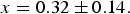 $$x = 0.32 \pm 0.14. $$
This is the time dependence to be used in estimating the noise for transits that take t hours.
Stellar radius bias and uncertainty
A fractional error (ΔR s/R s) in the adopted stellar radius, with respect to the true value, leads directly to an identical fractional error in the estimated planet radius, via the simple area-blocking effect of the transit event. A stellar radius error also leads, nearly linearly, to an error in the estimated minimum detectable planet radius (see the following section, equation (5)). So for the purpose of estimating the completeness of the Kepler sample at a given period, these two effects tend to bias the data in similar ways, and therefore may be expected to have a minimal effect on the final estimate of eta-Earth.
One estimate of the fractional radius error in the Kepler catalogue is provided by Verner et al. (Reference Verner2011), who measured over 500 Solar-type stars in the Kepler catalogue using asteroseismology, and compared the derived radii with Kepler catalogue values. Judging from visual inspection of Fig. 4 in their paper, for stars in the nominal range from about 1 to 2 Solar radii, the Keck catalogue values tend to be about 0.8 ± 0.2 times as large as the seismology radii, where the indicated uncertainty suggests the scatter in values. We assume that the true radii are close to the seismology radii. If this is applied as a correction factor to all catalogue stars, the resulting planet radii would all be a factor of 1/0.8 or about 25% larger than presently estimated.
A second estimate of the accuracy of the Kepler stellar radii is found in Huber et al. (Reference Huber2014), Fig. 11, where a comparison of radii from detached eclipsing binary systems is used to calibrate values of effective temperature, gravity, and metals abundance, which in turn are used to estimate radii. This comparison shows a very tight correlation of Kepler radii with the calibration radii, with the Kepler radii tending to be about 5% smaller, in agreement with the sign of bias in Verner et al. (Reference Verner2011).
A third estimate of the fractional radius error in the Kepler catalogue comes from Farmer et al. (Reference Farmer, Kolb and Norton2013), who use population synthesis tools to create a synthetic catalogue, which they then compare to the Kepler catalogue. They find that the Kepler radii are larger than their synthetic radii by a factor of about 1.03, which is in the opposite direction of the result from the above two studies. Of course this result would imply that we should reduce all derived planet radii by about 3%.
The resulting uncertainty in these bias estimates suggests that we should take no action at present to make wholesale adjustments to the stellar radius values in the Kepler catalogue. Although if we take the asteroseismology and eclipsing binary results at face value, it does suggest that ultimately the derived planet radii will have to be increased by something similar to the 5–25% values found above.
Minimum detectable radius
The SNR for detecting multiple transits of a planet is the ratio of the number of electrons in a single transit divided by the noise during the time of transit, multiplied by the square root of the number of transits (assuming a square-root law for widely separated transits). This ratio is to be set equal to the minimum acceptable SNR in the search algorithm, nominally SNR = 7, but in practice effectively suspected to be roughly SNR = 10. Assuming circular orbits, and Kepler's law relating period and semi-major axis, the result can be expressed as a minimum detectable planet radius, r p (min), in terms of measurable values of CDPP6 (ppm), SNR, period P (days), stellar radius r s (Solar radii), stellar logg (cgs units), duty cycle f 0 (here estimated to be about 0.92), total observing time T (years) and the time exponent of the noise x (specified above).
The resulting relation for the minimum detectable planet radius is
 $${r_{\rm p}}({\rm min})/{r_{\rm Earth}} = 0.017 \times {({\rm CDPP6} \times {\rm SNR})^{1/2}} \times {P^{(1/4 - x/6)}} \times {({r_{\rm s}}/{r_{\rm sun}})^{(1 - x/6)}} \times 10^{(x/6){\rm logg}} \times {({\,f_0}T)^{-1/4}}.$$
Inserting the value x = 0.32, we find
 $${r_{\rm p}}({\rm min})/{r_{{\rm Earth}}} = 0.017 \times {({\rm CDPP6} \times {\rm SNR})^{1/2}} \times {P^{0.197}} \times {({r_{\rm s}}/{r_{{\rm sun}}})^{0.947}} \times 10^{0.053{\rm logg}} \times {({\,f_0}T)^{-1/4}}.$$
It is of interest to see how this relation compares to the scatter diagram of planet radii in Fig. 1. For a first-order look, I split the list of 3511 planets into three equal groups, and found the median values of effective temperature, Kepler magnitude, stellar radius and logg in each group, listed in Table 1. The magnitude gives a noise value (CDPP6). The temperature gives a nominal spectral type (Gray Reference Gray2005, appendix B), for reference. For SNR = 10 and a mission length of T = 4 years, the resulting values of the minimum detectable planet radius are listed in the Table. Given that the median parameter values vary significantly between groups, it is surprising that the minimum detectable radius values turn out to be so similar in value.
Table 1. Median values of stars in each of three groups as defined by the effective temperature

For each group, the minimum detectable planet radius, for an assumed effective SNR of 10, as a function of planet period only, is given in the right-most column, where the period P is in days.
The minimum detectable planet radius given in Table 1 is a statistically determined estimate for each of the three effective temperature groups. As individual stars deviate from the median in each of their properties, so should the observed data be expected to scatter around the mean curve. The r p (min) values are plotted in Fig. 1, where it is seen that the median line does indeed appear to follow the trend of the lower range of radii at all periods. This agreement confirms what is widely believed to be the case, that the fall-off in numbers of planets at small radii is an artefact of the limitation of the stellar signal strength (i.e., number of detected photons) and not necessarily a reflection of the underlying population.
The minimum-radius lines in Fig. 1 terminate at P = 487 days, because this is the statistically expected limit of measurement of Kepler given its nominal 4-year (16 quarters) lifetime. Note that this limit is not a hard cutoff, because some planets will have their transits phased so that three longer-period values can be detected, and some fewer. In addition, some of the detected planets have had only two transits, as the database used here includes these types as well.
Summary
This paper provides several of the beginning steps that can lead to an analysis of the Kepler data based on a forward simulation of the operation of the instrument, with the ultimate goal of applying this simulation to a variety of underlying population distribution functions, and with the expectation of being able to simulate the observed sample of planets.
The purpose of having a minimally biased estimate of the distribution function of the population is several fold. (1) The distribution could give us clues as to the origin and history of planetary systems. (2) The distribution could allow us to compare with planets found by other techniques, with a goal of eventually reconciling all techniques within a common framework. (3) The distribution will help us predict the yield of future transit-measuring missions. (4) The distribution could give us a tool to use for extrapolating to longer-period gas- and ice-giant planets that might be directly imaged by a future direct-imaging mission. (5) And the distribution could be extrapolated to the longer periods and smaller radii of the terrestrial habitable-zone population, which will be needed for future terrestrial planet finder and follow-up missions.
Acknowledgements
This research has made use of the NASA Exoplanet Archive, which is operated by the California Institute of Technology, under contract with the National Aeronautics and Space Administration under the Exoplanet Exploration Programme. Some of the data presented in this paper were obtained from the Mikulski Archive for Space Telescopes (MAST). STScI is operated by the Association of Universities for Research in Astronomy, Inc., under NASA contract NAS5-26555. Support for MAST for non-HST data is provided by the NASA Office of Space Science via grant NNX13AC07G and by other grants and contracts. This paper includes data collected by the Kepler mission. Funding for the Kepler mission is provided by the NASA Science Mission directorate. Copyright 2014, California Institute of Technology.


