


1. INTRODUCTION
When operating in restricted water and forced to deviate from the centre of the channel under vessel meeting and passing conditions, a ship inevitably approaches the bank and thus an asymmetric flow pattern is produced which generates a pressure difference between the port and starboard sides of the vessel. Generally speaking, a suction effect is induced toward the stern of the vessel, while a cushioning effect is induced at the bow. Thus, as shown in Figure 1, the vessel experiences a positive yaw moment, Nb, which pushes the bow toward the centre of the channel and a lateral sway force, Yb, which is directed principally toward the nearest bank. This phenomenon is known as the bank effect and depends on many parameters, including the vessel speed, the distance to bank, the propeller speed, the water depth, the shape of the bank, and so forth. The bank effect has a significant impact on the manoeuvring characteristics of the vessel and must therefore be taken into account when navigating the vessel through the restricted waterway.

Figure 1. Forces acting on ship when navigating in close proximity to lateral bank.
While the validity of the mathematical models embodied in the Standards for Ship Manoeuvrability International Maritime Organization (IMO) in 2002 is generally accepted for assessing the adequacy of manoeuvrability in deep, unrestricted waters at sea speed, their suitability for predicting the effects of the ship-bank interaction when navigating in narrow waterways is subject to considerable doubt. However, due to prohibitive costs, very few ship trials have been performed in shallow water, and the resulting lack of experimental data seriously limits the ability of existing ship-handling simulators to accurately reproduce the yaw and sway motions experienced by a vessel when operating in close vicinity to a bank (Alexander Reference Alexander2005). Nonetheless, as the rate at which the dimensions of many types of ships continues to outstrip that at which the dimensions of the access channels, rivers and ports frequented by these vessels are enlarged, the need for more realistic prediction methods for enhancing the capabilities of ship-handling simulators is emerging as a major concern in the maritime community (Lataire et al. Reference Lataire, Vantorre, Laforce, Eloot and Delefortrie2006).
Due to the expense of conducting real-ship experiments under realistic shallow-water conditions, most previous investigations into the bank effect have taken the form of ship model tests performed in a towing tank. Norrbin (Reference Norrbin1974) investigated the forces acting on a ship in a short dredged channel and found that the bank effect had a significant impact upon the hydrodynamic force coefficient of the vessel. Ch'ng (Reference Ch'ng1991) and Ch'ng and Renilson (Reference Ch'ng and Renilson1993) showed that the magnitude and direction of the yaw angle and sway force experienced by a vessel operating in restricted water are highly sensitive to variations in the hull form, the vessel speed, the distance to bank, the slope of the bank and the propeller speed for values of the water-depth-to-draught ratio of less than 1·5. Li (Reference Li2000) conducted a series of experimental trials to investigate the bank effects exerted on three different ship models under extreme shallow water and near-bank conditions. The results showed that at water-depth-to-draught ratios of less than approximately 1·1, the sway force changed from a suction force to a repulsion force and a significant increase occurred in both the sway force and the yaw moment as a result of the significant magnification of the Bernoulli wave effect. Utilizing two bulk carrier models from the MarAd series and the S175 containership, Duffy (Reference Duffy2002) performed a series of model scale experiments to clarify the respective effects of the water depth, ship draught, bank height, bank slope and the distance to bank on the resultant sway force and yaw moment. The results of a regression analysis showed that both the sway force and the yaw moment were linearly related to the distance-to-bank parameter. Lataire et al. (Reference Lataire, Vantorre, Laforce, Eloot and Delefortrie2006) performed towing tests in the Towing Tank for Manoeuvres in Shallow Water at the Flanders Hydraulic Research Centre in Ghent University, Belgium, using three models, namely an 8000 TEU container carrier, a 131,235 m3 LNG carrier and a small tanker. The experiments were aimed predominantly at clarifying the effects of the bank geometry on the magnitude of the bank effects induced on vessels with different hull forms, speeds, propulsion forces, drift angles, distances to bank, and so forth. Overall, the results demonstrated that an inverse correlation existed between the ship-to-bank distance and the magnitudes of the sway force and yaw moment, respectively.
With rapid advances in the speed and computational capabilities of mainstream computers in recent decades, the use of computational fluid dynamics (CFD) simulations as a means of predicting the hydrodynamic forces acting on a vessel under a wide range of environmental and operating conditions has attracted considerable interest in the maritime community. For example, Xiong and Wu (Reference Xiong and Wu1996) applied the Rankine source method to investigate the hydrodynamic forces acting on the hull of a ship with a free surface effect whilst in restricted water. Ohmori (Reference Ohmori1998) and Berth et al. (Reference Berth, Bigot and Laurens1998) performed Finite Volume Method (FVM) simulations and FLUENT CFD simulations, respectively, based on the Navier-Stokes equation to model the viscous flow field and hydrodynamic characteristics of the ESSO OSAKA oil tanker while advancing and turning in shallow waters. Chen et al. (Reference Chen, Lin and Hwang2002; Reference Chen, Lin, Liut and Hwang2003) utilized the chimera RANS method to examine the problem of ship-to-ship interactions in shallow water and restricted waterways.
In general, the results of the CFD studies discussed above confirm the validity of the CFD approach as a means of obtaining detailed insights into the bank effects acting on vessels operating in restricted water. Accordingly, this study conducts a series of simulations using the commercial FLOW-3D® software package to investigate the ship-bank interaction effect for a Post-Panamax container ship advancing at a constant speed in a direction parallel to that of a lateral bank. The simulations focus specifically on the respective effects of the ship speed and distance-to-bank parameter on the time-based variation of the magnitude and direction of the yaw moment and sway force. In addition, the bank effect phenomena are clarified by reference to visualization plots showing the evolution over time of the pressure and velocity distributions in the immediate vicinity of the vessel. Overall, the results presented in this study contribute a further understanding of the bank effect and yield a useful set of guidelines suitable for implementation into ship-handling simulators designed to predict the response of a vessel under near-bank conditions.
2. NAVIER-STOKES EQUATIONS
In the FLOW-3D® CFD simulations performed in this study, the motion of the water surrounding the ship is modelled using the Navier-Stokes equations. Given an orthogonal coordinate system, the Navier-Stokes continuity equation has the form
while the momentum equation is given by
where ![]() denotes the velocity component in the x-, y- or z-direction, respectively, P is the pressure, ρ and ν are the density and viscosity coefficient of the fluid, respectively, and g is the gravitational force. Note that in performing the simulations, all the parameters in Equations (1) and (2) other than the ship velocity are assumed to be constant.
denotes the velocity component in the x-, y- or z-direction, respectively, P is the pressure, ρ and ν are the density and viscosity coefficient of the fluid, respectively, and g is the gravitational force. Note that in performing the simulations, all the parameters in Equations (1) and (2) other than the ship velocity are assumed to be constant.
3. NUMERICAL SIMULATION PROCEDURE
3.1. Establish ship model
The simulations performed in this study utilize the KRISO (Korea Research Institute of Ships and Ocean Engineering) 3600 TEU Post-Panamax Container Ship (KCS) model. The major parameters and dimensions of both the simulation model and the actual vessel are summarized in Table 1.
Table 1. Parameters of real ship and KCS 3600 TEU model.

3.2. Establish test velocity
As shown in Table 1, the real container ship has a length between perpendiculars of L pp=230 m, and the model scaling ratio is given by λ=Ls/Lm=31·5994. Assuming the velocity of the real ship to be denoted as Vs, the equivalent ship model velocity, Vm, was computed in accordance with the following procedure.
In general, the Reynolds number, Re, is given by the ratio of the inertia force to the viscous force, i.e.
where V is the characteristic velocity (m/s), L is the characteristic length (m) and v is the kinematic viscosity (m 2/s). Utilizing the Reynolds number as a similarity parameter to ensure the appropriateness of the modelling results, the following condition should hold:
Rearranging, it can be shown that

Furthermore, assuming the Froude number, Fr, of the ship model to be equivalent to that of the real ship, it follows that
Rearranging Equation (6) and introducing the ship length parameter values from Table 1, it can be shown that the ship model velocity is given by

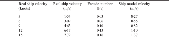
Obviously ![]() , and thus the conditions (Fr)m=(Fr)s and (Re)m=(Re)s can not be satisfied simultaneously. In other words, the model velocity obtained by assuming a similarity of the Reynolds number differs from that obtained by assuming an equivalent Froude number. In a typical ship model experiment, the characteristic Reynolds number is generally of the order of 106~107, while that for a real ship is usually of the order of 108~109 since the viscous force is much lower relative to the developed inertia force. Since the Froude number, Fr, and Reynolds number, Re, of the real ship cannot be equal to the Reynolds number, Re, and Froude number, Fr, of the ship model, respectively, it is simplest for the sake of expediency to neglect the viscous force consideration and to calculate the model velocity based on the Froude equivalency condition. (Note that any errors arising as a result of the corresponding inequality of the Reynolds number can be corrected at a later date based upon experience.) Table 2 compares the real ship velocities and simulation velocities considered in the present study. As shown, the real ship velocities are assumed to be 3, 6, 9, 12 and 15 knots, respectively, corresponding to velocities of 1·54 m/s, 3·09 m/s, 4·63 m/s, 6·17 m/s, and 7·72 m/s, respectively. The equivalent Froude numbers are 0·03, 0·06, 0·10, 0·13 and 0·16, respectively, and thus the ship model velocities are determined to be 0·27 m/s, 0·55 m/s, 0·82 m/s, 1·10 m/s, and 1·37 m/s, respectively.
, and thus the conditions (Fr)m=(Fr)s and (Re)m=(Re)s can not be satisfied simultaneously. In other words, the model velocity obtained by assuming a similarity of the Reynolds number differs from that obtained by assuming an equivalent Froude number. In a typical ship model experiment, the characteristic Reynolds number is generally of the order of 106~107, while that for a real ship is usually of the order of 108~109 since the viscous force is much lower relative to the developed inertia force. Since the Froude number, Fr, and Reynolds number, Re, of the real ship cannot be equal to the Reynolds number, Re, and Froude number, Fr, of the ship model, respectively, it is simplest for the sake of expediency to neglect the viscous force consideration and to calculate the model velocity based on the Froude equivalency condition. (Note that any errors arising as a result of the corresponding inequality of the Reynolds number can be corrected at a later date based upon experience.) Table 2 compares the real ship velocities and simulation velocities considered in the present study. As shown, the real ship velocities are assumed to be 3, 6, 9, 12 and 15 knots, respectively, corresponding to velocities of 1·54 m/s, 3·09 m/s, 4·63 m/s, 6·17 m/s, and 7·72 m/s, respectively. The equivalent Froude numbers are 0·03, 0·06, 0·10, 0·13 and 0·16, respectively, and thus the ship model velocities are determined to be 0·27 m/s, 0·55 m/s, 0·82 m/s, 1·10 m/s, and 1·37 m/s, respectively.
Table 2. Comparison of real ship velocity and KCS 3600 TEU model velocity.
3.3. Establish numerical model of waterway
Figure 2 presents a schematic illustration showing the cross-section of the waterway model used in the CFD simulations. Note that in this figure, h is the water depth, T is the draught of the ship model, B is the beam of the ship model, UKC is the under keel clearance, d2b is the distance to bank, and Y/B is the width of the waterway. In general, the correlation between the draught of a ship, the under keel clearance and the water depth is expressed by the ratio h/T (ITTC 2002) and generally varies in the range 1·1~1·5 for most large ports (Ch'ng Reference Ch'ng1991; Ch'ng and Renilson Reference Ch'ng and Renilson1993; Li Reference Li2000). In the present simulations, the water depth is specified as 14·2 m; corresponding to the low-tide depth of the navigation channel in Kaoshiung port in southern Taiwan. As shown in Table 1, the draught of the real Post-Panamax container ship is 10·8 m, and thus the water-depth-to-draught ratio has a value of h/T=1·31. To prevent the accuracy of the simulation results for the ship-bank interactions from being affected by the waves reflected from the far bank, the width of the waterway model was specified as eight times the beam of the ship in accordance with the recommendations of the International Towing Tank Conference (ITTC, 2005). Moreover, the length of the waterway was specified as 11B, 14B, 17B, 19B or 22B for ship model velocities of 0·27m/s, 0·55m/s, 0·82m/s, 1·10m/s and 1·37m/s, respectively. Following a comprehensive grid-dependency test, it was determined that the optimal waterway model comprised a total of approximately 3 million individual grids.

Figure 2. Cross-sectional view of numerical waterway model.
The simulations performed in this study solve the ship-fluid coupled motion equation (Wei Reference Wei2005) and utilize two orthogonal coordinate systems, namely a body-fixed system and an earth-fixed system (Baha Reference Baha2000). As shown in Figure 3, the body-fixed system (x′y′z′) is attached to the ship model, while the earth-fixed system (x y z ) is attached to the waterway model. In the simulations, an assumption is made that at time t=0, the ship is located at the origin of the waterway framework with the (x′y′z′) axes of the ship coordinate system parallel to the corresponding axes of the waterway model. As time elapses, the ship model advances at the specified velocity along the x-axis (i.e. along a direction heading of 090o) and the velocity flow field and pressure distribution in the immediate vicinity of the ship are computed at each time step. As the ship advances, it performs a three degree-of-freedom (3-DOF) motion relative to the (x, y, z) axes of the waterway model, namely “surge”, i.e. a displacement of the ship along the x-axis, “sway”, i.e. a displacement of the ship along the y-axis, and “heave”, i.e. a displacement of the ship along the z-axis. The ship simultaneously performs a 3-DOF motion about its own coordinate framework, namely “roll”, i.e. a rotation about the x′-axis, “pitch”, i.e. a rotation about the y′-axis, and “yaw”, i.e. a rotation about the z′-axis. Thus, the motion of the ship model has potentially six degrees of freedom (6-DOF).

Figure 3. Schematic view of numerical waterway model.
4. RESULTS AND DISCUSSION
4.1. Validation of simulation model
Prior to performing the bank effect simulations, the validity of the FLOW-3D® simulation model was confirmed by computing the hydrodynamic resistance acting on a small boat with a length of 3·0 m, a beam of 0·8 m, a draught of 0·2 m and a mass of 118·2 kg as it travelled along the x-axis of the waterway model. The mass centre inertia tensor of the boat is given by
![{\rm I} \equals \left[ {\matrix{ {6\hskip-1pt\cdot\hskip-1pt 7} \hfill \tab {0\hskip-1pt\cdot\hskip-1pt 0} \hfill \tab {0\hskip-1pt\cdot\hskip-1pt 0} \hfill \cr {0\hskip-1pt\cdot\hskip-1pt 0} \hfill \tab {93\hskip-1pt\cdot\hskip-1pt 0} \hfill \tab {0\hskip-1pt\cdot\hskip-1pt 0} \hfill \cr {0\hskip-1pt\cdot\hskip-1pt 0} \hfill \tab {0\hskip-1pt\cdot\hskip-1pt 0} \hfill \tab {96\hskip-1pt\cdot\hskip-1pt 7} \hfill \cr} } \right]\lpar {\rm m}^{\setnum{2}} \cdot {\rm kg}\rpar](https://static.cambridge.org/binary/version/id/urn:cambridge.org:id:binary:20151022094657197-0601:S037346330900527X_eqn8.gif?pub-status=live)
In the validation simulations, the calculation area comprised a total of 156,388 grids and the solution was obtained using the implicit Successive Over-Relaxation (SOR) scheme with the FLOW-3D® Renormalized Group (RNG) turbulence model and General Moving Objects (GMO) model. The simulations considered boat speeds of 5·04 m/s, 5·88 m/s, 6·72 m/s, and 7·98 m/s, respectively, and had a duration of t=4s in every case. The calculated values of the hydrodynamic resistance acting on the boat at each speed are summarized in Table 3. Note that the resistance values presented for speeds of 5·04 m/s, 5·88 m/s and 6·72 m/s, respectively, denote the average value obtained over the last 1 second of the simulation, while that presented for a velocity of 7·98 m/s is the average value computed over the interval t=2·2~4·0s. For comparison purposes, the table also presents the resistance values reported by Azimut Yachts for a vessel of a similar size. It is observed that a good agreement exists between the two sets of results at each value of the boat speed, and thus the basic validity of the simulation model is confirmed.
Table 3. Comparison of FLOW-3D® hydrodynamic resistance calculations and shipyard resistance measurements (Wei Reference Wei2006)
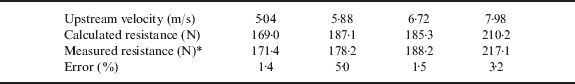
* Data reproduced courtesy of Azimut Yachts.
4.2. Analysis of ship trajectory
The simulations commenced by modelling the trajectory of the KCS model over a duration of 12 seconds as it advanced in the eastward direction at a constant speed of 0·27 m/s, 0·55 m/s, 0·82 m/s, 1·10 m/s and 1·37 m/s, respectively. Figure 4 illustrates the trajectories of the KCS model when advancing at a speed of 0·82 m/s at various distances from the bank. Note that in each case, the trajectories are obtained simply by overlaying the positions of the boat after elapsed times of t=0s, t=2s, t=4s, t=6s, t=8s, t=10s, and t=12s, respectively. In every sub-figure, the x-axis (X/B) indicates the displacement of the ship model in the eastward direction, while the y-axis (Y/B) represents the perpendicular distance between the mass centre of the ship model and the bank. Meanwhile, the caption beneath each sub-figure indicates the yaw angle of the ship model upon completion of the simulation (i.e. t=12s). The simulation results clearly show that for a constant ship speed, the yaw angle increases as the distance between the ship and the bank reduces. From inspection, the final yaw angle for an initial ship-to-bank distance of 0·5B is determined to be 12 times higher than that of the final yaw angle for an initial ship-to-bank distance of 3·0B.

Figure 4. Ship trajectories whilst navigating at Vm=0·82 m/s with d2b=0·5~3·0B.
4.3. Analysis of yaw angle and yaw velocity
Figure 5 illustrates the correlation between the distance to bank, the ship speed and the yaw degree. The results confirm that for a constant ship velocity, the yaw angle increases significantly with a reducing distance to bank. In addition, it is observed that the sensitivity of the yaw angle to the distance-to-bank parameter is particularly pronounced at higher values of the ship speed. The results also show that for a given value of the distance-to-bank parameter, the yaw angle increases with an increasing velocity; particularly at lower values of the ship-to-bank distance.

Figure 5. Correlation between distance to bank, ship speed and yaw angle.
Since the ship model potentially performs a 6-DOF motion, the bow may rotate about the z-axis at the same time as the ship advances along the x-axis. According to the right-hand law, a positive value of the angular yaw velocity indicates a counterclockwise rotation of the bow, i.e. the bow moves in the port direction and the heading angle reduces. Conversely, a negative value of the angular yaw velocity indicates that the bow rotates in the clockwise direction, i.e. the bow moves in the starboard direction and the heading angle increases. Figures 6(a) and 6(b) illustrate the time-based variation of the yaw velocity as a function of the ship model speed for distance-to-bank values of 0·5B and 3·0B, respectively. Figure 6(a) shows that at a low value of the ship-to-bank distance, the yaw velocity has a consistently positive value at virtually all values of the ship speed, which indicates that the bow rotates in the counterclockwise direction, i.e. away from the bank. Furthermore, it can be seen that the magnitude of the yaw velocity is significantly dependent upon the ship speed, and increases with an increasing velocity. For the case of a higher ship-to-bank distance, the results presented in Figure 6(b) indicate that for a constant velocity, the bow of the ship tends to oscillate between the port and starboard directions as the ship advances. Furthermore, it is evident that the magnitude of the yaw velocity is relatively insensitive to the ship speed. Overall, therefore, the results suggest that the bank effect diminishes as the distance between the ship and the bank increases.

Figure 6. Time-based variation of yaw moment as function of ship speed for: (a) d2b=0·5B and (b) d2b=3·0B.
4.4. Analysis of sway force
Figures 7(a) and 7(b) illustrate the time-based variation of the sway force as a function of the ship speed at distance-to-bank values of 0·5B and 3·0B, respectively. Comparing the two figures, it is evident that the sway force is dominated by the distance-to-bank parameter, whereas the ship speed has a relatively lesser effect. Furthermore, it is seen that the individual sway force profiles have a relatively uniform oscillatory characteristic with a period of approximately 2 seconds. An increasing value of the sway force indicates that the flow field between the ship and the bank forces the ship toward the centre of the channel, whilst a decreasing value of the sway force indicates that the flow field pulls the ship toward the bank. The two figures show that the bank effect is first manifested after an elapsed simulation time of approximately 3 seconds, i.e. the sway force adopts a negative value, which indicates that the stern of the ship approaches the bank as a result of the yaw rotation of the bow in the port direction (see Figure 6).

Figure 7. Time-based variation of sway force as function of ship speed for: (a) d2b=0·5B and (b) d2b=3·0B.
Figure 8 illustrates the correlation between the distance to bank, the ship speed and the sway force. In general, the results show that for a constant value of the ship-to-bank distance, the sway force increases with an increasing velocity. The sensitivity of the sway force to variations in the ship speed is particularly pronounced at low values of the ship-to-bank distance. Meanwhile, for a constant value of the ship speed, the sway force increases with a reducing ship-to-bank distance. The sensitivity of the sway force to changes in the ship-to-bank distance is particularly apparent at higher values of the ship speed.

Figure 8. Correlation between distance to bank, ship speed and sway force.
4.5. Analysis of flow field pressure distribution at Vm=0·82m/s
Figures 9(a~b) and 9(c~d) illustrate the time-based evolution of the pressure distribution on the x-y plane located at a depth of −0·06 (Z/B) for distance-to-bank values of 0·5B and 3·0B, respectively. Note that the ship speed is 0·82 m/s in both cases. Comparing the two figures, it is observed that the pressure distribution around the ship model is far more uniform in the case of the higher ship-to-bank distance, and thus no more than a minor yawing of the bow takes place. However, in the case of the low ship-to-bank distance, it can be seen that a significant low-pressure region is formed on either side of the ship in the mid-length position after a simulation time of around t=3s. As further time elapses, the low-pressure region on the port side of the ship contracts, while that on the starboard side enlarges and moves toward the bow, prompting the bow to rotate toward the middle of the channel.

Figure 9. Time-based evolution of pressure field distribution for d2B=0·5B and d2b=3·0B at constant Vm=0·82 m/s.
4.6. Analysis of stern vortex flow
Figure 10 illustrates the evolution of the flow field at the stern of the ship model at elapsed simulation times of t=3s, t=6s, t=9s and t=12s, respectively, corresponding to x-axis displacements of X/B=2·6, 4·5, 6·5 and 8·3, respectively. Note that in every case, the distance-to-bank parameter has a value of 0·5B and the ship advances at a velocity of 0·82 m/s. The results reveal the formation of a significant vortex structure on the port side of the stern, which drives the stern toward the bank, resulting in a yaw motion of the bow.

Figure 10. Time-based evolution of stern vortex flow field for d2b=0·5B and Vm=0·82 m/s.
5. CONCLUSION
The FLOW-3D® CFD simulation results presented in this study for the bank-effects acting on a 3600 TEU Post-Panamax container ship with a water-depth-to-draught ratio of approximately 1·3 support the following major conclusions:
• For a given value of the ship speed, the yaw angle and sway force increase with a reducing distance to bank.
• For a given value of the distance-to-bank parameter, the yaw angle and sway force increase with an increasing ship speed.
• For a low ship model velocity of Vm=0·27 m/s, the yaw angle at a distance-to-bank value of 0·5B is around 24 times higher than that obtained at the same velocity for a distance-to-bank value of 3·0B. Thus, the results indicate that the bank effects must be taken into consideration when performing ship handling operations in very close proximity to a bank even if the vessel is moving at a very low speed.
• Irrespective of the distance of the vessel from the bank, the bank effects increase significantly when the ship model velocity exceeds a value of Vm=0·55 m/s. In other words, the results suggest that ship manoeuvres in restricted waters should take place at a speed carefully selected to minimize the bank effect.
Overall, the results presented in this study confirm the validity of the CFD simulation approach for modelling the bank effect phenomenon and provide useful guidelines for ship handling manoeuvres involving meeting, passing, docking, tugboat operations, and so forth in restricted water.
ACKNOWLEDGMENTS
The support by the National Science Council, Taiwan under the grant no. 96-2221-E-022-014 for the work is gratefully acknowledged.


