


1. INTRODUCTION
Underwater positioning is a widely-used technique in a range of marine activities, such as ocean engineering (Niess, Reference Niess2005), seafloor geodetic deformation research (Ando, Reference Ando2002) and offshore exploration (Johnston, Reference Johnston2007). Electromagnetic signals cannot penetrate below the sea's surface, meaning that a Global Navigation Satellite System (GNSS) is unsuitable for underwater positioning; however the good propagation characteristics of sound waves in water make acoustic positioning a viable solution (Zhang et al., Reference Zhang, Shi, Sun and Han2018). Classic underwater acoustic positioning systems include long baseline (LBL), short baseline (SBL) and ultra-short baseline (USBL) positioning (Chen, Reference Chen2013). More recently, a GNSS-acoustic intelligent buoys (GIB) system has been proposed to ‘reproduce’ the idea of GPS in the underwater environment. The acoustic array of a GIB system consists of a series of surface buoys whose exact location can be provided by the GNSS receivers, which makes it advantageous for both operation and accuracy (Alcocer et al., Reference Alcocer, Oliveira and Pascoal2006).
Systematic error is one of the major factors that affect positioning accuracy, including sound speed error, time delay error and calibration error. Improvements in acoustic technology have meant that measurement errors caused by system hardware have been effectively controlled (Chadwell et al., Reference Chadwell, Spiess, Hildebrand, Young, Purcell and Dragert1998). Correspondingly, the largest error in underwater acoustic positioning is now sound speed systematic error. This occurs due to spatial and temporal variations in sound speed, which can reach some hundreds of ppm (Xu et al., Reference Xu, Ando and Tadokoro2005). Refraction correction methods have been proposed to increase positioning accuracy by accounting for the refraction of sound within a depth-dependent sound speed profile (SSP) (Xin et al., Reference Xin, Yang, Wang, Shi, Zhang and Liu2018). However, an underway-profiling instrument is needed to derive real-time sound speed information necessary for this process (Zhang et al., Reference Zhang, Li, Zhao and Rizos2016). For high-precision underwater dynamic positioning using an LBL- or GIB system, the array shape also has an important influence on positioning accuracy. In determining the shape of an array network, the optimal network structure is often based on the dilution of precision (DOP), which has been widely used in the optimisation of tracking station designs (Doong, Reference Doong2009; Teng and Wang, Reference Teng and Wang2016). Various types of DOPs have been defined, such as geometric (GDOP), positional (PDOP), horizontal (HDOP), vertical (VDOP) and time (TDOP) Yang et al. (Reference Yang, Li, Xu and Tang2011b).
Several optimised localisation algorithms have therefore been proposed to eliminate the effects of systematic errors. The Scripps Institution of Oceanography kept a survey ship around the centre of a configuration and determined the horizontal components of the position of a rigid polygon formed by transponders (Chadwell, Reference Chadwell2003). Xu et al. (Reference Xu, Ando and Tadokoro2005) developed a single- and double-difference method for underwater positioning; the single-difference method can eliminate systematic errors of long period, while the double-difference method is able to almost completely eliminate all depth-dependent and spatial-dependent systematic errors. Alcocer et al. (Reference Alcocer, Oliveira and Pascoal2007) tackles the problem of underwater target tracking in the framework of extended Kalman filtering by relying on a purely kinematic model of the target. Yang et al. (Reference Yang, Lu, Li, Han and Zheng2011a) presented a novel precise positioning method for underwater static targets without SSPs, in which the ranging errors follow a quadratic relationship with the travel time of the acoustic signals. More recently, Zhao et al. (Reference Zhao, Wang, He and Ding2018) proposed a novel acoustic ray incidence angle stochastic model, which considers both the ranging error and the uncorrected refraction error to improve positioning accuracy.
To eliminate systematic error in the process of underwater dynamic positioning, we propose a single-difference dynamic positioning method. We first briefly introduce the positioning principle of the GIB system and a definition of DOP; a single-difference dynamic positioning method based on the GIB system is then detailed, alongside a simulated study of the DOP of the single-difference method. A positioning experiment using the LBL system was designed to investigate the improvements in accuracy provided by the proposed method.
2. GNSS-ACOUSTIC INTELLIGENT BUOYS SYSTEM
As shown in Figure 1, a GIB system consists of a set of surface buoys (reference points) equipped with GNSS receivers, submerged hydrophones, and radio modems. The target carries a synchronised pinger that periodically emits acoustic impulses; each of the hydrophones receives these acoustic signals and records the time of arrival. These measurements are then sent in real time through a radio link to a control and calculation unit.
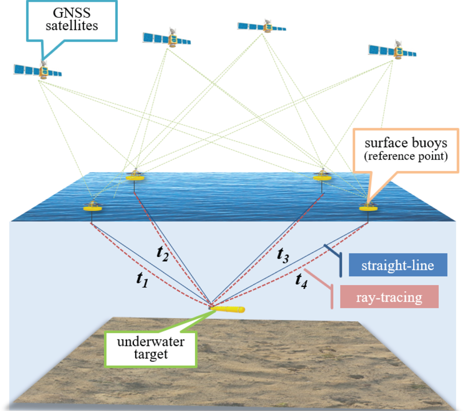
Figure 1. Diagram of a typical GNSS-acoustic intelligent buoys system (GIB).
2.1. Positioning principle of GIB system
The coordinates of reference points  $(x_i,y_i,z_i{\rm ) (}i = 1{\rm ,}\;2{\rm ,}\; \ldots {\rm ,}\;n)$ can be provided by the GNSS receivers, where i stands for the number of reference points. The system measures the travel time of acoustic signals t i from the reference points to the target. Assuming that the sound speed c is constant, the distances between the reference points and the target ρi are defined by
  $\rho_{i}={\textit{ct}}_{i}$. However, the acoustic path in the constant gradient sound speed layer is a circular arc (Kammerer, Reference Kammerer2000), so the variation of c in the vertical direction will cause refraction artefacts, which can lead to a large positioning deviation.
The non-difference observation equation can be given as
 $$\label{eq1} \rho _i =f_i +\delta d_i +\delta \textit{v}_i +\varepsilon _i$$
 where δ d i is the systematic error due to the time delay of the transducer,  $\delta {\textit{v}}_{i} $ is the systematic error due to spatial and temporal variations in sound speed, and
  $\varepsilon _{i} $ is the random ranging error. For target coordinates of (x t, y t, z t), f i represents the non-difference model, which can be described as follows:
 $$f_i = \sqrt {{(x_t-x_i)}^2 + {(y_t-y_i)}^2 + {(z_t-z_i)}^2} $$
The error equation and the normal equation can be expressed as
 $$\left\{ {\matrix{ {{\textbf V} = {\textbf AX}-{\textbf L}} \hfill \cr {{\textbf X} = {\left( {{\textbf A}^{\rm T}{\textbf A}} \right)}^{-1}{\textbf A}^{\rm T}{\textbf L}} \hfill \cr } } \right.$$
where
 $$\begin{align} \textbf{X}=[\begin{matrix} {\Delta x} & {\Delta y} & {\Delta z} \\ \end{matrix}]^{\rm T},\quad \textbf{A}=\left[\begin{matrix} {\dfrac{\partial f_1 }{\partial x}} & {\dfrac{\partial f_2 }{\partial x}} & \cdots & {\dfrac{\partial f_n }{\partial x}} \\\noalign{\vskip5pt} {\dfrac{\partial f_1 }{\partial y}} & {\dfrac{\partial f_2 }{\partial y}} & \cdots & {\dfrac{\partial f_n }{\partial y}} \\\noalign{\vskip5pt} {\dfrac{\partial f_1 }{\partial z}} & {\dfrac{\partial f_2 }{\partial z}} & \cdots & {\dfrac{\partial f_n }{\partial z}} \\ \end{matrix} \right]^{\rm T}, \quad \textbf{L}=\left[\begin{matrix} {f_1 -\rho_1 } \\ {f_2 -\rho_2 } \\ {\cdots} \\ {f_n -\rho_n } \end{matrix} \right]. \end{align}$$
This non-difference method is the most commonly used positioning calculation method, however, it ignores the impact of systematic errors.
2.2. Dilution of precision
As the available observation resources are often limited, the array shape of a GIB system is a crucial factor in the determination of its positioning accuracy (Sharp et al., Reference Sharp, Yu and Hedley2012). In this study, PDOP, HDOP and VDOP are used as evaluation standards to study the array network of a GIB system.
According to Equation (3), the matrix  $\textbf{A}^{\rm T}\textbf{A}$ is given as
 $${\textbf A}^{\rm T}{\textbf A} = \left[ {\matrix{ {\sum\limits_{i = 1}^n {h_{x_i}^2 } } & {\sum\limits_{i = 1}^n {h_{x_i}h_{y_i}} } & {\sum\limits_{i = 1}^n {h_{x_i}h_{z_i}} } \cr {\sum\limits_{i = 1}^n {h_{x_i}h_{y_i}} } & {\sum\limits_{i = 1}^n {h_{y_i}^2 } } & {\sum\limits_{i = 1}^n {h_{y_i}h_{z_i}} } \cr {\sum\limits_{i = 1}^n {h_{x_i}h_{z_i}} } & {\sum\limits_{i = 1}^n {h_{y_i}h_{z_i}} } & {\sum\limits_{i = 1}^n {h_{z_i}^2 } } \cr } } \right]$$
 where  $h_{x_i} = {\rm (}\partial f_i/\partial x{\rm ) ,}\;h_{y_i} = {\rm (}\partial f_i/\partial y{\rm ) ,}\;h_{z_i} = {\rm (}\partial f_i/\partial z{\rm )}$ are the cosines between the reference points and the target in three-dimensional directions. The PDOP of a non-difference method can be expressed as
 $${\rm PDOP} = \sqrt {tr{{\rm (}{\bf A}^{\rm T}{\bf A}{\rm )}}^{-1}} = \sqrt {tr\left( {{\rm diag}\left( {\displaystyle{1 \over {\lambda _1}},\displaystyle{1 \over {\lambda _2}},\displaystyle{1 \over {\lambda _3}}} \right)} \right)} $$
 where  $\lambda _i{\rm (}i = 1{\rm ,}\;2{\rm ,}\;3{\rm )}$ is a characteristic value of
  $\textbf{A}^{\rm T}\textbf{A}$. HDOP and VDOP are defined as
  ${\rm HDOP}=\sqrt {tr( {{\rm diag}( {1/\lambda_{1} {\rm ,} \; 1/\lambda_{2} } ) } ) } $ and
  ${\rm VDOP}=\sqrt {tr( {{\rm diag}( {1/\lambda_{3} } ) } ) } $; they satisfy the relationship
  ${\rm PDOP}^{2}={\rm HDOP}^{2}+{\rm VDOP}^{2}$. According to the definition of a matrix trace,
  $tr( \textbf{A}^{\rm T}\textbf{A} ) =\sum_{i=1}^{3} {\lambda _{i} =n} $ and
  ${\rm PDOP}\ge \sqrt 3 /n$ (Xue and Yang, Reference Xue and Yang2015). Optimal configurations with a certain number of reference points, such as triangles, tetragons, regular polygons and regular tetrahedrons, have been thoroughly studied and applied in network designs (Levanon, Reference Levanon2000).
3. SINGLE-DIFFERENCE DYNAMIC POSITIONING METHOD
The non-difference method, based on the least squares approach, is widely used in positioning calculations, however it cannot eliminate the influence of systematic errors. Xu et al. (Reference Xu, Ando and Tadokoro2005) proposed using the single-difference method for the positioning of static targets, however this method is difficult to apply to underwater dynamic positioning due to the lack of redundant measurements below a certain epoch. However, GIB systems can deploy several buoys on the water surface to provide sufficient redundant measurements for dynamic positioning. Therefore, in this study a single-difference dynamic positioning method is proposed to eliminate the influence of systematic errors by applying the difference operator to two measurements under the same epoch.
3.1. Principle of the single-difference method
Supposing that the coordinates of reference points are ( $x_{i}{\rm ,} \; y_{i}{\rm ,} \; z_{i}) ( i=1{\rm ,} \; 2{\rm ,} \; \ldots{\rm ,} \; n$), and that the coordinates of a difference reference point (x r, y r, z r) are added, all of the coordinates of the reference points and difference reference point can be provided by the GNSS receivers. The single-difference equation is given as
 $$\Delta \rho _{i,r} = F_{i,r} + \Delta \delta d_{i,r} + \Delta \delta v_{i,r} + \Delta \varepsilon _{i,r}$$
 where the difference in distance is  $\Delta \rho _{i{\rm ,} r} =\rho _{i} -\rho _{r} =( {t_{i} -t_{r} } ) \cdot c$, the single-difference model is
  $F_{i{\rm ,} r} =f_{i} -f_{r} $ and the difference in random error is
  $\Delta \varepsilon _{i{\rm ,} r} =\varepsilon _{i} -\varepsilon _{r} $. For the same transponder, the difference of time delays for systematic error is given by
  $\Delta \delta d_{i{\rm ,} r} =\delta d_{i} -\delta d_{r} \approx 0$. Across a small survey area, the difference in the systematic error of the sound speed is
  $\Delta \delta \textit{v}_{i{\rm ,} r} =\delta \textit{v}_{i} -\delta \textit{v}_{r} \approx 0$. Therefore, Equation (6) can be simplified as
  $\Delta \rho _{i{\rm ,} r} =F_{i{\rm ,} r} +\Delta \varepsilon _{i{\rm ,} r} $.
The normal equation is expressed as
 $${\bf X} = {\rm (}{\bf B}^{\rm T}{\bf B}{\rm )}^{-1}{\bf B}^{\rm T}{\bf L}$$
where
 $$\[ \textbf{X}=\left[\begin{matrix} {\Delta x} & {\Delta y} & {\Delta z} \\ \end{matrix}\right]^{\rm T},\quad \textbf{B}=\left[\begin{matrix} {\dfrac{\partial F_{1,r} }{\partial x}} & {\dfrac{\partial F_{2,r} }{\partial x}} & \cdots & {\dfrac{\partial F_{n,r} }{\partial x}} \\\noalign{\vskip5pt} {\dfrac{\partial F_{1,r} }{\partial y}} & {\dfrac{\partial F_{2,r} }{\partial y}} & \cdots & {\dfrac{\partial F_{n,r} }{\partial y}} \\\noalign{\vskip5pt} {\dfrac{\partial F_{1,r} }{\partial z}} & {\dfrac{\partial F_{2,r} }{\partial z}} & \cdots & {\dfrac{\partial F_{n,r} }{\partial z}} \\ \end{matrix} \right]^{\rm T},\quad \textbf{L}=\left[\begin{matrix} {F_{1,r} -\Delta \rho_{1,r} } \\\noalign{\vskip5pt} {F_{2,r} -\Delta \rho_{2,r} } \\\noalign{\vskip5pt} \cdots \\ {F_{n,r} -\Delta \rho_{n,r} } \end{matrix} \right]. \]$$
3.2. DOP of the single-difference method
For the shape of array network, optimal network structure based on DOP has been widely used. PDOP, HDOP and VDOP were used as the evaluation standards for the network analysis of the single-difference dynamic positioning method.
According to Equation (7),  $\textbf{B}^{\rm T} \textbf{B}$ is given as
 $$\label{eq8} \textbf{B}^{\rm T} \textbf{B}=\left[\begin{matrix} \displaystyle{\sum_{i=1}^n {H_{x_{i,r} }^2 } } & \displaystyle{\sum_{i=1}^n {H_{x_{i,r} } H_{y_{i,r} } } } & \displaystyle{\sum_{i=1}^n {H_{x_{i,r} } H_{z_{i,r} } } } \\\noalign{\vskip5pt} \displaystyle{\sum_{i=1}^n {H_{x_{i,r} } H_{y_{i,r} } } } & \displaystyle{\sum_{i=1}^n {H_{y_{i,r} }^2 } } & \displaystyle{\sum_{i=1}^n {H_{y_{i,r} } H_{z_{i,r} } } } \\\noalign{\vskip5pt} \displaystyle{\sum_{i=1}^n {H_{x_{i,r} } H_{z_{i,r} } } } & \displaystyle{\sum_{i=1}^n {H_{y_{i,r} } H_{z_{i,r} } } } & \displaystyle{\sum_{i=1}^n {H_{z_{i,r} }^2 } } \end{matrix}\right]$$
 where  $H_{x_{i{\rm ,} r} } =h_{x_{i} } -h_{x_{r} } $,
  $H_{y_{i{\rm ,} r} } =h_{y_{i} } -h_{y_{r} } $,
  $H_{z_{i{\rm ,} r} } =h_{z_{i} } -h_{z_{r} } $, and h x, h y, and h z are the cosines between the target and the reference points. The PDOP of a single-difference method is defined as
 $${\rm PDO}{\rm P}_{\rm d} = \sqrt {tr{{\rm (}{\bf B}^{\rm T}{\bf B}{\rm )}}^{-1}} = \sqrt {tr\left( {{\rm diag}\left( {\displaystyle{1 \over {\lambda _1}},\displaystyle{1 \over {\lambda _2}},\displaystyle{1 \over {\lambda _3}}} \right)} \right)} $$
 where  $\lambda _{i} ( {i=1{\rm ,} \; 2{\rm ,} \; 3} ) $ is the characteristic value of
  $\textbf{B}^{\rm T} \textbf{B}$. HDOPd and VDOPd are defined as
  ${\rm HDOP}_{\rm d} =\sqrt {tr( {{\rm diag}( {1/\lambda_{1} {\rm ,} \; 1/\lambda_{2} } ) } ) } $ and
  ${\rm VDOP}_{\rm d} =\sqrt {tr( {{\rm diag}( {1/\lambda_{3} } ) } ) } $; they satisfy the relationship
  ${\rm PDOP}_{\rm d} ^{2}={\rm HDOP}_{\rm d} ^{2}+{\rm VDOP}_{\rm d} ^{2}$. According to the definition of a matrix trace,
  $tr( {\textbf{B}^{\rm T} \textbf{B}} ) $ is given as
 $$tr{\rm (}{\bf B}^{\rm T}{\bf B}{\rm )} = \sum\limits_{i = 1}^3 {\lambda _i} = 2n-2\left( {\sum\limits_{i = 1}^n {h_{x_i}^2 h_{x_r}^2 } + \sum\limits_{i = 1}^n {h_{y_i}^2 h_{y_r}^2 } + \sum\limits_{i = 1}^n {h_{z_i}^2 h_{z_r}^2 } } \right)$$
 As shown in Figure 2(a), in the central region of a regular polygon network, the vertical angles between each reference point and the target are approximately equal, that is,  $\theta _{1} \approx \theta _{2} \approx \cdots \approx \theta _{n} \approx \theta _{r} $. The cosines between the target and the reference points are therefore also approximately equal, that is,
  $h_{x_{i} } \approx h_{x_{r} } {\rm ,} \; h_{y_{i} } \approx h_{y_{r} } {\rm ,} \; h_{z_{i} } \approx h_{z_{r} } $. In this case, according to Equation (10), the value of
  $tr( \textbf{B}^{\rm T} \textbf{B} ) $ will be zero or near zero. The value of PDOPd will be very large, however, which will result in an unfavourable solution. As shown in Figure 2(a), if the difference reference point is placed in the centre of the radiation network, the value of PDOP will be small across the central region of the survey area.

Figure 2. Schematic diagrams of (a) a regular polygon network and (b) a radiation network.
4. DOP SIMULATION OF SINGLE-DIFFERENCE METHOD
A simulation is required to verify the theoretical analysis. For the simulation in this study, the range of the survey area was assumed to be  $1{\rm ,} \; 500\, {\rm m} \times 1{\rm ,} \; 500\, {\rm m} \times 1{\rm ,} \; 500$ m, the spacing of DOP sampling points was assumed to be 1 m, and different array networks were adopted to calculate PDOP, HDOP and VDOP. Figure 3 shows a simulation in which the array has a regular quadrilateral-shaped network, and one of the reference points is selected as the difference reference point. In Figure 4, a radiation network has been adopted for the simulation, and an edge difference reference point is selected. In Figure 5, the centre reference point of a radiation network is selected as the difference reference point. In Figure 6, the non-difference method has been used with a radiation network. The statistical results are shown in Table 1.

Figure 3. (a) PDOP, (b) HDOP and (c) VDOP of a single-difference method with a quadrilateral network.

Figure 4. (a) PDOP, (b) HDOP and (c) VDOP of an edge-single-difference method with a radiation network.

Figure 5. (a) PDOP, (b) HDOP and (c) VDOP of a centre-single-difference method with a radiation network.

Figure 6. (a) PDOP, (b) HDOP and (c) VDOP of a non-difference method with a radiation network.
Table 1. PDOP statistics of the different array networks.

From Figure 3, it can be seen that 92·1% of the PDOP points have values that are >20, meaning that the calculation results of the single-difference method with a regular quadrilateral network would be greatly affected by systematic error. As shown in Figure 4, when the radiation network with an edge difference reference point is adopted, the DOP values decrease significantly, but 14·3% of PDOP points still have values >20. As shown in Figure 5, when the centre-difference reference point is used for the single-difference method, 98·4% of PDOP points have values <20. In Figure 6, when using the non-difference method, the DOP values are very small across the entire survey area.
According to the simulation results, the array shape of the single-difference method had a greater influence on the positioning calculation than that of the non-difference method. Adopting a radiation network with a centre-difference reference point effectively reduces the DOP value, and improves the stability of the single-difference positioning calculation result.
5. EXPERIMENT AND ANALYSIS
As shown in Figure 7, an experiment was carried out on the Songhua Lake in Jilin province, China to test the accuracy of the single-difference dynamic positioning method developed in this study. The Sonardyne Fusion 6G LBL system, which can be considered an inverse GIB system, was used in the experiment. The other instruments used include a Kongsberg Simrad EM 3000 multibeam system, Leica GNSS-1200 receivers, a Seatex MRU-05 motion reference unit and an AML sound speed profiler (Figure 8).

Figure 7. Location of the study area; inset shows the bathymetry of the lake bed.

Figure 8. (a) Transceiver, (b) transponder, (c) GNSS RTK, (d) MRU and (e) sound speed profiler.
5.1. Experimental results
Firstly, the underwater terrain was measured using the multibeam system, following which the transponder array was designed. The array network and target tracks are shown in Figure 9(a). Secondly, the transponder array was calibrated and the coordinates of the transponders (i.e. the reference points) were calculated. Thirdly, the submerged transceiver installed on the side of the ship was regarded as the target, and the transponder array and GNSS RTK (real-time kinematic) were used to locate the target. The SSP measured during the experiment is shown in Figure 9(b).

Figure 9. (a) Array network, target tracks and (b) sound speed profile.
The position of the transceiver provided by the GNSS RTK was regarded as standard. The non-difference method, the single-difference method with an edge reference point (Transponder 1002), and the single-difference method with centre reference point (Transponder 1008) were each used to calculate the position of the transceiver in turn, and the sound speed c = 1, 460 m/s was used to calculate the distance in each case. The curves of PDOP, HDOP and VDOP calculated using the different methods are shown in Figure 10; the curves of the positioning errors in each of the three-dimensional directions are shown in Figure 11. Standard deviation, σ, used as an indicator of the calculated results, can be calculated as follows:
 $$\sigma = \sqrt {\sum\limits_{i = 1}^n {{{\rm (}\hat{\beta }-\beta {\rm )}}^2/n} } $$
 where  $\hat{\beta }$ is the estimation and β is the standard value. Table 2 shows the standard deviation and DOP for each of the methods, where σp is the position standard deviation, σx, σy and σz are the three-dimensional components of position standard deviation.

Figure 10. (a) Curves showing changes in PDOP, (b) HDOP and (c) VDOP over time during the experiment.

Figure 11. Curves showing changes in the positioning errors in each of the three-dimensional directions over time during the experiment.
Table 2. Standard deviation and DOP ranges for the different methods used in this study.

5.2. Experimental analysis
The purpose of this experiment was to verify that the single-difference method can eliminate the influence of systematic error, and that a radiation network with a centre-difference reference point is superior to a regular polygon network when the single-difference method is used. The experimental results showed that the following.
1. The non-difference method based on least squares is currently the most widely used positioning calculation method. It can be seen that the positioning error of the non-difference method in the vertical direction was 1·859 m, meaning that systematic errors seriously affected the positioning accuracy in the vertical direction.
2. Using the single-difference method with an edge difference reference point improved positioning accuracy in the vertical direction. However, because the DOP values of this method were greater than for the non-difference method, the positioning accuracy in the horizontal direction was lower.
3. The single-difference method with a centre-difference reference point effectively improved positioning accuracy in the vertical direction. In addition, as all the PDOP values were <5·5, positioning accuracy in the horizontal direction did not decrease compared with the non-difference method.
In summary, the experimental results verified that the single-difference method with a radiation network can eliminate the influence of systematic errors. This finding has positive significance for improving the accuracy of underwater positioning with the GIB system.
6. CONCLUSION
Difference positioning methods have been widely used in the elimination of systematic errors. However, due to the lack of redundant measurements under a certain epoch, their application in underwater positioning is problematic. As GIB systems can provide sufficient redundant measurements, a single-difference dynamic positioning method based on a GIB system was proposed in this study. To study the influence of array shape on the underwater positioning accuracy, PDOP, HDOP and VDOP were used as evaluation standards for array network analysis. The simulation results showed that when the single-difference method was used for positioning calculations, the radiation network performed better than the regular polygon network. Using the LBL system, which can be seen as an inverse GIB system, in an experiment carried out on Songhua Lake, revealed that using the single-difference method with a centre-difference reference point can effectively eliminate systematic error, and improve vertical positioning accuracy from a metre- to a decimetre scale.
ACKNOWLEDGEMENTS
This work was supported by National Key R&D Programme of China (Grant Nos. 2016YFB0501700 and 2016YFB0501705), the Shandong Provincial Key R&D Programme (Grant No. 2018GHY115002) and Special Fund for Basic Scientific Research of Central Public Research Institutes (Grant No. TKS190302).


