I. INTRODUCTION
Microfocused synchrotron X-ray beams are a powerful tool for characterization and imaging of a range of materials at the microscale. The three main techniques for elemental, chemical, or structural analysis are X-ray fluorescence (XRF), X-ray absorption spectroscopy (XAS), and X-ray diffraction (XRD). The first two methods probe local electronic structure and can provide spatially-resolved elemental distributions and chemical state information. XRD is sensitive to long-range order and probes crystalline properties such as crystal phase, orientation, and strain (Abbey, Reference Abbey2013). Synchrotron XRD can provide information, which can be combined or correlated with XRF and XAS measurements, by measuring the sample crystallinity, impurities in the crystal lattice, or crystal structure itself (Chantler et al., Reference Chantler, Rae, Islam, Best, Yeo, Smale and Wang2012).
Absorption and diffraction experiments are typically carried out on separate specialized beamlines and are often used in series to provide complimentary information. XAS offers unique information to track short-range changes in the local electronic structure, but can be insensitive to changes in material phase or the presence of impurities (Filipponi et al., Reference Filipponi, Di Cicco, De Panfilis, Trapananti, Itie, Borowski and Ansell2001). However, post-experiment chemical analysis is often insufficient to identify these potential problems because certain types of contamination are reversible (e.g. with change in temperature). XRF can provide a solution to this, where detection of elemental concentrations as low as 10 ppm is now routine for practical scan times (Ryan et al., Reference Ryan, Siddons, Kirkham, Li, de Jonge, Paterson and De Geronimo2013; Fisher et al., Reference Fisher, Fougerouse, Cleverley, Ryan, Micklethwaite, Halfpenny and Spiers2015). In the case of crystalline materials, impurities can potentially be identified directly (if crystalline) or through small changes in the parent lattice as measured by XRD.
This paper presents a feasibility study of using the Maia detector array (Kirkham et al., Reference Kirkham, Dunn, Kuczewski, Siddons, Dodanwela, Moorhead and Pfeffer2010; Ryan et al., Reference Ryan, Siddons, Kirkham, Li, de Jonge, Paterson and Boesenberg2014), an advanced XRF detector system, for simultaneous XAS, XRD, and topological mapping. The Maia detector is a 20×20 array of silicon diode detectors with the central 4×4 replaced with a Mo collimating tube, which allows the incident X-ray beam to pass freely through the detector and on to the sample which is located downstream. In comparison with most other existing XRF detectors, the Maia possesses a relatively large solid angle and large number of energy-dispersive detector elements, which permits more XRF and XRD signal to be collected. Although the SLCam (Ordavo et al., Reference Ordavo, Ihle, Arkadiev, Scharf, Soltau, Bjeoumikhov and Hartmann2011; Scharf et al., Reference Scharf, Ihle, Ordavo, Arkadiev, Bjeoumikhov, Bjeoumikhova and Kuhbacher2011) , a pnCCD energy-dispersive area detector contains many more pixels of finer size, the low count rates it requires to accurately determine the photon energy results in a different trade-off between sensitivity and detector pixel resolution. The SLCam must also be used in either reflection (e.g. 90° to incident beam) or transmission mode, which present other challenges, but has proven successful for full field fluorescence mode X-ray absorption near edge structure (XANES) imaging (Tack et al., Reference Tack, Garrevoet, Bauters, Vekemans, Laforce, Van Ranst and Vincze2014). The aim in the present study is to use the Maia detector for mapping the X-ray absorption fine structure (XAFS) and the local crystallographic structure simultaneously. The most significant benefit is that the same detector and X-ray probe may be used for all measurements, meaning that no alignment or correlation between the different experiments is needed.
Instead of using multiple detectors in different positions, complete spectral information is collected over the full energy range of both the incident energy and fluorescence spectra and over a large solid angle by the Maia detector. The full measured spectrum contains a combination of XRF and XRD signal, providing elemental and crystallographic information. By scanning the incident X-ray energy over an appropriate range, the XAFS can be measured. The potential of the Maia detector for simultaneous XAFS and XRD was tested in a proof-of-principal experiment carried out on a polycrystalline dog-bone Ni foil specimen. The incident X-ray energy was scanned over the Ni K-edge while collecting XRF and XRD spectra in the Maia detector. The surface topography was determined using surface-dependent changes in self-absorption of the XRF signal, the XAFS of the foil was mapped, and grain substructure was examined by the XRD.
II. EXPERIMENTAL
A. Experimental setup
The experiment was performed at the X-ray fluorescence microscopy (XFM) beamline (Paterson et al., Reference Paterson, de Jonge, Howard, Lewis, McKinlay, Starritt and Siddons2011) at the Australian Synchrotron. The incident X-ray beam energy was scanned using the double crystal monochromator from 8.293 to 9.128 keV in 2 eV steps. The beam was focused to a spot size with full-width at half-maximum (FWHM) of 2×2 µm2 by Kirkpatrick–Baez (KB) mirrors on the surface of the 15 µm-thick Ni foil specimen. The foil had been completely recrystallized to decrease defect density and minimize residual elastic strain. The sample was located 10 mm downstream of the Maia detector as shown in Figure 1. At each incident X-ray energy the sample was scanned with respect to the incident X-ray beam over an area of 600×120 µm2 (horizontal × vertical), on-the-fly scanning was used in the horizontal axis and 2 µm steps were used in the vertical axis. The resulting spectra were collected in the upstream Maia detector. The Maia detector array has a collimating Mo mask placed on top to absorb any incident photons that would result in charge sharing between neighboring pixels; the mask defined the optimal sample-to-detector distance to be 10 mm. Owing to the Mo mask, the effective pixel area decrease slightly as a function of distance from the center of the detector; the relative sizes are depicted in Figure 1. The Maia detector operates in event mode whereby each photon detected by the Maia is tagged with the incident X-ray energy, sample position, detector pixel, and measured photon energy. Post-experiment data processing was used to separate the event data into fluorescence and diffraction components for analysis.

Figure 1. (Colour online) The experimental setup at the XFM beamline. The incident beam energy was selected by the double-crystal monochromators (DCM) before being focused by the KB mirrors and passing through the center of the Maia detector and onto the polycrystalline nickel foil specimen.
B. Data processing and analysis
Processing of the raw spectra for the XRF and XAFS analysis was carried out using the dynamic analysis method in GeoPIXE (Ryan & Jamieson, Reference Ryan and Jamieson1993; Ryan et al., Reference Ryan, Etschmann, Vogt, Maser, Harland, Van Achterbergh and Legnini2005). The large solid angle subtended by the Maia detector is partly responsible for the high sensitivity to elemental concentration compared with other detectors, because more signal can be collected. Another benefit of large solid angle is the ability to monitor the spatial distribution of the XRF across the detector as the sample is scanned. The change in the intensity distribution can be related to small local changes in surface topography and hence changes in self-absorption. This principal has been demonstrated before using a single (Geil & Thorne, Reference Geil and Thorne2014) or dual (Smilgies et al., Reference Smilgies, Powers, Bilderback and Thorne2012) XRF detectors where changes in surface orientation of up to 45° were measured in one direction (the plane containing the incident beam and detected XRF). The Maia's 384 detectors permit the determination of the surface normal in three dimensions and hence variations in height across the sample.
The intensity of the XRF signal measured in each detector pixel, Ik at a single point on the sample, where the subscript k refers to the individual detector pixel, is
 $$I_k = I_0{\rm \Omega} _k\epsilon _k\; \mathop \int \limits_0^T e^{ - \mu _{\rm i}s_{\rm i}}\; e^{ - \mu _{\rm f}s_{{\rm f}k}}\; ds_{\rm i},\; \; $$
where I 0 is this incident X-ray flux, Ω k is the solid angle subtended by pixel k with efficiency, ε k and T is the sample thickness. The attenuation coefficients at the incident and fluorescence energies are μ i and μ f, respectively. The path length traveled through the sample by the incident beam is s i and the path length traveled by the XRF through the sample to reach the kth detector pixel is s fk as shown in Figure 2. As shown by Geil et al., the distance s fk can be written in terms of s i and a purely geometrical factor, c k .
Figure 2. Geometry for describing the spatial variations in XRF intensity due to self-absorption as described in the text. The beam is incident in the positive z-direction. Changes in the sample surface orientation lead to a change in self-absorption, which is seen in the detector plane as a change in the spatial XRF intensity.
Geometrically, the vector sum
 $s_{\rm i}{\hat {\bi z}} + s_{{\rm f}k}\; {\hat {\bi d}}_k$
(where
$s_{\rm i}{\hat {\bi z}} + s_{{\rm f}k}\; {\hat {\bi d}}_k$
(where
 ${\hat {\bi z}} = [0,0,1]$
) must lie on the sample surface plane, therefore
${\hat {\bi z}} = [0,0,1]$
) must lie on the sample surface plane, therefore
 $${\hat {\bi n}} \cdot (s_{\rm i}\; {\hat {\bi z}} + s_{{\rm f}k}{\hat {\bi d}}) = 0$$
where the term in brackets has a direction parallel to the local surface, hence
 $$s_{{\rm f}k} = - \displaystyle{{{\hat {\bi z}} \cdot {\hat {\bi n}}} \over {\matrix{ {{\hat {\bi d}} \cdot {\hat {\bi n}}} \cr \; \cr}}} \; s_{\rm i} = c_ks_{\rm i}.$$
Substituting this into Eq. (1) for s
fk
and evaluating the integral, the XRF intensity in each detector pixel can be written as a function of the sample surface normal (provided
 ${\hat {\bi n}} \cdot {\hat {\bi z}} \lt 0$
)
${\hat {\bi n}} \cdot {\hat {\bi z}} \lt 0$
)
 $$I_k \propto \displaystyle{{I_0{\rm \Omega} _k\epsilon _k} \over {\mu _{\rm i} + c_k\mu _{\rm f}}},$$
where c k is the geometric factor, described in Eqn. (3), containing the direction vectors to each detector element and the unknown surface normal. The surface normal was then found by fitting this distribution to the measured XRF intensity at each point on the sample.
Once the direction of the surface normal,
 ${\hat {\bi n}}$
, at each point on the sample has been found, a relief map of the sample can be generated by integrating the surface gradient to find the relative height across the sample. The integration of gradient maps to find a quantity of interest is a problem of wide scope to which there are many different solutions, Saracchini et al., (Reference Saracchini, Stolfi, Leitão, Atkinson and Smith2012) have compared many of these approaches. The aim is to recover the relative sample surface height Z(x, y) at each x and y point on the sample from measurements of its gradient. That is we want to recover Z(x, y) from measurements of F(x, y) and G(x, y) where
${\hat {\bi n}}$
, at each point on the sample has been found, a relief map of the sample can be generated by integrating the surface gradient to find the relative height across the sample. The integration of gradient maps to find a quantity of interest is a problem of wide scope to which there are many different solutions, Saracchini et al., (Reference Saracchini, Stolfi, Leitão, Atkinson and Smith2012) have compared many of these approaches. The aim is to recover the relative sample surface height Z(x, y) at each x and y point on the sample from measurements of its gradient. That is we want to recover Z(x, y) from measurements of F(x, y) and G(x, y) where
 $$F{\rm (}x,y{\rm )} = \displaystyle{{\partial Z} \over {\partial x}},\; \; \; \; G(x,y) = \displaystyle{{\partial Z} \over {\partial y}}.$$
An overdetermined linear system (factor of 2) using finite-difference operators and the surface gradients is formed as follows. With the finite difference matrix operators D x , D y , operating in the x and y-directions respectively and the measured gradients F i , G i , which represent the corresponding gradient in the ith pixel in the image, the linear system can be written
 $$\left[ {\matrix{ {D_x} \cr {D_y} \cr}} \right]\left[ {Z_i} \right] = \left[ {\matrix{ {F_i} \cr {G_i} \cr}} \right]$$
and solved for the unknown image height Z i written as a column vector.
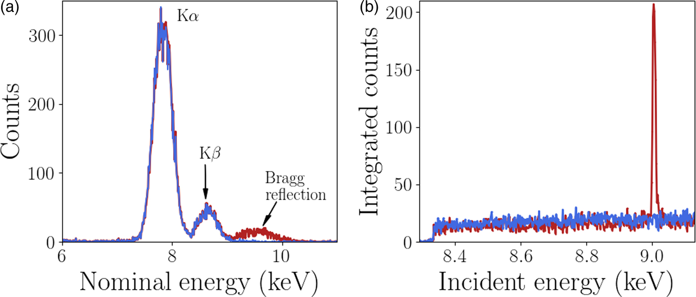
A custom GeoPIXE plugin was used to extract the diffraction data from each individual Maia detector element, this analysis is described here. The energy resolution of the monochromator (ΔE/E <1 × 10⁻⁴) is significantly higher than the energy resolution of each Maia detector element (ΔE/E ≈ 1 × 10⁻²). However, it has been shown by Robach et al., Reference Robach, Micha, Ulrich and Gergaud2011 that with increased measurement times and hence number of measured photons, the diffraction peak energy can be determined to an accuracy similar to the monochromator. In this case the monochromator was used to scan the energy for XANES imaging so the Maia energy resolution was not required for the diffraction peak analysis. The Maia energy resolution was used for the XRF analysis as the fluorescence peaks are typically brighter than the diffraction, an example of this is shown in Figure 3. To utilize the energy resolution of the monochromator the spectrum in the neighborhood of the incident beam energy in each Maia detector element was integrated over for each point in the scan (incident energy and sample position). The integrand contained both Ni fluorescence and diffraction signal when the incident energy was above the Ni K-edge absorption energy. The fluorescence signal has a smooth distribution over the detector whereas the diffraction is highly localized and easily detected. The resulting four-dimensional integrated intensity, a function of incident energy, sample position (horizontal and vertical) and detector pixel was input to a simple peak finding algorithm. The typical rocking curve width was of the order of 5 eV, peaks were easily located by the increase in signal in an individual Maia detector. A least-squares fit of a Gaussian function was applied to the peak to determine the height, peak position in energy, and width. An example of the spectra is shown in Figure 3. The energy resolution of the Maia detector and the monochromator are also compared, the diffraction peaks appear much wider in the Maia spectrum than in the monochromator spectrum. The events detected by the Maia were integrated over the range 7–12 keV to obtain the spectra shown in Figure 3(b), and used for the diffraction peak analysis. This broad energy range was to account for the peak broadening observed in the Maia spectra. Once the diffraction peaks were identified and fit parameters determined the grains and respective reflections were grouped for the crystallographic analysis. Changes in diffraction peak width and position can be related to local changes in the crystal lattice.

Figure 3. (Colour online) (a) The normalized spectra measured in two Maia detector elements. Bragg diffraction was detected with a peak at approximately 9.3 keV in one of the pixels. The peaks at approximately 7.8 and 8.6 keV are Ni fluorescence peaks as labeled with the emission type. The Ni XRF signal is much higher than the diffraction signal. (b) The XANES spectra with and without a Bragg reflection, the height of the peak was easily detected above the XRF signal.
III. RESULTS AND DISCUSSION
A. Absorption spectra
The XAFS and EXAFS spectra for the Ni foil are shown in Figure 4 and confirm that the sample was pure Ni to within the limits of detection. The XAFS signal for the pure Ni sample displayed very little change in chemical composition as a function of position on the sample as expected, but does provide some information about the grain surface structure. Figure 5 shows the relative height of the Ni K-edge, the grain boundaries are clearly distinguishable because of the decrease in fluorescence. The aim of this experiment was to test the feasibility of combined XAFS and XRD measurements with the Maia detector, to illustrate the diffraction analysis we focus on the diffraction signal measured from the single hexagonally shaped grain in the center of the scan region, as indicated in Figure 5.

Figure 4. Example of processed (a) XAFS and (b) EXAFS spectra from the Ni foil experiment.

Figure 5. (a) The relative height of the Ni surface over the scan region. The scale bar is 20 µm and the black box shows the location of the hexagonal grain used for the subsequent topographic and diffraction analysis. (b) Surface relief map of the grain used in the diffraction analysis. The color scale shows the surface height relative to the center of the hexagonally shaped grain determined by XRF self-absorption. (c) Scanning electron microscope image of the same region as shown in (b).
B. Surface relief determined from XRF self-absorption
The spatially varying direction of the surface normal was determined by fitting Eqn. (4) to the Ni XRF spectra measured in each Maia detector pixel. The efficiency of each Maia detector element, ε k , were determined from the spectra measured at multiple small areas on the sample that were deemed to be flat, i.e. distant from grain boundaries. A number of areas were used in the calibration. As an alternative this can also be done using a well-characterized sample to calibrate the detector efficiencies over a range of energies. The relative height at each pixel on the sample map was then determined by solving Eqn. (6) for the unknown height. The central region of the Ni foil was freely suspended and therefore had some curvature; a second order polynomial was fit to the surface height to account for this and subtracted to reveal the local surface topography. Figure 5(b) shows the surface height relative to the center of the hexagonal grain. The increased curvature and depth near the grain boundaries was confirmed by scanning electron microscopy measurements on the Ni foil.
C. Diffraction mapping
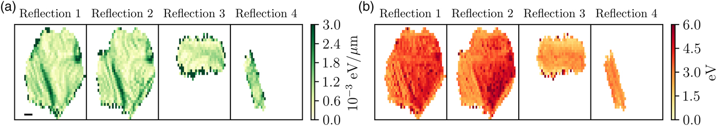
The Bragg diffraction peaks measured by the Maia detector in a single grain were analyzed next. Four reflections were detected from the hexagonal grain, the indexes could not be determined directly because of the angular resolution of the Maia detector, the direction between the incident and reflected beams could only be determined with certainty of 2°. Typically XRD experiments determine reflection directions with certainty of less than 0.1°. The locations and profiles of each reflection however still provide useful information about the crystal substructure without the need for indexing. The short range information provided by the XAFS measurements show the behavior at the sample surface, the diffraction information gives a more complex picture. In this case, the measured diffraction is sensitive to the full, through-thickness variation of the Ni foil (15 µm). In contrast to Electron backscatter diffraction (EBSD), a well-established method for mapping grain orientation in polycrystals, which is sensitive to grain orientation at the surface. Figure 6 shows the magnitude of the gradient of the peak energy and the full-width at half-maximum (FWHM). The magnitude of the gradient is proportional to local lattice rotation and the FWHM is sensitive to the size of the diffracting volume and variations in microstructure. The gradient and FWHM maps share features, which we can use to estimate the underlying crystal structure because the crystal orientation is unknown. There are two likely sources for the measured features. Both are because of the presence of twin boundaries, the diffraction peaks from the two twins is labeled reflection 3 and 4 in Figure 6. Nickel is well known to have low-angle twin boundaries (Abbey et al., Reference Abbey, Hofmann, Belnoue, Rack, Tucoulou, Hughes and Korsunsky2011), the change in FWHM in the reflections 1 and 2 around the grain boundary could therefore be attributed to the decreasing diffracting volume. Based on XRD and EBSD measurements on a similar region on the sample, the most likely explanation is that reflections 1 and 2 originate from a reciprocal lattice vector shared by the parent and twin grains, while reflections 3 and 4 originate from only the twin. The regions of increased gradient and FWHM are because of misorientation at the crystal-twin boundaries. Further description and an example of this phenomenon from a similar experiment are provided in the Supplemental Data section.

Figure 6. (Colour online) (a) The magnitude of the gradient of the peak energy. The scale bar in the bottom left corner is 10 µm. (b) The FWHM of the peaks for the four measured reflections from the hexagonal grain, the colorbar scale is in eV. Reflections 3 and 4 are from twinned crystals and appear to run parallel to the directions of the expected slip planes for FCC crystals.
A second possibility which would result in the structure in the diffraction maps is the presence of active slip planes. Electron back scatter diffraction measurements on a nearby region on the current sample, and in similarly prepared specimens (Hofmann et al., Reference Hofmann, Song, Jun, Abbey, Peel, Daniels and Korsunsky2010; Hofmann et al., Reference Hofmann, Abbey, Connor, Baimpas, Song, Keegan and Korsunsky2012a), show a preferential orientation where the [111]-direction is out of plane. This is one possible description for this hexagonal grain too as these features exhibit behavior consistent with the well-known slip directions in face-centered cubic (FCC) structure crystals (Jackson, Reference Jackson1991), where the slip planes are along the [110]-directions. The angles between two sets of slip planes in this regime is 60°. The same is observed in the hexagonal grain; corresponding to the directions of largest gradient and FWHM in reflections 1 and 2. The two smaller reflections, reflections 1 and 2, which are from the twinned areas, are a typical feature in highly annealed FCC metals, and run parallel to the slip planes. Further analysis or measurements are required to uniquely determine the underlying structure and source of the observed behavior. In either case the diffraction information has provided a more in depth look at the underlying structure, which was not apparent from the standard XAFS measurement.
IV. CONCLUSION
These results demonstrate the potential of the Maia detector for simultaneous XAFS and diffraction mapping. Although the sample has simple chemical composition feasibility has been demonstrated. In energy-scanned XAFS experiments involving crystalline samples and area detectors this information is measured but usually discarded. This work has shown the long-range structural information that can be extracted from such experiments. The diffraction revealed the presence of small lattice rotations and crystal twinning, which the XAFS measurement is insensitive to, but could influence surface chemistry. It could also be used to provide further context for elemental and chemical measurements. The potential to develop this for crystal orientation and strain studies also presents exciting prospects for studying deformation behavior (Korsunsky et al., Reference Korsunsky, Song, Hofmann, Abbey, Xie, Connolley and Drakopoulos2010) or the relationship between grains and grain boundaries (Hofmann et al., Reference Hofmann, Song, Dolbnya, Abbey and Korsunsky2009; Hofmann et al., Reference Hofmann, Song, Abbey, Jun and Korsunsky2012b), lattice dislocations, phase changes and chemical composition (Cahn et al., Reference Cahn, Pan and Balluffi1979; Guo et al., Reference Guo, Collins, Tarleton, Hofmann, Tischler, Liu, Xu, Wilkinson and Britton2015). Extending this to samples with more complicated elemental, chemical or crystallographic composition will require more in depth data analysis. This highlights the benefits of combining XRF, XANES, and XRD into a single technique to simultaneously obtain short range information about local atomic/molecular structure and long-range crystallographic information providing a more complete technique for materials analysis.
SUPPLEMENTARY MATERIAL
The supplementary material for this article can be found at https://doi.org/10.1017/S0885715617000768
ACKNOWLEDGEMENTS
This research was undertaken on the XFM beamline at the Australian Synchrotron, Victoria, Australia. The authors would like to thank AINSE Ltd for providing financial assistance (Award – PGRA no. 11749) to support this work and acknowledge the support of the Australian Research Council (ARC) Centre of Excellence for Advanced Molecular Imaging. FH acknowledges funding from Leverhulme Trust Research Project Grant RPG-2016-190. The authors would like to gratefully acknowledge Ondrej Muránskry (Australian Nuclear Science and Technology Organisation) for performing the electron microscopy included in this work.