2.1 The swirling jet facility

The investigation is carried out in a water facility. A schematic view of the experimental set-up, including the tomographic PIV set-up, is shown in figure 1. The swirling jet facility used in this study resembles a typical bluff-body combustor geometry (figure 1a). The swirl generator was designed by the International Flame Research Foundation (Dugué & Weber Reference Dugué and Weber1992). The fluid is supplied by a pump and subsequently divided into six equal parts before entering the swirl generator through six evenly distributed radial inlets. The arrows in the figure indicate the flow direction. The flow passes a moveable block swirler which consists of 12 adjustable guide vanes that allow the amount of swirl to be changed. After flowing through an annular channel with an inner diameter $D_{i}=18$  mm and an outer diameter $D_{o}=27$  mm, the jet issues into an octagonal water-filled tank which has a cross-sectional size of 600 mm (${\approx}22D_{o}$) and a height of 800 mm (${\approx}30D_{o}$). The height of the annular nozzle inside the octagonal bottom floor is $H=20$  mm. The tank is made of poly(methyl methacrylate) (acrylic glass) to ensure full optical access for illumination and tomographic imaging and the dimensions are large enough to resemble the conditions of a free jet. The symmetry axis of the jet is aligned with the $y$ axis in the measurement coordinate system with the origin located in the centre and at the end of the inner tube. The velocity components in the $x$, $y$ and $z$ directions are labelled as $u$, $v$ and $w$, respectively. The working fluid is water with a density of $998.1~\text{kg}~\text{m}^{-3}$ and kinematic viscosity of $0.9915~\text{mm}^{2}~\text{s}^{-1}$. The flow rate is regulated by a frequency-controlled submersible pump and the flow rate is fixed at $18~\text{l}~\text{min}^{-1}$. This results in a Reynolds number of 8500 based on the hydraulic diameter of the annular jet ($D_{h}=9$  mm) and mean outlet axial velocity $v_{0}=0.94~\text{m}~\text{s}^{-1}$. The integrated flow rate based on the measured axial velocity profile at the nozzle outlet is within 3 % of the direct measurement by a rotameter. In this study, the amount of swirl is characterized by the swirl number $S$, which is defined as the ratio of the flux of tangential and axial momentum times outer radius:

(2.1)$$\begin{eqnarray}S=\frac{\displaystyle \int _{0}^{2\unicode[STIX]{x03C0}}\int _{D_{o}/2}^{D_{i}/2}\unicode[STIX]{x1D70C}\overline{v}\overline{v_{\unicode[STIX]{x1D703}}}r^{2}\,\text{d}r\,\text{d}\unicode[STIX]{x1D703}}{\displaystyle \frac{D_{o}}{2}\int _{0}^{2\unicode[STIX]{x03C0}}\int _{D_{i}/2}^{D_{o}/2}\unicode[STIX]{x1D70C}\overline{v}^{2}r\,\text{d}r\,\text{d}\unicode[STIX]{x1D703}},\end{eqnarray}$$

where the azimuthal velocity component $v_{\unicode[STIX]{x1D703}}$ is calculated based on averaging of the profiles at the nozzle exit in the azimuthal direction and the overbar denotes time-averaged quantities. In this study, the swirl number is kept constant at $S=0.36$.

Figure 1. Schematic view of the experimental set-up. (a) Detail of the nozzle geometry and the swirl generator used. (b) General view of the tomographic PIV set-up.

2.2 Data acquisition

The flow field is measured using time-resolved tomographic PIV. A schematic view of the measurement system is shown in figure 1(b). Neutrally buoyant polyamide spherical particles of $56~\unicode[STIX]{x03BC}\text{m}$ mean diameter were employed as tracer particles at a concentration of around 0.65 particles $\text{mm}^{-3}$. The flow was illuminated by a double-pulse Nd:YLF laser (Quantronix Darwin Duo, $2\times 25~\text{mJ}~\text{pulse}^{-1}$ at 1 kHz) with a wavelength of 527 nm. The light scattered by the particles was recorded by a tomographic system composed of four HighSpeedStar 6 CMOS cameras ($1024\times 1024$ pixels, $5400~\text{frames}~\text{s}^{-1}$, pixel pitch of $20~\unicode[STIX]{x03BC}\text{m}$). Each camera was equipped with a Nikon 105 mm focal objective with a numerical aperture $f=32$ to allow focused imaging of the illuminated particles. The cameras were linearly arranged in a horizontal plane with a viewing angle of $90^{\circ }$, where the two outer cameras were positioned/oriented along the $x$ and $z$ directions, respectively. The laser beam is transformed by the use of optics into a cylindrical volume with a diameter of $1.2D_{o}$ and the height of the measurement domain is $1.8D_{o}$, resulting in a digital resolution of $21.6~\text{pixels}~\text{mm}^{-1}$. The choice of a cylindrical measurement volume eliminated the need for a lens-tilt mechanism to comply with the Scheimpflug condition. Moreover, the use of a cylindrical volume yields a more favourable condition for accurate volumetric reconstruction because the particle image density does not change with the viewing angle along the azimuth and decreases when moving towards the periphery of the jet. The average particle image density is approximately 0.045 particles per pixel. The images were captured in a single-frame mode at a recording frequency of 2.5 kHz (which is about two orders of magnitude larger than the frequencies of the coherent flow structures studied) to enable the visualization of the time-series phenomena. A total of $N=5000$ samples are taken to obtain a sufficient amount of data for the decomposition analysis. This corresponds to a total acquisition time of 2 s, which is more than 50 times the precession period.

Image preprocessing, volume calibration, self-calibration, reconstruction and three-dimensional cross-correlation-based interrogation were performed using LaVision DaVis 8.1.6. A three-dimensional calibration target was scanned through the measurement volume in order to obtain the mapping function between the camera and the laboratory coordinate systems. The initial calibration was then refined by using the volume self-calibration technique (Wieneke Reference Wieneke2008), yielding a misalignment of less than 0.05 pixels. The raw images were preprocessed with background intensity removal and particle intensity normalization. The reconstruction of the tomograms was performed by use of MLOS initialization (Atkinson & Soria Reference Atkinson and Soria2009) and 10 CSMART iterations with Gaussian smoothing after each iteration. The particle images were then interrogated using windows of final size $48\times 48\times 48$ voxels with an overlap factor of 75 %, resulting in a vector spacing of 0.56 mm in each measurement direction. The dimensions of the measurement volume are 72 points in the $x$ and $z$ directions and 89 points in the $y$ direction. The measurement error of the instantaneous velocities is $0.04v_{o}$ and the error on the time-averaged velocities is $0.005v_{o}$. The reader is referred to Percin, Vanierschot & van Oudheusden (Reference Percin, Vanierschot and van Oudheusden2017) for a more detailed discussion regarding the quality of the data and an error analysis.

2.3 Large-scale flow structure extraction

Tomographic PIV measurements provide a vast amount of measurement data. The challenge to analyse these data is to separate turbulent or apparently stochastic features from other coherent motions in the flow field. Usually, these coherent motions have much longer time and much larger length scales compared to stochastic motions of fine-scale turbulence. As such, they can be overlooked in data analysis as they are often ‘masked’ by the latter ones. Several methods exist for the extraction of large-scale flow structures from turbulent flow fields. The most widely used ones are classical Fourier decomposition, proper orthogonal decomposition (POD) or its variants (Lumley Reference Lumley1970; Sirovich Reference Sirovich1987; Boreé Reference Boreé2003), dynamic mode decomposition (Rowley et al. Reference Rowley, Mezić, Bagheri, Schlatter and Henningson2009; Schmid Reference Schmid2010; Williams, Kevrekidis & Rowley Reference Williams, Kevrekidis and Rowley2015) and very recently spectral proper orthogonal decomposition (SPOD) (Sieber, Paschereit & Oberleithner Reference Sieber, Paschereit and Oberleithner2016). In this study, we apply snapshot POD and SPOD. In both techniques, the velocity field is decomposed into a set of spatial modes $\unicode[STIX]{x1D731}_{i}(\boldsymbol{x})$ and temporal coefficients $a_{i}(t)$ as

(2.2)$$\begin{eqnarray}\boldsymbol{v}(\boldsymbol{x},t)=\bar{\boldsymbol{v}}(\boldsymbol{x})+\boldsymbol{v}^{\dagger }(\boldsymbol{x})=\overline{\boldsymbol{v}}(\boldsymbol{x})+\mathop{\sum }_{i=1}^{N}a_{i}(t)\unicode[STIX]{x1D731}_{i}(\boldsymbol{x}),\end{eqnarray}$$

where $\boldsymbol{v}$ is a velocity vector with components $u$, $v$ and $w$. The overbar denotes time-averaged quantities and hence only the fluctuating velocity field is decomposed. For the $N$ snapshots in time obtained by tomographic PIV, the temporal coefficients $\boldsymbol{a}_{i}=[a_{i}(t_{1}),a_{i}(t_{2}),\ldots ,a_{i}(t_{N})]^{\text{T}}$ and mode energies $\unicode[STIX]{x1D706}_{i}$ can be obtained by solving the eigenvalue problem

(2.3)$$\begin{eqnarray}\unicode[STIX]{x1D64D}\boldsymbol{a}_{i}=\unicode[STIX]{x1D706}_{i}\boldsymbol{a}_{i};\quad \unicode[STIX]{x1D706}_{1}\geqslant \unicode[STIX]{x1D706}_{2}\geqslant \cdots \geqslant \unicode[STIX]{x1D706}_{n}\geqslant 0,\end{eqnarray}$$

where the elements of the correlation matrix $\unicode[STIX]{x1D64D}$ are given by

(2.4)$$\begin{eqnarray}R_{i,j}=\frac{1}{N}\left\langle \boldsymbol{v}^{\dagger }(\boldsymbol{x},t_{i}),\boldsymbol{v}^{\dagger }(\boldsymbol{x},t_{j})\right\rangle .\end{eqnarray}$$

As spatial inner product $\langle \,,\,\rangle$, the $L^{2}$ norm is usually taken. The spatial modes are obtained by the projection of the fluctuating velocity fields onto the temporal coefficients as

(2.5)$$\begin{eqnarray}\unicode[STIX]{x1D731}_{i}(\boldsymbol{x})=\frac{1}{N\unicode[STIX]{x1D706}_{i}}\mathop{\sum }_{j=1}^{N}a_{i}(t_{j})\boldsymbol{v}^{\dagger }(\boldsymbol{x},t_{j}).\end{eqnarray}$$

If periodic coherent structures exist in the flow field, the matrix $\unicode[STIX]{x1D64D}$ has a diagonal wave-like structure, also named diagonal similarity (Sieber et al. Reference Sieber, Paschereit and Oberleithner2016). In SPOD, this similarity is augmented by filtering the correlation matrix $\unicode[STIX]{x1D64D}$ along the diagonals using a simple low-pass filter. This introduces the correlation matrix $\unicode[STIX]{x1D64E}$, defined as

(2.6)$$\begin{eqnarray}S_{i,j}=\mathop{\sum }_{k=-N_{f}}^{N_{f}}g_{k}R_{i+k,j+k},\end{eqnarray}$$

with $\boldsymbol{g}$ a vector of length $2N_{f}+1$ with filter coefficients and $N_{f}$ the filter width. The correlation matrix $\unicode[STIX]{x1D64E}$ can then substitute $\unicode[STIX]{x1D64D}$ in (2.3) and the velocity field is decomposed using $\unicode[STIX]{x1D64E}$ instead of $\unicode[STIX]{x1D64D}$. A study by Sieber et al. (Reference Sieber, Paschereit and Oberleithner2016) of different test cases shows that optimal results are obtained if the filter size is one or two times the period of the periodic structure in the flow field.

An important aspect in the flow-field analysis and decomposition using POD/SPOD is the identification of linked modes. For instance, the dynamical behaviour of periodic coherent structures, such as the PVC, is described by a mode pair. A mode pair is defined as two modes in the decomposition that have the same spectral content and a constant phase difference of $\pm \unicode[STIX]{x03C0}/2$. As such, reconstructing the flow field with a mode pair describes the precession of a coherent structure in the flow. A linked mode pair $a_{i}(t)$ and $a_{j}(t)$ can be identified by looking at the harmonic correlation of the eigenvectors of the dynamic mode decomposition of the temporal coefficients. More detailed information on the identification of the pairs can be found in the work of Sieber et al. (Reference Sieber, Paschereit and Oberleithner2016).

2.4 Triple velocity decomposition

As the large-scale coherent vortical structures found in swirling flows precess around the central axis of the jet, a simple Reynolds decomposition of the flow field into a mean and fluctuating part is not appropriate. This decomposition makes no distinction between the contributions of precession and turbulence to the fluctuating part of the velocity. A more appropriate decomposition under this circumstance is the triple velocity decomposition as first proposed by Hussain & Reynolds (Reference Hussain and Reynolds1970). In this decomposition, the instantaneous velocity field at time instant $t_{i}$ is decomposed into three parts: a time-averaged (mean) flow field $\overline{\boldsymbol{v}}$, a quasi-periodic component $\widetilde{\boldsymbol{v}}$ induced by large-scale coherent structures and a quasi-stochastic turbulent component $\boldsymbol{v}^{\prime }$ according to

(2.7)$$\begin{eqnarray}\boldsymbol{v}(\boldsymbol{x},t_{i})=\overline{\boldsymbol{v}}(\boldsymbol{x})+\widetilde{\boldsymbol{v}}(\boldsymbol{x},t_{i})+\boldsymbol{v}^{\prime }(\boldsymbol{x},t_{i}).\end{eqnarray}$$

The large-scale coherent component $\widetilde{\boldsymbol{v}}$ can be found by reconstruction of the velocity with the relevant mode pairs of the (S)POD decomposition as

(2.8)$$\begin{eqnarray}\widetilde{\boldsymbol{v}}(\boldsymbol{x},t)=\mathop{\sum }_{k}(a_{i}^{k}(t)\unicode[STIX]{x1D731}_{i}^{k}(\boldsymbol{x})+a_{j}^{k}(t)\unicode[STIX]{x1D731}_{j}^{k}(\boldsymbol{x})),\end{eqnarray}$$

where a mode pair $k$ consists of (S)POD modes with indices $i$ and $j$. The second-order statistical moments $\overline{\widetilde{v}_{l}\widetilde{v}_{m}}$ can be calculated (taking into account the orthogonality of the temporal coefficients, i.e. $\overline{a_{i}a_{j}}=\unicode[STIX]{x1D706}_{i}\unicode[STIX]{x1D6FF}_{ij}$) as

(2.9)$$\begin{eqnarray}\overline{\widetilde{v}_{l}\widetilde{v}_{m}}=\mathop{\sum }_{k}(\unicode[STIX]{x1D706}_{i}^{k}\unicode[STIX]{x1D6F7}_{il}^{k}\unicode[STIX]{x1D6F7}_{im}^{k}+\unicode[STIX]{x1D706}_{j}^{k}\unicode[STIX]{x1D6F7}_{jl}^{k}\unicode[STIX]{x1D6F7}_{jm}^{k}),\end{eqnarray}$$

where $l$ and $m$ are components of the vector $\unicode[STIX]{x1D731}$.

2.5 Linear stability analysis

Global LSA is employed to model the coherent velocity fluctuations, which are then compared to the coherent velocity fluctuations determined by the SPOD approach. The method is based on an eigenmode analysis of the linear operator determining the evolution of perturbations on the mean flow field. The governing equations are derived from the incompressible Navier–Stokes equations and the incompressible continuity equation. Employing the triple decomposition ansatz (see § 2.4), equation (2.7) is substituted into both of these equations and both are time-averaged and phase-averaged. By subtracting the time-averaged set of equations from the phase-averaged set of equations, one arrives at the governing equations for the coherent velocity fluctuations (Reynolds & Hussain Reference Reynolds and Hussain1972):

(2.10)$$\begin{eqnarray}\displaystyle \frac{\unicode[STIX]{x2202}\widetilde{\boldsymbol{v}}}{\unicode[STIX]{x2202}t}+\widetilde{\boldsymbol{v}}\boldsymbol{\cdot }\unicode[STIX]{x1D735}\overline{\boldsymbol{v}}+\overline{\boldsymbol{v}}\boldsymbol{\cdot }\unicode[STIX]{x1D735}\widetilde{\boldsymbol{v}} & = & \displaystyle -\frac{\unicode[STIX]{x1D735}\widetilde{p}}{\unicode[STIX]{x1D70C}}+\unicode[STIX]{x1D735}\boldsymbol{\cdot }(\unicode[STIX]{x1D708}(\unicode[STIX]{x1D735}+\unicode[STIX]{x1D735}^{\top })\widetilde{\boldsymbol{v}})\nonumber\\ \displaystyle & & \displaystyle -\,\unicode[STIX]{x1D735}\boldsymbol{\cdot }(\unicode[STIX]{x1D749}_{R}+\underbrace{\unicode[STIX]{x1D749}_{N}}_{{\approx}0}),\end{eqnarray}$$

(2.11)$$\begin{eqnarray}\displaystyle \unicode[STIX]{x1D735}\boldsymbol{\cdot }\widetilde{\boldsymbol{v}}=0, & & \displaystyle\end{eqnarray}$$

where $\unicode[STIX]{x1D749}_{N}=\widetilde{\boldsymbol{u}}\widetilde{\boldsymbol{u}}-\overline{\widetilde{\boldsymbol{u}}\widetilde{\boldsymbol{u}}}$ describes the nonlinear interactions of the perturbation with its higher harmonics (Mantič-Lugo, Arratia & Gallaire Reference Mantič-Lugo, Arratia and Gallaire2015). This term has zero mean and can be interpreted as the fluctuation of the coherent Reynolds stresses due to nonlinear interaction with the higher harmonics. It is assumed that these interactions are weak and the nonlinear term is neglected in the following. Turton, Tuckerman & Barkley (Reference Turton, Tuckerman and Barkley2015) state that the neglect of the nonlinear term is justified if the interaction of the fundamental with the higher harmonics is weak. In other words, it is assumed that the nonlinear energy transfer between the fundamentals and higher harmonics is weak compared to the energy transfer between mean and coherent field contained in the remaining linear terms of (2.10).

The other term $\unicode[STIX]{x1D749}_{R}=\langle \boldsymbol{v}^{\prime }\boldsymbol{v}^{\prime }\rangle -\overline{\boldsymbol{v}^{\prime }\boldsymbol{v}^{\prime }}=\widetilde{\boldsymbol{v}^{\prime }\boldsymbol{v}^{\prime }}$ describes the fluctuation of the stochastic Reynolds stresses due to the passage of a coherent perturbation (Reynolds & Hussain Reference Reynolds and Hussain1972). This term must be modelled in order to close (2.10).

As mentioned earlier, in the context of swirling flows with a PVC, it is now well established to use the Boussinesq eddy viscosity model as a closure (Oberleithner et al. Reference Oberleithner, Stöhr, Seong, Arndt and Steinberg2015; Rukes et al. Reference Rukes, Paschereit and Oberleithner2016; Tammisola & Juniper Reference Tammisola and Juniper2016). This is done here as well. It is also common to assume that the coherent fluctuations of the turbulent kinetic energy are small enough to be negligible (Reynolds & Hussain Reference Reynolds and Hussain1972). With that assumption one arrives at

(2.12)$$\begin{eqnarray}\unicode[STIX]{x1D749}_{R}=\widetilde{\boldsymbol{v}^{\prime }\boldsymbol{v}^{\prime }}=-\unicode[STIX]{x1D708}_{t}(\unicode[STIX]{x1D735}+\unicode[STIX]{x1D735}^{\top })\widetilde{\boldsymbol{v}}.\end{eqnarray}$$

The unknown eddy viscosity is calculated from the measured velocity fields of the experiment. As the turbulence of the swirling jet is highly anisotropic, the approach in (2.12) yields six independent eddy viscosities. A reasonable compromise among the six eddy viscosities can be achieved by using a least-squares fit over all resolved stochastic Reynolds stresses (Ivanova, Noll & Aigner Reference Ivanova, Noll and Aigner2013):

(2.13)$$\begin{eqnarray}\unicode[STIX]{x1D708}_{t}=\frac{\langle -\overline{\boldsymbol{v}^{\prime }\boldsymbol{v}^{\prime }}+2/3\cdot k\unicode[STIX]{x1D644},\overline{\unicode[STIX]{x1D64E}}\rangle _{F}}{2\langle \overline{\unicode[STIX]{x1D64E}},\overline{\unicode[STIX]{x1D64E}}\rangle _{F}},\end{eqnarray}$$

where $\langle \cdot ,\cdot \rangle _{F}$ is the Frobenius inner product, $k$ is the turbulent kinetic energy, $\unicode[STIX]{x1D644}$ is the identity tensor and $\overline{\unicode[STIX]{x1D64E}}=1/2\boldsymbol{\cdot }(\unicode[STIX]{x1D735}+\unicode[STIX]{x1D735}^{\top })\overline{\boldsymbol{v}}$ is the mean strain rate tensor. The eddy viscosity is then simply added to the kinematic viscosity to form an effective viscosity $\unicode[STIX]{x1D708}_{\text{eff}}=\unicode[STIX]{x1D708}+\unicode[STIX]{x1D708}_{t}$. The effective viscosity then replaces the kinematic viscosity in (2.10).

The global LSA examines flows which are inhomogeneous in two or three spatial dimensions. These are typically named bi-global and tri-global LSA (Theofilis Reference Theofilis2011). For the present work, a bi-global analysis suffices due to the homogeneity of the mean flow along the azimuthal direction. Equations (2.10) and (2.11) are solved with a normal mode ansatz in cylindrical coordinates:

(2.14)$$\begin{eqnarray}\widetilde{\boldsymbol{q}}(\boldsymbol{x},t)=\hat{\boldsymbol{q}}(\boldsymbol{x},r)\text{e}^{\text{i}(m\unicode[STIX]{x1D703}-\unicode[STIX]{x1D706}t)}+\text{c.c.},\end{eqnarray}$$

where $\hat{\boldsymbol{q}}$ are the complex spatial amplitude functions of the velocities and the pressure, $m$ is the azimuthal wavenumber and $\unicode[STIX]{x1D706}$ is the complex frequency. Discretization and rearrangement lead to a linear generalized eigenvalue problem with $\unicode[STIX]{x1D706}$ as eigenvalue. Solving the eigenvalue problem provides the eigenmodes $\hat{\boldsymbol{q}}$, each accompanied by one complex eigenvalue $\unicode[STIX]{x1D706}$. The eigenvalue consists of a real part $\text{Re}(\unicode[STIX]{x1D706})=\unicode[STIX]{x1D714}$ that corresponds to the angular frequency of the mode and of an imaginary part $\text{Im}(\unicode[STIX]{x1D706})=\unicode[STIX]{x1D70E}$ corresponding to the temporal growth rate. In the eigenspectrum, an oscillator mode at the limit cycle, such as the PVC, is expected to be an eigenvalue isolated from any continuous eigenvalue branch and approximately marginally stable ($\unicode[STIX]{x1D70E}\approx 0$) since the instability neither grows nor decays (Barkley Reference Barkley2006). With that criterion and the known frequency from the experiment, the single-helix and the double-helix vortex breakdown mode can be identified.

To obtain the adjoint modes, denoted with $(\cdot )^{+}$, the direct eigenvalue problem is reformulated as an adjoint eigenvalue problem being derived from the continuous formulation of the adjoint equations of (2.10) and (2.11) (Luchini & Bottaro Reference Luchini and Bottaro2014). The adjoint mode can be interpreted as the receptivity of the direct mode with regard to a periodic forcing (Sipp et al. Reference Sipp, Marquet, Meliga and Barbagallo2010). Furthermore, the structural sensitivity of an eigenvalue to mean flow modifications can be estimated via the Cauchy–Schwarz inequality from the direct and adjoint modes. The structural sensitivity is then defined by (Giannetti & Luchini Reference Giannetti and Luchini2007)

(2.15)$$\begin{eqnarray}\unicode[STIX]{x1D6EC}=\Vert \widetilde{\boldsymbol{v}}\Vert \cdot \Vert \widetilde{\boldsymbol{v}}^{+}\Vert .\end{eqnarray}$$

The regions of high structural sensitivity are interpreted as the wavemaker of the global instability. This is because the overlap of high amplitudes in both the direct and adjoint modes indicates the locations where the feedback among the coherent fluctuations is the strongest (Giannetti & Luchini Reference Giannetti and Luchini2007).

Table 1. Boundary conditions of the global direct LSA.

The Fortran code MAFIA (Paredes Reference Paredes2014) is employed for the discretization of the linearized Navier–Stokes and continuity equations (2.10) and (2.11), and for solving the eigenvalue problem with the Arnoldi algorithm. A high-order finite-difference scheme with non-uniformly distributed Chebyshev nodes is used for discretization. A total number of 8500 nodes is employed for a converged solution. The boundary conditions are set according to table 1. At the inlet, homogeneous Dirichlet boundary conditions for velocity and pressure are imposed since coherent fluctuations are not advected from upstream of the domain. At the outlet, homogeneous Neumann boundary conditions for the velocity and pressure are set since the domain is truncated at positions with remaining non-zero perturbations. For all walls, homogeneous Dirichlet boundary conditions are imposed for the velocity due to the no-slip and no-penetration condition. For the pressure, no physical boundary conditions exist. However, a compatibility condition from the governing momentum equations can be derived (Theofilis, Duck & Owen Reference Theofilis, Duck and Owen2004). Substituting the homogeneous Dirichlet conditions from the velocity into the linearized Navier–Stokes equation for the coherent perturbation, knowing that the eddy viscosity is zero as per definition on the wall, taking the inner product with the unit normal vector $\boldsymbol{n}$ at the respective boundaries, and rearranging leads to

(2.16)$$\begin{eqnarray}\displaystyle \frac{\unicode[STIX]{x2202}p}{\unicode[STIX]{x2202}n}=\unicode[STIX]{x1D70C}\unicode[STIX]{x1D708}\frac{\unicode[STIX]{x2202}^{2}v_{n}}{\unicode[STIX]{x2202}n^{2}}. & & \displaystyle\end{eqnarray}$$

Assuming $\unicode[STIX]{x2202}^{2}v_{n}/\unicode[STIX]{x2202}n^{2}\approx 0$ provides homogeneous Neumann conditions for the pressure on the walls. For the adjoint LSA, the same boundary conditions are applied as for the direct modes except that the outlet conditions from table 1 are set to homogeneous Dirichlet conditions. In the case of a converged adjoint solution, the adjoint eigenvalue $\unicode[STIX]{x1D706}^{+}$ of the PVC is the complex conjugate of the direct eigenvalue $\unicode[STIX]{x1D706}$. By that, the adjoint eigenmode can be identified.

3.1 Mean flow fields

The time-averaged flow field is shown in figure 2, where radial profiles of $\overline{v}/v_{0}$ and $\overline{w}/v_{0}$ are depicted. The profiles of $\overline{v}/v_{0}$ are wake-like due to the presence of the CRZ since the centrebody acts as a bluff body to the flow. This CRZ is toroidal due to the presence of the strong swirling component near the nozzle outlet as similarly observed by Vanierschot & Van den Bulck (Reference Vanierschot and Van den Bulck2008) and Sheen et al. (Reference Sheen, Chen and Jeng1996). Further downstream, a second recirculation zone appears, which is the vortex breakdown bubble. This recirculation zone is very weak as the maximum downward velocity is only $0.02v_{0}\pm 0.005v_{o}$. The azimuthal velocity profiles close to the central axis resemble a solid-body rotation ($\overline{w}=\unicode[STIX]{x1D6FA}y$) for $x/D_{o}\approx 0.9$ with an angular rotational frequency of $\unicode[STIX]{x1D6FA}=185~\text{rad}~\text{s}^{-1}$ (figure 2b).

3.2 Coherent structure extraction

Figure 2. Time-averaged flow field. The grey lines in the background denote streamlines. (a) Radial profiles of $\overline{v}/v_{0}$. (b) Radial profiles of $\overline{w}/v_{0}$.

Figure 3. Energy contribution of mode pairs to the dynamics of the flow using POD and SPOD. The diameter and colour of the points are a measure for the harmonic correlation and the mode pairs are numbered with decreasing harmonic correlation strength. Mode pair identification through (a) POD and (b) SPOD.

Recently, clear evidence of a double-helical structure has been identified in the flow field of the same annular jet flow in both the velocity and pressure fields (Percin et al. Reference Percin, Vanierschot and van Oudheusden2017; Vanierschot et al. Reference Vanierschot, Percin and van Oudheusden2018). This double helix has the same features as the single-helical PVC found in numerous other round or annular swirling jets: its branches are winded in the counter-swirl direction and the helix itself precesses along the central axis in the swirl direction. Analysis of the velocity spectra at different locations in the flow field showed a dominant peak at 28.2 Hz, corresponding to a Strouhal number based on the hydraulic diameter and mean jet outlet velocity, $St=fD_{h}/v_{0}$, of 0.27. A POD analysis of the pressure field (Percin et al. Reference Percin, Vanierschot and van Oudheusden2017) allowed both single- and double-helical structures to be identified, with corresponding Strouhal numbers of 0.28 and 0.56. As the frequency of the double helix was double that of the single helix, the authors speculated the double helix to be a higher harmonic of the single helix, as also shown by Oberleithner et al. (Reference Oberleithner, Sieber, Nayeri, Paschereit, Petz, Hege, Noack and Wygnanski2011). Besides this peak, several other peaks have been observed, corresponding to motions of the wake behind the central body (Vanierschot & Van den Bulck Reference Vanierschot and Van den Bulck2008; Vanierschot et al. Reference Vanierschot, Van Dyck, Sas and Van den Bulck2014). Hence, the annular jet is not only a very complicated flow field due to the presence of two interacting shear layers and associated anisotropic structure of turbulence, but it also contains many coherent structures with different time and length scales. Moreover, the possible coexistence of single- and double-helical structures and their possible relation or interaction have not been resolved and require further analysis.

Figure 4. Power spectral density of the first four mode pairs in the POD. The solid line corresponds to the first mode of the pair and the dashed line to the second one. Power spectral density of (a) mode pair I (modes 1 and 2), (b) mode pair II (modes 3 and 4), (c) mode pair III (modes 5 and 6) and (d) mode pair IV (modes 9 and 10).

Figure 5. Power spectral density of the first four mode pairs in the SPOD. The solid line corresponds to the first mode of the pair and the dashed line to the second one. Power spectral density of (a) mode pair I (modes 6 and 7), (b) mode pair II (modes 1 and 2), (c) mode pair III (modes 3 and 4) and (d) mode pair IV (modes 20 and 21).

An analysis of the mode pairs in the POD and SPOD and their associated energy contribution is shown in figure 3. The four mode pairs with the highest harmonic correlation are labelled. Modes with a high harmonic correlation represent oscillating or precessing motions. In the POD in figure 3(a), these four modes also have the highest energy content and hence represent dominating large-scale structures in the flow field. However, considering the frequency spectra of the temporal coefficients of these four pairs (figure 4), not one single but several distinct peaks are present. For instance the peak found at $St=0.27$ in the studies of Percin et al. (Reference Percin, Vanierschot and van Oudheusden2017) and Vanierschot et al. (Reference Vanierschot, Percin and van Oudheusden2018) can be found in mode pairs II and III. This indicates that contributions from several different structures in the flow with their own dynamics are present in a single mode pair. In other words, POD spreads out the coherent structures across multiple modes. Moreover, the double-helical structure found in the flow by other studies can only be observed in mode pair IV (more specifically, modes 9 and 10 of the POD). The energy content (around 3.9 %) is too low for the POD to separate it from other dynamical structures and noise in the data.

The mode pairs obtained by SPOD are shown in figure 3(b). A filter width of four to eight times the period of the motion to be studied was found to be the optimum. Increasing the filter width corresponds to narrowing the bandpass filter width in the spectrum of the coefficients (Sieber et al. Reference Sieber, Paschereit and Oberleithner2016). If the filter size $N_{f}$ and hence the spectral attenuation width are too small, several other peaks can be found in the spectra (similar to that for the conventional POD) and if the filter width is too large, the spectrum evolves towards a discrete Fourier transformation, which cannot take into account jitter in the frequency and modulation of the amplitude and is more prone to measurement noise. The optimal filter width obtained here is larger than the one found by Sieber et al. (Reference Sieber, Paschereit and Oberleithner2016), indicating the strong dependence of $N_{f}$ on the flow topology. One could say that a good procedure would be to take the smallest value for which the frequency spectra of the time coefficients show no frequency content from other flow structures.

In figure 3(b), the four pairs with the highest harmonic correlation are identical to those of the POD. However, the individual order is different as is also the energy content. The power spectral density of the temporal coefficients of these pairs is shown in figure 5. Pairs II and III correspond to motions of the wake and bubble (Vanierschot & Van den Bulck Reference Vanierschot and Van den Bulck2008; Vanierschot et al. Reference Vanierschot, Van Dyck, Sas and Van den Bulck2014). As the structures in these pairs have a rather low-frequency content, the filter size is too small to enhance the diagonal similarity and several peaks are therefore still present in the spectrum. These structures were also found in the POD and will not be considered further to limit the scope of the study, which focuses on the helical instabilities in the jet. Besides those modes, two other mode pairs displaying distinct frequencies emerge: a dominant one at $St=0.273\pm 0.005$ with 3.9 % energy content and a second one at $St=0.536\pm 0.005$ with 2 % energy content. In the following, we go into more detail of the dynamics of mode pairs I and IV.

3.3 Mode pair I: a single-helical PVC

Mode pair I in the SPOD spectrum in figure 3(b) consists of modes 6 and 7 (according to energy ranking) in the SPOD. The temporal coefficients, scaled with the single mode energy, are shown in figure 6(a). From the figure it is clear that the phase shift between the two time coefficients is $\unicode[STIX]{x03C0}/2$ as the minima and maxima of one coefficient correspond to the zeros of the other one and vice versa. Also the circular shape of the Lissajous curves (phase portraits) in figure 6(b) confirms this. Frequency spectra of the temporal coefficients (figure 5a) show a clear peak at 28.5 Hz or $St=0.273$ with equal magnitude for both coefficients of the pair. Figure 6(a) reveals that the single helix is not always present in the flow. The amplitude evolves from zero towards the limit cycle and back in a seemingly random way. This evolution in amplitude suggests that the mode is a marginally stable one and it gets excited by turbulent fluctuations or due to stochastic changes of the mean flow field (slow drift modes). More generally, in dynamical system theory the observation of a stable mode due to random forcing is also referred to as coherence resonance. Since the single-helical structure is not always present in the flow, it has a relatively low time-averaged energy content, making it very hard to be detected by POD. The spatial structure of the mode pair is shown in figure 6(c) and is visualized using the $Q$-criterion (Jeong & Hussain Reference Jeong and Hussain1995). Each mode consists of a double-helical structure and the phase angle between the two modes is $\unicode[STIX]{x03C0}/2$. Recombining the investigated mode pair with the mean flow field (figure 6d) shows a single-helical structure which is wrapped up in the counter-swirl direction upstream of the vortex breakdown bubble (visualized by the downstream black isocontour surface of zero axial velocity in the figure).

Figure 6. Temporal and spatial characteristics of mode pair I (modes 6 and 7 in the SPOD). (a) Evolution of the temporal coefficients. Solid line: $a_{6}(t)$; dashed line: $a_{7}(t)$. (b) Phase portrait. (c) Spatial structure of modes 6 and 7. Isocontours of $Q=0.25~\text{s}^{-2}$. Blue: mode 6; red: mode 7. (d) Reconstructed velocity field with only mode pair I. The light blue lines are isovalues of $Q=0.04~\text{s}^{-2}$ and the black surfaces are isosurfaces of zero axial velocity.

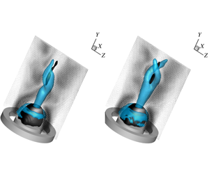
Figure 7. Temporal and spatial characteristics of mode pair IV (modes 20 and 21 in the SPOD). (a) Evolution of the temporal coefficients. Solid line: $a_{20}(t)$; dashed line: $a_{21}(t)$. (b) Phase portrait. (c) Spatial structure of modes 20 and 21. Isocontours of $Q=0.5~\text{s}^{-2}$. Blue: mode 20; red: mode 21. (d) Reconstructed velocity field with only mode pair IV. The light blue lines are isovalues of $Q=0.035~\text{s}^{-2}$ and the black surfaces are isosurfaces of zero axial velocity.

3.4 Mode pair IV: a double-helical PVC

Mode pair IV in the SPOD spectrum in figure 3(b) consists of modes 20 and 21 in the SPOD. The temporal coefficients are shown in figure 7(a). Similar to mode pair I, the phase shift between the time coefficients is $\unicode[STIX]{x03C0}/2$, again confirmed by the circles in the Lissajous curves (phase portraits) in figure 7(b). Frequency spectra of the coefficients in figure 5(d) show a clear peak at 56 Hz or $St=0.536$ which is equal in magnitude for both coefficients. This frequency is double the frequency of mode pair I within measurement accuracy. Together with the observation that the azimuthal wavenumber is also double, one might think that the double helix is the first harmonic of the single helix. However, figure 8 shows that mode pair IV is not a higher harmonic of mode pair I. If this were the case, the Lissajous curves in figure 8(a) should have a figure-of-eight shape. Nevertheless, plotting the phase portrait might be corrupted by intermittence and phase distortion of both modes and therefore a more detailed statistical analysis is given in figure 8(b,c). If the two modes were harmonics of each other, the plot of $\unicode[STIX]{x1D719}_{IV}$ versus $\unicode[STIX]{x1D719}_{I}$ should give an arrangement of the dots in three major diagonals, where $\unicode[STIX]{x1D719}_{I}=\arctan (a_{6}/a_{7})$ and $\unicode[STIX]{x1D719}_{IV}=\arctan (a_{20}/a_{21})$ are the phase angles of the mode pairs. The scattering of the data shows that this is clearly not the case. Also, if one were to plot the statistical histogram of the variable $2\unicode[STIX]{x1D719}_{I}-\unicode[STIX]{x1D719}_{IV}$, and the modes happen to be harmonics of each other, the fixed phase relation should give one clear peak in the histogram. Figure 8(c) shows that there is no statistical correlation, and hence it can be concluded that the modes are not harmonics of each other.

Figure 8. Analysis of the correlation between the phase angle of mode pair I and that of mode pair IV. (a) First temporal coefficient of mode pair IV versus mode pair I. (b) Phase angle of mode pair I versus mode pair IV. (c) Histogram of the phase difference of mode pair I and mode pair IV.

Figure 7(a) shows that mode pair IV is not always present in the flow, similar to the observations made for mode pair I. Comparison of figures 6(a) and 7(a) shows that there is no clear correlation between the appearance of the single and double helix in the flow field as both modes can coexist for some time intervals, while for other intervals only one of the two is present. Also, mode pair IV is more dynamic compared to mode pair I as the amplitude grows/decays more often. The spatial structure of mode pair IV is shown in figure 7(c). This indicates two different regions where the vortical structures are oriented differently. In the breakdown region the mode has a helical structure, similar to mode pair I, but in the wake region the vortical structures are oriented along the streamwise direction. The orientation of the vortices indicates different orientations of the mean strain rates that produce the vorticity. In the breakdown region, the superposition of axial and azimuthal velocities gives rise to helical vortical structures. In contrast, there is little axial velocity in the wake region behind the bluff body of the jet, which leads to a streamwise orientation of the vorticity. The mode shape indicates a linked dynamic in the two regions, which is in contrast to the single-helical structure. Recombining the flow field (figure 7d) reveals a double-helical structure which is wrapped up in the counter-swirl direction upstream of the vortex breakdown bubble (visualized by the downstream black isocontour surface of zero axial velocity in the figure). Once reconstructed in combination with the mean flow field, both structures precess at an angular frequency $\unicode[STIX]{x1D714}=2\unicode[STIX]{x03C0}f/m$, where $m$ is the azimuthal wavenumber and $f$ is the frequency corresponding to the peak in the power spectral density of the corresponding temporal mode coefficients. This results in a phase rotation rate of $\unicode[STIX]{x1D714}=180~\text{rad}~\text{s}^{-1}$ for both structures as the frequency peak of the double helix is more or less double that of the single helix and the azimuthal wavenumber is also double. This value is very close to the bulk rotation rate of the jet at the axial location where the cores break up, $\unicode[STIX]{x1D714}=185~\text{rad}~\text{s}^{-1}$, defined as the slope at the axis of the radial profiles of rotational velocity just upstream of the vortex breakdown bubble (figure 2b).

Figure 9. Coherent contribution to the second-order statistics of the single-helical (a–c) and double-helical (d–f) precession: (a) $\overline{\widetilde{u}\widetilde{u}}/v_{0}^{2}\times 100$; (b) $\overline{\widetilde{v}\widetilde{v}}/v_{0}^{2}\times 100$; (c) $\overline{\widetilde{w}\widetilde{w}}/v_{0}^{2}\times 100$; (d) $\overline{\widetilde{u}\widetilde{u}}/v_{0}^{2}\times 100$; (e) $\overline{\widetilde{v}\widetilde{v}}/v_{0}^{2}\times 100$; (f) $\overline{\widetilde{w}\widetilde{w}}/v_{0}^{2}\times 100$.

The dynamics of the two large-scale structures in the flow introduces extra mixing in the flow field. To quantify this mixing, figure 9 shows the contribution of both precessions to the second-order statistics (called the coherent stresses) of the flow. The single helix has the highest coherent stresses near the region where the central vortex core breaks up in a single helix. Slightly upstream of the bubble, the horizontal velocity components ($u$ and $w$) have the highest fluctuations, while for the axial velocity $v$ the fluctuations are highest in the shear layer between the vortex breakdown bubble and the jet. The double helix shows a different behaviour. Both $u$ and $w$ show large values in a region immediately downstream of the CRZ and in the shear layer between the vortex breakdown bubble and the jet. Comparison with the statistical data of Percin et al. (Reference Percin, Vanierschot and van Oudheusden2017) shows that despite the low energy content of the two precession motions (around 4 % and 2 %, respectively), the impact on the second-order statistics in the near-bubble region is significant with contributions of around 16 % for $\overline{\widetilde{u}\widetilde{u}}$ and $\overline{\widetilde{v}\widetilde{v}}$ and of 30 % for $\overline{\widetilde{w}\widetilde{w}}$. Analogous to the production of turbulent kinetic energy caused by mean shear, the contribution of the coherent flow component to the production of the kinetic energy can be written as

(3.1)$$\begin{eqnarray}P=-\overline{\tilde{v}_{j}\tilde{v}_{i}}\frac{\unicode[STIX]{x2202}\overline{v}_{i}}{\unicode[STIX]{x2202}x_{j}},\end{eqnarray}$$

where the expression is written in Einstein notation. The production of coherent kinetic energy for the two helical modes is shown in figure 10. High values indicate regions where the coherent structures extract energy from the mean flow. It can be seen that both the single and double helices extract energy from the shear layer between the vortex breakdown bubble and the jet, albeit somewhat more downstream for the double helix, while the former extracts more energy. The double helix also extracts a smaller amount of energy from the mean flow at the end of the CRZ.

Figure 10. Kinetic energy production $P$ ($\text{m}^{2}~\text{s}^{-3}$) of (a) the single helix and (b) the double helix.

4.1 Frequency, growth rate and mode structure

The eigenvalues obtained by the global direct LSA are displayed in figure 11. The spectrum is entirely stable since the growth rate of every eigenvalue is below the stability limit with $\unicode[STIX]{x1D70E}<0$. The eigenvalues marked with filled symbols correspond to the selected modes of interest that represent the single- and double-helical modes in the best possible way within the constraints of the normal mode basis. Further elaborations on convergence and accuracy of the eigenspectrum are provided in appendices A and B. Considering the single-helical spectrum (azimuthal wavenumber $m=1$), the least stable eigenvalue represents the single-helical mode found in the experiment. Its frequency of $St=0.268$ is very similar to the experimentally measured frequency of $St=0.273$ with a relative error of less than 2 %. For the double-helical spectrum (azimuthal wavenumber $m=2$), the eigenvalue with a frequency of $St=0.464$ represents the double-helical mode found in the experiment. In this case, the error relative to the experimentally obtained Strouhal number is approximately 13 %. The larger mismatch can be attributed to the position of the wavemaker, related to regions of recirculation in conjunction with the strong mean flow gradients occurring in its vicinity. Since the predicted LSA frequency is quite sensitive with regard to changes of the swirl velocity in the wavemaker region, any measurement error of tomographic PIV has a significant impact. This is likely to be the cause for the frequency mismatch. This is further shown and discussed in appendix A.

Figure 11. Eigenvalue spectrum with non-dimensional growth rate $\unicode[STIX]{x1D70E}D_{h}/v_{0}$ over Strouhal number $St$ obtained by global direct LSA of the mean flow for azimuthal wavenumber $m=1$ and $2$. Filled symbols (●, ▪) denote the identified single-helical and double-helical modes, vertical solid lines denote the experimentally measured Strouhal numbers and the horizontal dashed line denotes the stability limit.

The growth rates being close to but below the stability limit ($\unicode[STIX]{x1D70E}\lesssim 0$) reflect the property of both global modes existing only due to continuous stochastic forcing. The small negative values of the growth rates indicate that the modes only decay very slowly over large periods of time (note that the time scale of decay is more than an order of magnitude larger than the time scale of oscillation). However, for short periods of time, the modes can still transiently grow when stochastic forcing is applied. For the single-helical mode ($m=1$), the growth rate is associated with an error due to domain truncation at the outlet boundary. A shift of the outlet boundary in the upstream direction of up to 30 % results in an increase of the negative growth rate (see appendix C). This is associated with the truncation of the region of high structural sensitivity (shown and discussed further below), meaning that a significant part of the wavemaker centred around $y/D_{o}\approx 1.3$ is excluded. Therefore, it can be expected that the correct growth rate of the single-helical mode is actually even closer to the stability limit. In the case of the double-helical mode ($m=2$), no sensitivity of the growth rate due to domain truncation is identified. This is attributed to the primary wavemaker being located far upstream at the end of the recirculation bubble, concentrated around $y/D_{o}\approx 0.4$.

Figure 12. Spatial structure of the identified PVC modes obtained by global direct LSA; isosurface of $Q$ criterion (arbitrary scale and arbitrary phase angle); blue, real part; red, imaginary part. Vector field shows the real part of the coherent fluctuations projected onto the plane $x=0$. (a) Single-helical mode ($m=1$). (b) Double-helical mode ($m=2$).

The spatial structure of both single- and double-helical modes, based on the $Q$ criterion, is shown in figure 12. Comparing the mode of $m=1$ extracted via SPOD (see figure 6) to the mode predicted by global LSA, it is evident that a good match exists in some parts, while in other parts a slight mismatch can be observed. The inclination angle of the isosurfaces representing the counter-winding vortices is associated with the axial wavelength and it can be seen that prediction and measurement match very well. The increasing radial spread in the downstream direction is related to the convective growth and the LSA correctly captures this property. Additionally, the location where the mode starts to initially grow is predicted accurately as well. For $m=2$ (compared to figure 7), there are also clear similarities, although there is some mismatch too. The initiation of the double-helical mode far upstream at the end of the recirculation bubble is correctly predicted including the large axial wavelengths, resulting in a very small inclination angle of the counter-winding vortices. Downstream of the bubble, the mode decays at first, before it is again amplified in the axial direction. This trend is reproduced by the LSA mode as well. In the second region of convective amplification, the axial wavelength is slightly underpredicted compared to the SPOD mode, leading to a steeper inclination angle of the counter-winding vortices. Furthermore, the convective growth is overpredicted, leading to a larger radial spread of the mode. The mismatch towards the outlet boundary is likely to have the same cause as the mismatch of the frequency, which is rooted in potential inaccuracies in the wavemaker region due to very strong mean flow gradients.

4.2 Structural sensitivity and wavemaker

Figure 13 shows the structural sensitivity of the two identified global modes. This is high where the receptivity, represented by the adjoint mode, and the forcing, represented by the direct mode, have their combined maximum. These regions of high structural sensitivity correspond to the wavemaker of the respective modes where the self-excitation mechanism acts. In both cases the wavemaker positions are associated with regions of mean recirculation, supporting a self-excited feedback loop due to reverse flow. The wavemaker of the single-helical mode is located in the centre of the vortex breakdown bubble around $y/D_{o}\approx 1.3$. This thin recirculation strip, associated with the single-helix wavemaker, is completely detached from the upstream large recirculation bubble located at the exit of the annulus. For the double-helical mode, two wavemakers exist. The first is located at the downstream end of the recirculation bubble around $y/D_{o}\approx 0.4$ and is responsible for the initial growth of the amplitude as observed in figure 12. The second wavemaker is bordered at the vortex breakdown bubble, close to the wavemaker of the single-helical mode. It is responsible for the re-initiation of growth towards the downstream end of the domain. The first, upstream-lying wavemaker is the primary wavemaker of the mode since the truncation of the second, downstream-lying wavemaker does not affect the frequency and the growth rate of the double-helical mode, as discussed above (also see appendix C). The clear spatial separation of the single-helical wavemaker and the primary double-helical wavemaker demonstrates the independence of the self-excitation mechanisms. The double helix is explicitly no higher harmonic of the single helix and both modes have completely different sources. Moreover, the close proximity of the single-helical wavemaker and the secondary double-helical wavemaker coincides with the competition of both modes as observed for the temporal coefficients in figures 6 and 7. Notably, the bulk production of coherent kinetic energy (see figure 10) for both modes is slightly spatially shifted with the single-helical and secondary double-helical wavemaker. The maximum of production is reached slightly upstream of these wavemakers. This reflects an essential feature of both global modes. Coherent fluctuations are produced and subsequently advected downstream where they are fed to their respective wavemakers, sustaining the loop of self-excitation. Surprisingly, however, this does not apply to the primary wavemaker of the double helix. There, the main production starts downstream of the wavemaker.

Figure 13. Structural sensitivity $\unicode[STIX]{x1D6EC}$ of the identified global modes obtained by global direct and adjoint LSA. Grey lines denote streamlines and thick blue lines denote contours of zero axial velocity indicating the recirculation zones. (a) Single-helical mode ($m=1$). (b) Double-helical mode ($m=2$).