Introduction
Laser-induced breakdown spectroscopy (LIBS) is an analytical technique (Zhang et al., Reference Zhang, Yueh and Singh1999) that uses a laser to generate plasma from the target samples. The method is focusing a high power laser on a small surface area of the target sample (Popov et al., Reference Popov, Labutin, Zaytsev, Seliverstova, Zorov, Kal'ko, Sidorina, Bugaev and Nikolaev2014; Choi et al., Reference Choi, Choi and Yoh2016; Shaheen et al., Reference Shaheen, Irfan, Khan, Islam, Islam and Ahmed2016), which then ablates the surface to generate the plasma. The emitted radiations from the plasma are collected and processed to attain the quantitative and qualitative data on the target sample elemental composition. LIBS has been employed in a vast number of applications such as forensics (Bridge et al., Reference Bridge, Powell, Steele and Sigman2007; Naes et al., Reference Naes, Umpierrez, Ryland, Barnett and Almirall2008; Rodriguez-Celis et al., Reference Rodriguez-Celis, Gornushkin, Heitmann, Almirall, Smith, Winefordner and Omenetto2008), pharmaceuticals (Asimellis et al., Reference Asimellis, Hamilton, Giannoudakos and Kompitsas2005), military and security (Harmon et al., Reference Harmon, DeLucia, McManus, McMillan, Jenkins, Walsh and Miziolek2006; Gottfried et al., Reference Gottfried, De Lucia, Munson and Miziolek2008), environmental analyses (Corsi et al., Reference Corsi, Palleschi, Salvetti and Tognoni2002; Lei et al., Reference Lei, Motto-Ros, Boueri, Ma, Zhang, Zheng, Zeng and Yu2009; Boueri et al., Reference Boueri, Motto-Ros, Lei, Zheng and Zeng2011), archeological analyses (Müller and Stege, Reference Müller and Stege2003; Carmona et al., Reference Carmona, Oujja, Rebollar, Römich and Castillejo2005; Giakoumaki et al., Reference Giakoumaki, Melessanaki and Anglos2007), and material processing (Awan et al., Reference Awan, Ahmed, Aslam, Qazi and Baig2013; Sun et al., Reference Sun, Zhong, Lu, Sun, Ma and Liu2015; Li et al., Reference Li, Tian, Ding, Yang, Liu, Wang and Han2018; Markiewicz-Keszycka et al., Reference Markiewicz-Keszycka, Casado-Gavalda, Cama-Moncunill, Cama-Moncunill, Dixit, Cullen and Sullivan2018). The LIBS technique has gained an unprecedented attention from scientist all over the world from plasma physics, chemical physics, and material sciences (Neogi and Thareja, Reference Neogi and Thareja1999), due to its ability for in situ analysis, little or no sample preparation, fast and remote detection, and multi-elemental diagnosis. This technique can also be utilized to analyze all forms of matter irrespective of its physical state from solids (Sturm et al., Reference Sturm, Peter and Noll2000), liquids (Michel et al., Reference Michel, Lawrence-Snyder, Angel and Chave2007), and gases (Cremers and Radziemski, Reference Cremers and Radziemski1983; Radziemski and Cremers, Reference Radziemski and Cremers1989; Lee et al., Reference Lee, Song and Sneddon1997; Sturm and Noll, Reference Sturm and Noll2003). LIBS offers more advantages over other spectroscopic techniques such as mass spectroscopy, the electrode spark, and the inductively coupled plasma (Amoruso et al., Reference Amoruso, Bruzzese, Spinelli and Velotta1999). One of the significant challenges of LIBS is its low sensitivity, in spite of the advantages of the LIBS technique. Over the past decades to improve the LIBS sensitivity, numerous papers on the enhancement of the signal sensitivity of the LIBS technique have been reported using either cavity or magnetic confinement (Popov et al., Reference Popov, Colao and Fantoni2009). Research has been published (Guo et al., Reference Guo, Hu, Zhang, He, Li, Zhou, Cai, Zeng and Lu2011) on the study of combined spatial and magnetic confinements using both permanent magnets and hemispherical cavity in the LIBS for Co and Cr metallic samples.
Guo et al. (Reference Guo, Hao, Shen, Xiong, He, Xie, Gao, Li, Zeng and Lu2013) have studied the accuracy of quantitative analysis improvement of low concentration elements of a laser-induced steel plasma confined in a cavity using an Nd:YAG laser in the air. They investigated several elements with low concentrations, such as vanadium (V), chromium (Cr), and manganese (Mn). A significant enhancement in the emission intensities of the elements such as V, Cr, and Mn was observed, with an enhancement factor of 4.2, 3.1, and 2.97, respectively. Their results predicted that the accuracy of quantitative analysis by spatial confinement was improved.
Shao et al. (Reference Shao, Wang, Guo, Chen and Jin2017) also employed a Q-switched Nd:YAG laser to investigate the effect of the cylindrical cavity height on the laser-induced silicon plasmas. They reported that the enhancement of the spectra intensity of Si (I) 390.55 nm was dependent on the height of the cylindrical cavity. The maximum enhancement factor was recorded to be approximately 8.3 with a cylindrical cavity of height 6 mm.
Bashir et al. (Reference Bashir, Farid, Mahmood and Rafique2012) presented a work on the influence of the magnetic field on laser-ablated Mg-alloy plasma parameters along with surface structuring under different ambient conditions of Ar, Ne, and He at various irradiances ranging from 0.3 to 2.6 GW/cm2 at fixed pressure of 5 Torr.
Dawood et al. (Reference Dawood, Bashir, Chishti, Khan and Hayat2018) also employed an Nd:YAG laser to study the effect of the magnetic field on the plasma parameters and the surface modification of laser-induced Cu plasma. They found that the plasma parameters of the Cu plasma are more enhanced in the presence of the magnetic field as compared with the field-free case. They reported that the enhancement was a result of magnetic confinement, Joule heating confinement, and adiabatic compression.
In this work, we report on a laser-induced plasma generated by an Nd:YAG laser operating at its fundamental wavelength of 1064 nm under atmospheric pressure. The main goals of this work are to study:
• The influence of the magnetic field on the spectral intensities and the plasma parameters of the Mg and Ti plasmas and
• The enhancement of the emission signal intensities of the Mg plasma by utilizing different circular cavity radii and shape for the confinement of the LIBS.
Experimental procedure
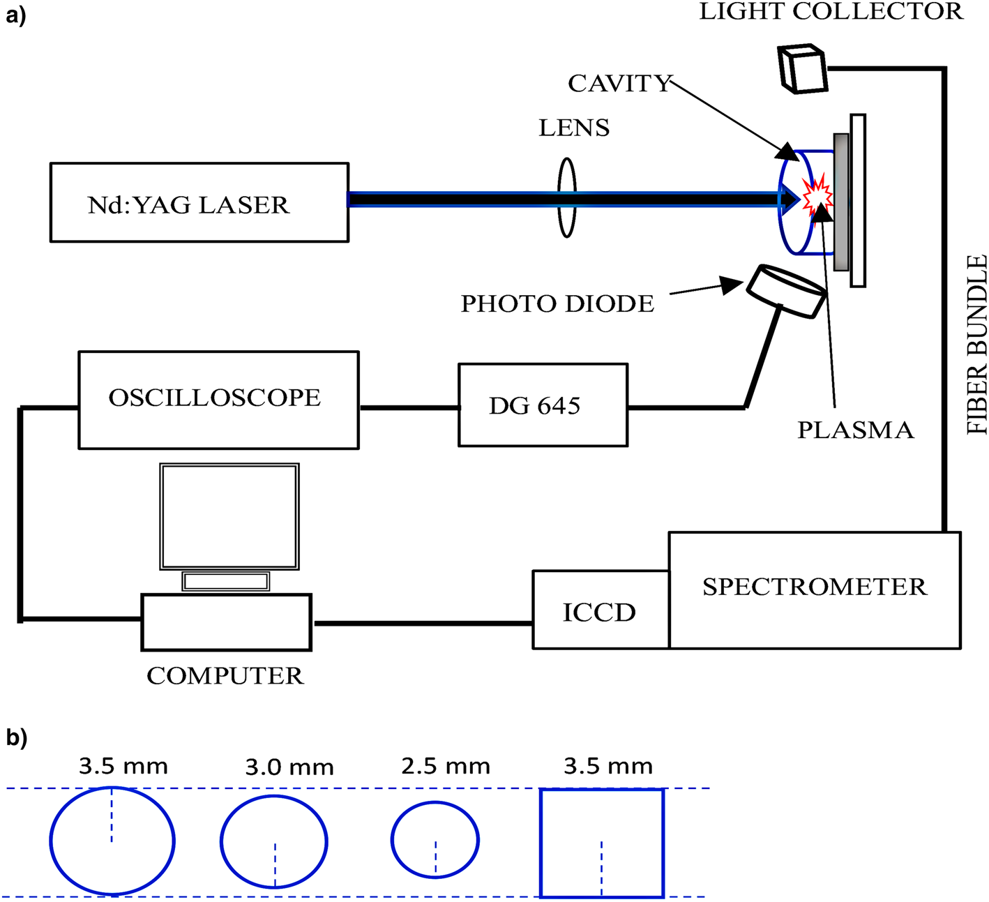
The schematic diagram of the experimental setup is represented in Figure 1a. The experiment was conducted in air under atmospheric pressure. A Q-switched Nd:YAG laser operating at its fundamental wavelength of 1064 nm, with a pulse width of 10 ns, and the repetition rate of 10 Hz was used to ablate the surface of the Mg-target sample (certified purity of 99.99%) to generate the plasma plume. A quartz lens with a focal length of 150 mm was used to focus the laser beam on the surface of the Mg target. We employed laser energies of 200, 300, and 400 mJ, which were measured by a pyrometric detector.

Fig. 1. (a) The schematic diagram of the experiment of the cavity confinement of the laser-induced Mg plasma. (b) Three different circular cavities with radii of 2.5, 3.0, and 3.5 mm and a square cavity with half of its side as 3.5 mm.
The emission spectra from the laser-induced plasmas were collected by a fiber bundle (50-μm core diameter) coupled with a Michelle spectrometer with an inbuilt intensified charged coupled device (ICCD) camera (1024 × 1024 pixels, iStar from Andor Technology). The delay generator (Stanford Research System, model DG645) was utilized to vary the time between the laser pulse and the acquisition of the spectral images. Two different shapes of the columnar cavity were employed for the confinement. The square cavity of side 7 mm (half of the side as 3.5 mm, denoted by R s 3.5 mm) and a circular cavity with three different radii of 2.5, 3.0, and 3.5 mm (indicated by R c 2.5, 3.0, and 3.5 mm, respectively) were used in the experiment as depicted in Figure 1b. The depth of all the cavities was 7 mm. The cavity was tightly fitted to the 3D translation stage to ensure that the laser beam was focused at the center of the cavity. The data acquisition and its analysis were performed with a computer running a manufacturer software (Andor Solis, Andor Technology).
The schematic diagram in Figure 2 is also used to study the magnetic confinement of the laser-induced plasma. The target samples were mounted on an adjustable holder, which was sandwiched between two permanent magnets. The distance between the two magnets was kept constant. The Gauss meter was then used to measure the magnetic field strength of the magnets. The magnetic fields produced by the magnets were utilized in a way that the magnetic field lines were perpendicular to the plasma expansion.
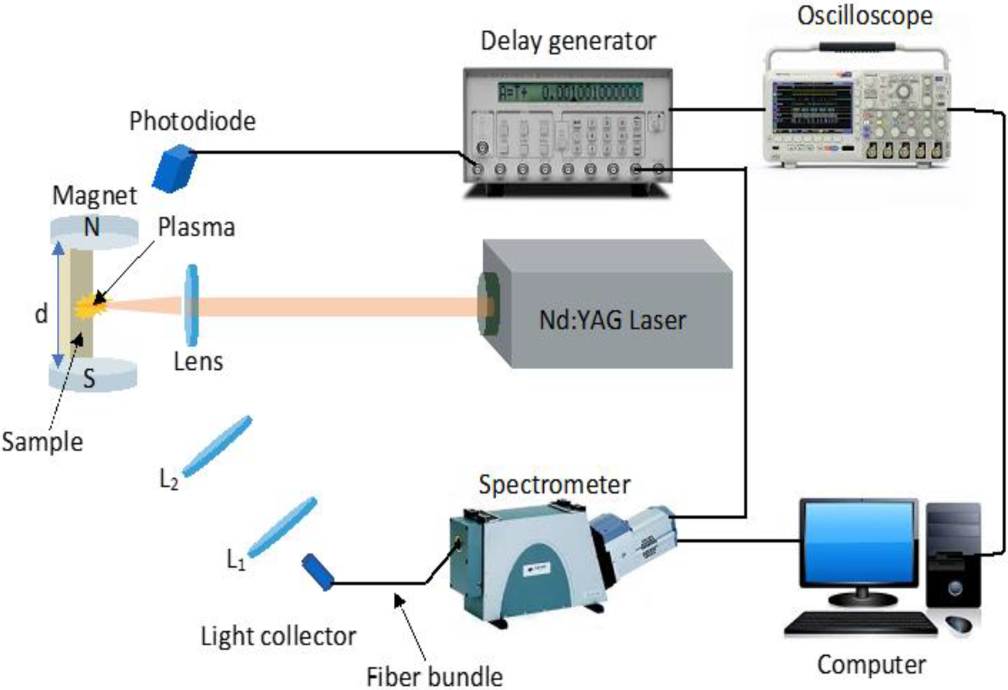
Fig. 2. The schematic diagram of the magnetic confinement of the laser-induced plasma at the atmospheric pressure.
Results and discussion
Cavity confinement
Spectral intensities
The time-integrated laser-induced spectra of the Mg plasma were measured to investigate the influence of the cavity confinement on the signal enhancement of the plasma. The emission spectra of the magnesium plasma recorded with circular cavities with three different radii at the laser energy of 250 mJ were obtained in the spectral ranges of 515.8–519.4 nm, as shown in Figure 3. The Nd:YAG laser beam was focused to a spot size of approximately 0.42 mm in diameter, with a laser energy of 250 mJ and a delay time of 350 ns. The acquisitions of the spectra data were recorded a suitable number of accumulations to increase the signal-to-noise ratio. The emission intensities of the Mg atomic lines were all enhanced in the presence of the circular cavity. The atomic lines of the Mg spectra lines were used from the data compiled from the National Institute for Standards and Technology database (NIST).

Fig. 3. The spectra for different circular cavities of radii (2.5, 3.0, and 3.5 mm) at a delay time of 350 ns and a laser energy of 250 mJ from the spectral range of 515.98–519.32 nm.
Effect of the cavity radii and shape on the plasma
To improve the cavity dimension in this study, we employed the circular cavities of different radii. The emission intensities of the Mg plasma were studied using circular cavities of radii 2.5, 3.0, and 3.5 mm, respectively, as shown in Figure 4. The intensities of the different circular cavity radii were plotted with the cavity-free case (without cavity) for comparison. Comparing the emission intensities of the circular cavity of 2.5 mm radius with the cavity-free case (without cavity), the emission intensity of the Mg I-518.4 nm was slightly enhanced at a delay time of 50 ns. Increasing the delay time to 150 ns, the emission intensity started rising slowly and then increased significantly at a delay time of 200 ns, and this can be as a result of a decrease in the lifetime of the upper state of the Mg plasma due to the confinement. Afterwards, there was a rapid rise in the intensity of the circular cavity of 2.5 mm from 200 to 350 ns. Moreover, the emission intensity then decreases quickly after 350 ns. The highest enhancement of the 2.5 mm cavity radius was found to be approximately 3.8 at a delay time of 350 ns. Similar observations were obtained for the circular cavities of radii 3.0 and 3.5 mm and both obtained their maximum emission intensities at a delay time of 350 ns, reaching an enhancement factor of approximately 3.4 and 2.8, respectively. Comparing all the cavity radii with the cavity-free case (without cavity) as can be seen from Figure 4, the spectral intensities of all the three different cavity confinements were all enhanced. These enhancements resulted from the plasma compression, caused by the shock waves reflected from the walls of the cavities. The enhancement shows that the reflected shock waves have more effect on the Mg plasma plume (Gao et al., Reference Gao, Liu, Song and Lin2015; Wang et al., Reference Wang, Chen, Zhang, Wang, Sui, Li, Jiang and Jin2018). This is because the compression by the shock wave would lead to an increase in the rate of collision between the particles, causing a rise in the number of atoms in high-energy states and thus reheating and keeping a higher temperature within the plasma plume, thereby causing an enhancement in the emission intensity of the Mg plasma (Guo et al., Reference Guo, Hao, Shen, Xiong, He, Xie, Gao, Li, Zeng and Lu2013).

Fig. 4. Time-resolved spectroscopy of Mg I-518.4 nm with different circular cavity radii of 2.5, 3.0, and 3.5 mm and cavity-free case (without cavity) at a laser energy of 350 mJ.
We observed that at a delay time of 350 ns, the size of the ablated plasma was compressed by the reflected shock wave, thereby decreasing the size of the plasma. As a result, the maximum plasma density was attained. With a further increase in the delay time, the compression of the shock wave becomes weaker, and the shock wave propagates through the plasma. When this happens, the volume of the plasma expands; the plasma density then progressively decreases, leading to a decrease in the intensity of the plasma (Wang et al., Reference Wang, Chen, Zhang, Wang, Sui, Li, Jiang and Jin2018).
From our results, we observed that the radius of the cavity had a tremendous effect on the enhancement of the emission intensities, and the circular cavity of radius 2.5 mm had the best confinement.
The spectral peak intensities of Mg I-516.7 nm, Mg I-517.3 nm, and Mg I-518.4 nm with different circular cavities of radii (2.5, 3.0, and 3.5 mm) at a delay time of 350 ns and a laser energy of 300 mJ are depicted in Figure 5. At a delay time of 350 ns and a laser energy of 300 mJ, the peak intensities of the Mg spectral lines confined with a circular cavity of radius 2.5 mm had the strongest emission intensity. We observed that the enhancement factors of the spectral intensities of the Mg I-516.7 nm, Mg I-517.3 nm, and Mg I-518.4 nm spectral lines are higher with the circular cavity of radius 2.5 mm followed by the cavity radius of 3.0 and 3.5 mm.

Fig. 5. The spectral peak intensities for different circular cavity radii (2.5, 3.0, and 3.5 mm) at a delay time of 350 ns and a laser energy of 300 mJ of Mg I-516.7 nm, Mg I-517.3 nm, and Mg I-518.4 nm.
A graph of a circular cavity with a radius 3.5 mm and a square cavity with the length of the side as 7 mm (half of its side as 3.5 mm) is shown in Figure 6. Comparing the square cavity with the cavity-free case (without cavity), we observed a general trend of decreasing spectral intensities with an increasing delay time from 50 to 800 ns with the cavity-free case (without cavity). From the graph in Figure 6, there was no significant increase in the spectral intensities of the square cavity with an increasing delay time from 50 to 150 ns as compared with the cavity-free case (without cavity). The intensities of the square cavity started to increase slowly from a delay time of 200 ns and then increased rapidly to its maximum intensity at a delay time of 350 ns. With a further increase in the delay time to 400 ns, the intensity then drops sharply with increasing the delay time from 450 to 800 ns. Also, the intensity of the circular cavity was more enhanced as compared with the square cavity. The circular cavity attained its highest spectral intensity at a delay time of 350 ns and then decreased rapidly from a delay time of 400–700 ns. There was a slight increase in the intensity of the circular cavity from the delay time of 700–750 ns and then dropped again at a delay time of 800 ns.

Fig. 6. The emission intensity of Mg plasma confined with a circular cavity of radius 3.5 mm (R c 3.5 mm) and a square cavity of half of its side as 3.5 mm (R s 3.5 mm) with different delay time at a laser energy of 250 mJ.
Figure 7 shows the spectral peak intensities of Mg plasma confined with a circular cavity of radius 3.5 mm and a square cavity with half of its side as 3.5 mm at a delay time of 300 ns and a laser energy of 250 mJ with the Mg spectral lines of 516.7, 517.3, and 518.4 nm. The Mg I-518.4 nm attained the highest spectral peak intensity of 22,996. With the same laser energy and delay time, the spectral peak intensity of the square cavity was recorded as 21,578. Also, the cavity-free case (without cavity) recorded the lowest spectral peak intensity of the Mg I-518.4 nm as 15,267 at a delay time of 300 ns and a laser energy of 250 mJ. We observed that the peak intensities of the circular cavity are higher as compared with the square cavity and the cavity-free case (without cavity).

Fig. 7. The spectral peak intensities for the circular cavity of radius 3.5 mm, a square cavity with half of its side as 3.5 mm, and the cavity-free case (without cavity) at a delay time of 300 ns and a laser energy of 250 mJ of Mg I-516.7 nm, MgI-517.3 nm, and Mg I-518.4 nm.
Determination of plasma temperature using the Boltzmann plot method
The electron temperature was obtained by employing the Boltzmann plot method (Aguilera and Aragón, Reference Aguilera and Aragón2004; Zhang et al., Reference Zhang, Wang, He, Jiang, Zhang, Hang and Huang2014; Hongbing et al., Reference Hongbing, Asamoah, Jiawei, Dongqing and Fengxiao2018), which can be expressed as follows:
 $$\ln \left( {\displaystyle{{I_{{\rm mn}}{\rm \lambda}_{{\rm mn}}} \over {A_{{\rm mn}}g_{{\rm mn}}}}} \right) = -\displaystyle{{E_{\rm m}} \over {k_{\rm B}T}} + \ln \left( {\displaystyle{{hcN} \over {U\lpar T \rpar }}} \right)\; $$
where U(T) is the partition function, the subscripts m and n represent the upper energy level of the transition and the lower energy level of the transition, respectively, c is the speed of light (ms−1), E m is the energy of the upper energy level (eV), k B is the Boltzmann's constant (eV K−1), g m is the statistical weight of the upper energy level, λmn is the transition wavelength (m), h is the Planck's constant, N is the number density (m−3), A mn is the transition probability (s−1), and T is the electron temperature (K) (Ahmed et al., Reference Ahmed, Abdullah, Ahmed, Piracha and Baig2017; Figures 8–10).

Fig. 8. The Boltzmann plot using Mg lines at a delay time of 350 ns and a laser energy of 250 mJ.

Fig. 9. The Saha Boltzmann plot using Ti lines at a delay time of 350 ns and a laser energy of 250 mJ.

Fig. 10. The temporal evolution of the electron temperature of the Mg plasma, with different circular cavities (R c 2.5, 3.0, and 3.5 mm) and the cavity-free case (without cavity) at a laser energy of 300 mJ.
Plotting the energies of the upper energy levels (E m) at the right-hand side of Eq. (1) against ln(I mnλmn/A mng mn) at the left-hand side yields a linear plot with slope equal to − 1/k BT. By utilizing the atomic spectral lines of Mg I of wavelength 383.2, 470.3, and 518.4 nm, the temperature can be deduced from the Boltzmann plot using the slope obtained from the plot. The spectroscopic parameters of both the Mg and Ti spectra lines retrieved from the NIST database are shown in Table 1.
Table 1. The spectroscopic data of Mg and Ti spectral lines obtained from the NIST database

Influence of the cavity radii on the electron temperature
The slope of the plot for the cavity-free case (without cavity) yielded an electron temperature of 7423 K at a delay time of 200 ns and a laser energy of 300 mJ. With the same laser energy and delay time, the electron temperature of the circular cavities of radii 2.5, 3.0, and 3.5 mm was recorded at 9188, 8575, and 7683 K, respectively. Comparing the plot of the electron temperature against the delay time, we observed that the electron temperature of the cavity-free case (without cavity) decreases with increasing delay time, and this result agrees with our previous work (Asamoah and Hongbing, Reference Asamoah and Hongbing2017). But, with the circular cavity of radius 2.5 mm, the electron temperature does not follow the usual trend, it started decreasing with increasing delay time from 50 to 200 ns and then began to rise slowly from 250 ns until it attained its highest electron temperature of 15,889 K at a delay time of 350 ns. It then starts to decrease from 400 to 800 ns. The circular cavity of radii 3.0 and 3.5 mm also obtained their highest electron temperatures as 14,843 and 13,833 K, respectively, at a delay time of 350 ns. The cavity confinement had a significant impact on the electron temperature with an enhancement factor of approximately 3.1, 2.6, and 2.3 with circular cavities of radii 2.5, 3.0, and 3.5 mm, respectively.
We also studied the temporal evolution of the electron temperature with three different laser energies (200, 300, and 400 mJ). The results of this study are depicted in Figure 11. We observed that at a delay time of 350 ns and a laser energy of 400 mJ, the circular cavity of radius 2.5 mm had the maximum electron temperature of 16,853 K. The square cavity also obtained its maximum electron temperature of 15,018 K at a delay time of 350 ns and a laser energy of 400 mJ. From Figure 11, it can be seen that the electron temperature increases with increasing laser energy, with the circular cavity of radius 2.5 mm having the highest electron temperature.

Fig. 11. The plot of the electron temperature at a delay time of 350 ns with different laser energies (200, 300, and 400 mJ) against the circular cavities (R c 2.5, 3.0, and 3.5 mm), the square cavity, and the cavity-free case (without cavity).
We further employed a laser energy of 500 mJ to study the temporal evolution of the electron temperature. At a delay time of 350 ns, the electron temperatures of the Mg plasma for the circular cavities of radii 2.5, 3.0, and 3.5 mm were recorded as 18,920, 18,325, and 17,408 K, respectively. The electron temperature increased significantly by increasing the laser energy to 500 mJ as shown in Figure 12. The significant enhancement of the electron temperature occurred between the delay time of 200 and 350 ns. From Figure 13, the electron temperature decreases rapidly with an increasing delay time from 350 to 750 ns with a laser energy of 500 mJ.

Fig. 12. The temporal evolution of the electron temperature of the Mg plasma, with different circular cavities (R c 2.5 mm, 3.0 mm, and 3.5 mm) and the cavity-free case (without cavity) from the delay time of 50–350 ns with a laser energy of 500 mJ.

Fig. 13. The temporal evolution of the electron temperature of the Mg plasma, with different circular cavities (R c 2.5 mm, 3.0 mm, and 3.5 mm) and the cavity-free case (without cavity) from the delay time of 350–750 ns with a laser energy of 500 mJ.
Magnetic confinement
The emission spectra of the Mg and Ti target samples are investigated with and without magnetic fields at several delay times. Figures 14 and 15 depict time-resolved Mg and Ti emission spectra at delay time from 0 to 35 μs, respectively. From Figure 14, the Mg spectra of Mg I-518.4 nm attained the highest spectral intensity of 8927.95. We also observed a drop in the spectral intensities of the Mg lines with increasing delay time. Figure 15 also shows the Ti spectra for both the atomic lines of Ti I: 336.2, 390.1, and 430.1 nm and the ionic lines of Ti II: 337.3, 368.5, 376.2, and 439.5 nm. The Ti II-376.2 nm spectral line reached its maximum spectral intensity at 4569.86 with a delay time of 5 µs at the presence of the magnetic field of 0.47 T. The Mg I-518.4 nm spectral line was fitted to the Lorentz profile in Figure 16, with a laser energy of 50 mJ and a delay time of 25 µs.

Fig. 14. Time-resolved emission spectrum of Mg-induced plasma at several delay times in the spectral region of 200−865 nm with a laser energy of 50 mJ at the presence of a magnetic field of 0.47 T.

Fig. 15. Time-resolved emission spectrum of Ti-induced plasma at several delay times in the spectral region of 300−562 nm with a laser energy of 50 mJ at the presence of a magnetic field of 0.47 T.

Fig. 16. The Lorentz fit of the Mg I-518.4 nm line with a delay time of 25 µs and a laser energy of 50 mJ at the presence of a magnetic field of 0.47 T.
The enhancements of the spectral intensities of the laser-induced plasmas are attributed to the magnetic confinement effect. By applying external magnetic fields, the Lorentz force would significantly influence the ions and electrons within the produced plasmas, thereby reducing the propagation of the ablated plume. Also, other phenomena are introduced at the presence of the applied magnetic field such as the conversion of kinetic energy into plasma thermal energy and plume confinement. However, the magnetic field cannot entirely stop the propagation of the ablated plume; hence, the ablated plume propagates slowly through the magnetic field (Joshi et al., Reference Joshi, Kumar, Singh and Prahlad2010; Iftikhar et al., Reference Iftikhar, Bashir, Dawood, Akram, Hayat, Mahmood, Zaheer, Amin and Murtaza2017). Using the magnetohydrodynamic equation, the parameter β can be deduced by the following equation (Harilal et al., Reference Harilal, Tillack, O'shay, Bindhu and Najmabadi2004; Shen et al., Reference Shen, Lu, Gebre, Ling and Han2006):
 $${\rm \beta} = \displaystyle{{8{\rm \pi} n_{\rm e}k_{\rm B}T_{\rm e}} \over {B^2}} = \displaystyle{{{\rm Plasma}\;{\rm pressure}} \over {{\rm Magnetic}\;{\rm pressure}}}\; $$
where T e, n e, and k B are the electron temperature, number density, and Boltzmann constant, respectively, β is the ratio of the plasma pressure and the magnetic pressure, and B is the magnetic field strength (Rai et al., Reference Rai, Shukla and Pant1998; Iftikhar et al., Reference Iftikhar, Bashir, Dawood, Akram, Hayat, Mahmood, Zaheer, Amin and Murtaza2017). At the presence of the magnetic field, the deceleration of the ablated plasma expansion can be expressed as follows:
 $$\; \displaystyle{{{\rm v}_2} \over {{\rm v}_1}} = \left( {1-\displaystyle{1 \over {\rm \beta}}} \right)^{(1/2)}$$
where v2 and v1 represent the asymptotic plasma expansion velocity with and without a magnetic field, respectively. When β = 1, the ablated plasma would be stopped entirely by the magnetic field; this shows that the magnetic pressure is equal to the thermal pressure. If β > 1, the magnetic confinement would be ineffective. However, if β < 1, then magnetic confinement becomes effective (Shen et al., Reference Shen, Lu, Gebre, Ling and Han2006; Iftikhar et al., Reference Iftikhar, Bashir, Dawood, Akram, Hayat, Mahmood, Zaheer, Amin and Murtaza2017; Akhtar et al., Reference Akhtar, Jabbar, Ahmed, Mehmood, Umar, Ahmed and Baig2019). From all the calculations of β in all the cases, we found that the value of β was less than 1, which confirms that there was plasma confinement at the presence of the magnetic field.
Employing a magnetic field of 1.23 T and a laser energy 450 mJ in Figure 17, the Mg I-518.4 nm spectral line intensity increases from a delay time of 1–4 µs. We observed the highest intensity of the Mg I-518.4 nm spectra at 23,880 with a delay time of 4 µs. The intensity then drops tremendously from a delay time of 5–32 µs. The magnetic field of 0.62 and 0.91 T also attained their maximum intensities at a delay time of 2 µs and then decreased from the delay time of 3–32 µs. Also, reducing the magnetic field strength to 0.47 T, the intensity of the Mg I-518.4 nm line reached its maximum intensity at a delay time of 4 µs and then decreased.

Fig. 17. The intensities of the Mg I-518.4 nm spectra line against the delay times, with a laser energy of 450 mJ at the presence and absence of the magnetic field.
For the Ti II-376.2 nm spectra lines in Figure 18, the maximum spectral intensity was reached at the delay time of 2 µs at the presence of the magnetic field 1.23 T. The Ti II-376.2 nm spectra lines also had a decreasing trend with an increasing delay time from 4 to 32 µs.

Fig. 18. The intensities of the Ti II-376.2 nm spectra line against the delay times, with a laser energy of 450 mJ at the presence and absence of the magnetic field.
Plotting the spectral intensities of both the Mg and Ti plasmas against the laser energies is represented in Figures 19 and 20, respectively. The intensities of the Mg plasma in Figure 19 increased with an increasing laser energy from 50 to 350 mJ at the presence and absence of the magnetic field of 0, 0.47, 0.62, 0.91, and 1.23 T. Also, from Figure 20, the spectral intensities of the Ti plasma predicted a general trend of increasing intensities with increasing laser energy at the presence and absence of the magnetic fields.

Fig. 19. A plot of the intensities of the Mg I-518.4 nm spectra line against the laser energies at the presence and absence of the magnetic field.

Fig. 20. A plot of the intensities of the Ti II-376.2 nm spectra line against the laser energies at the presence and absence of the magnetic field.
Saha-Boltzmann plot method
Considering the ionic and the neutral lines of the Ti spectra, the Saha-Boltzmann plot method can be employed to determine the plasma temperatures of the laser-induced Ti plasmas. The neutral and the ionic lines can be expressed in Eqs. (4) and (5), respectively:
 $${\rm ln}\left( {\displaystyle{{I_1{\rm \lambda}_1} \over {g_1A_1}}} \right) = -\displaystyle{1 \over {kT}}E_k^1 + {\rm ln}\left( {{hc}\displaystyle{{N_0} \over {Z_0\lpar T \rpar }}} \right)\; $$
 $${\rm ln}\left( {\displaystyle{{I_2{\rm \lambda}_2} \over {g_2A_2}}} \right)-{\rm ln}\left( {\displaystyle{{2\lpar {2 {\rm \pi} mk} \rpar \lpar {3/2} \rpar } \over {h^3}}\displaystyle{{T^{3/2}} \over {N_{\rm e}}}} \right) = -\displaystyle{1 \over {kT}} \times \lpar {E_{\rm k}^2 + E_{{\rm IP}}} \rpar + {\rm ln}\left( {hc\displaystyle{{N_0} \over {Z_0\lpar T \rpar }}} \right)$$
where the subscripts 1 and 2 represent the neutral and the ionic lines, respectively. m is the mass of the electron (kg), c is the speed of light, Z 0(T) denotes the partition function, E IP is the ionization energy (eV), A is the transition probability, T is the plasma temperature (K), N 0 is the particle density of the element, and N e is electron density (m−3) (Griem, Reference Griem1997; Gomba et al., Reference Gomba, D'Angelo, Bertuccelli and Bertuccelli2001; Duixiong et al., Reference Duixiong, Maogen, Chenzhong and Guanhong2014).
Equation (5) can be reduced to the Boltzmann plot equation by expressing the energies  $E_{\rm k}^1$ and
  $E_{\rm k}^* = E_{\rm k}^2 + E_{{\rm IP}}$ for both the neutral and the ionic lines, respectively. We obtain a reduced form of Eq. (5) as follows:
 $${\rm ln}\left( {\displaystyle{{I_1{\rm \lambda}_1} \over {g_1A_1}}} \right)^{^\ast} = -\displaystyle{1 \over {kT}}E_{\rm k}^{^\ast} + {\rm ln}\left( {hc\displaystyle{{N_0} \over {Z_0\lpar T \rpar }}} \right)\; $$
From the Boltzmann plot, the electron temperatures of the Mg plasma at a delay time of 5 µs and a laser energy of 250 mJ were found to be 7428, 9643, 11,038, and 12,618 K, which correspond to the magnetic fields of 0, 0.43, 0.62, and 0.91 T, respectively. From Figure 21, the electron temperature of the Mg plasma recorded its highest electron temperature of 14,591 K with a laser energy of 300 mJ and a delay time of 10 µs at the presence of a magnetic field of 1.23 T. The error bars in the figure show the standard deviations in calculating the electron temperatures.

Fig. 21. A plot of electron temperature of Mg plasma against laser energy, with a delay time of 20 µs at the presence and absence of magnetic fields of 0, 0.47, 0.62, 0.91, and 1.23 T.
The Saha-Boltzmann plot method was also used to determine the electron temperature of the Ti plasma. The slope of the plot gave an electron temperature of 6085, 7045, 8012, 9078, and 9987 K with a delay time of 5 µs at the presence and absence of magnetic fields of 0, 0.47, 0.62, 0.91, and 1.23 T, respectively. The highest electron temperature of the Ti plasma was recorded to be 15,720 K at a delay time of 10 µs. We also observe a sharp increase in the electron temperature with increasing laser energy at the presence of a magnetic field of 1.23 T. Figure 22 shows a plot of the electron temperature of Ti plasma against the laser energy, with a delay time of 20 µs.

Fig. 22. A plot of electron temperature of Ti plasma against laser energy, with a delay time of 20 µs at the presence and absence of magnetic fields of 0, 0.47, 0.62, 0.91, and 1.23 T.
Electron density
In this section, we further evaluate the electron density from the Stark broadening mechanism. The line profiles of the Mg and the Ti lines are fitted to the Lorentzian fit as depicted in Figure 16. The full width at half maximum of the spectral lines can be used to evaluate the electron number density by the relation (Sun et al., Reference Sun, Su, Dong, Wen and Cao2013; Asamoah and Hongbing, Reference Asamoah and Hongbing2017; Ghezelbash et al., Reference Ghezelbash, Majd, Darbani and Ghasemi2017):
 $${\rm \Delta} {\rm \lambda} _{1/2}\lpar {{\rm nm}} \rpar = 2{\rm \omega} \left( {\displaystyle{{N_{\rm e}} \over {{10}^{16}}}} \right) + 3.5\;{A}\left( {\displaystyle{{N_{\rm e}} \over {{10}^{16}}}} \right)^{1/4}\left[ {1-\displaystyle{3 \over 4}N_{\rm D}^{-1/3}} \right]{\rm \omega} \left( {\displaystyle{{N_{\rm e}} \over {{10}^{16}}}} \right)\; $$
where N e is the electron density, A is the ionic broadening parameter (nm), ω is the electron impact width parameter (nm), and N D denotes the number of particles in the Debye sphere. Neglecting the ionic broadening from Eq. (7), due to its minor contribution to the broadening, hence, Eq. (7) can be reduced to the form:
 $${\rm \Delta} {\rm \lambda} _{1/2}\lpar {{\rm nm}} \rpar = 2{\rm \omega} \left( {\displaystyle{{N_{\rm e}} \over {{10}^{16}}}} \right)$$
Figures 23 and 24 show the plot of electron density against the laser energy of Mg and Ti, respectively, at the presence and absence of magnetic field. The electron density was deduced from the stark broadening at the presence and absence of the magnetic field. In the absence of the magnetic field, the electron density of the Mg plasma was found to be in the range from 1.03 × 10¹⁸ to 1.68 × 1018 cm−3 with varying laser energy from 50 to 350 mJ. At the presence of the magnetic fields of 0.47, 0.62, 0.91, and 1.23 T, the electron density was found to be in the range of 1.14 × 10¹⁸−1.81 × 10¹⁸, 1.28 × 10¹⁸−1.92 × 10¹⁸, 1.42 × 10¹⁸−2.03 × 10¹⁸, and 1.55 × 10¹⁸−2.14 × 1018 cm−3, respectively, with varying laser energy from 50 to 350 mJ.

Fig. 23. A plot of electron density of Mg plasma against laser energy, with a delay time of 15 µs at the presence and absence of magnetic fields of 0, 0.47, 0.62, 0.91, and 1.23 T.

Fig. 24. A plot of electron density of Ti plasma against laser energy, with a delay time of 15 µs at the presence and absence of magnetic fields of 0, 0.47, 0.62, 0.91, and 1.23 T.
The electron density of the Ti plasma was found in the range of 0.97 × 10¹⁸−1.53 × 1018 cm−3 at the absence of the magnetic field. And with an applied magnetic field of 0.47, 0.62, 0.91, and 1.23 T, the electron densities of the Ti plasma were found to be in the range of 1.07 × 10¹⁸−1.65 × 10¹⁸, 1.13 × 10¹⁸−1.72 × 10¹⁸, 1.26 × 10¹⁸−1.83 × 10¹⁸, and 1.33 × 10¹⁸−1.89 × 1018 cm−3, respectively.
We recorded an increasing trend of the electron density with an increasing magnetic field. The electron density shows that the energy transfer within the plasma plume and the collisions significantly increased with the applied magnetic field, hence increasing both the electron temperature and the electron density.
Validity of the LTE
For an accurate and precise analysis of the qualitative and quantitative study of the elemental composition of target samples, it is imperative to establish the validity of Local Thermodynamic Equilibrium (LTE) and also determine that the plasma of the sample is optically thin. Failure to warrant the existence of LTE conditions might lead to incorrect and unreliable measurements as a result of intense self-absorption of the plasma.
McWhirter's criterion (Sabsabi and Cielo, Reference Sabsabi and Cielo1995) should be fulfilled before LTE can be established. The criterion is based on the fact that the collision rate of the electrons should be more than that of the radiation rate. When this case happens, the plasma is classified to be in LTE. The criterion requires a certain amount of electron number density to be present for LTE to be ascertained, which can be expressed mathematically as follows (Aguilera and Aragón, Reference Aguilera and Aragón2004; Dawood and Bashir, Reference Dawood and Bashir2018):
 $$N_{\rm e} \ge 1.6 \times 10^{12}T^{1/2}\lpar {{\rm \Delta} E} \rpar ^3$$
where T is the plasma temperature (K) and ΔE is the energy difference between the transition levels of the upper and lower energy levels of both the Mg and Ti lines under investigation. When the evaluated electron number density, from the experiment using the Stark broadening of the atomic and ionic lines, is higher than the electron number density estimated from the McWhirter's criterion, then we can establish that the plasma is said to be in LTE. Several research works have proved that McWhirter's criterion is not a sufficient method to ascertain the existence of LTE. From this work, we evaluated the electron density from the temperatures of the Mg and Ti plasmas, and the electron density was found to be in the order of 1018 cm−3 which was high enough to affirm the existence of LTE. Also, we established that the plasma was optically thin from the line intensities obtained and chosen for the calculation of the plasma temperatures.
Conclusion
The influence of cavity and magnetic confinement on the signal enhancement of laser-induced Mg and Ti plasmas generated by a Q-switched Nd:YAG laser is studied. The circular and square cavities were used to confine the plasma plume. We found that there was a significant enhancement in the spectral intensities of the three different circular cavity radii as compared with the cavity-free case. The maximum enhancement factor of the Mg I-518.4 nm line was reached at approximately 3.8, 3.4, and 2.8 at a delay time of 350 ns and a laser energy of 350 mJ for circular cavities of radii 2.5, 3.0, and 3.5 mm, respectively. Comparing the circular cavity of radius 3.5 mm with the square cavity at a delay time of 300 ns and a laser energy of 300 mJ, the intensity of the circular cavity was more enhanced as compared to the square cavity. The value for the electron temperature for the cavity-free case (without cavity) was found to be 7423 K at a delay time of 200 ns and a laser energy of 300 mJ. With the same experimental conditions, the electron temperature of the circular cavities of radii 2.5, 3.0, and 3.5 mm was recorded at 9188, 8575, and 7683 K, respectively. At the presence of the magnetic field, we also observed a tremendous effect on the electron temperature and density. The value of the electron temperatures of Mg and Ti plasmas recorded their highest electron temperatures of 14,591 and 15,720 K with a laser energy of 300 mJ and a delay time of 10 µs at the presence of magnetic field of 1.23 T. Varying the magnetic field from 0.47 to 1.23 T, the temperature of the plasma increased significantly, and this was attributed to the adiabatic compression and Joule heating. The electron density of Mg and Ti plasmas at the presence of the magnetic field of 1.23 T was found to be in the range of 1.55 × 10¹⁸−2.14 × 10¹⁸ and 1.33 × 10¹⁸−1.89 × 1018 cm−3, respectively. From our calculations, the value of β, which was less than 1 for all the cases, confirms that there was a plasma confinement at the presence of the magnetic field.
Acknowledgments
This work was supported by the National Natural Science Foundation of China (Nos. 51775253 and 61505071), the Fundamental Research Funds for the Central Universities (No. 2019B02614), and China Postdoctoral Science Foundation (2017M611725).