


NOMENCLATURE
- A, B
-
constants
-
 $\overrightarrow{A},\overrightarrow{B}$
-
arbitrary vectors
- CFL
-
Courant-Friedrichs-Lewy
- C D
-
coefficient of drag
- DPM
-
Discrete Particle Model
- D p
-
droplet diameter
- E m
-
mass fraction of splashed droplets relative to the impacting droplet
- F
-
force
- F d , F n , f
-
droplet train frequency
- F D
-
drag force
- F s
-
surface tension force
- g
-
gas phase, gravity
- h*
-
relative film thickness
- h
-
grid spacing
- h film , R w
-
film thickness
- H* x , H* f
-
geometry dimension relative droplet diameter
- H ε
-
Heaviside function
- H x , H y , H z
-
geometry dimension
- K
-
splash factor
- La
-
Laplace number
-
$\dot{m}_p$
-
mass flow rate of droplet
- M
-
inter-phase mass exchange
- M p
-
mass of a droplet particle before impact
- M s
-
mass of a droplet particle splashing
- N s
-
number of splashing droplets
- N x , N y , N z , N f
-
number of nodes
- Oh
-
Ohnesorge number
- p
-
pressure
- P
-
3D spatial position
- Re
-
Reynolds number
- R s , R
-
actual radius occupied by a droplet continuum
- S, S α, S m
-
source terms
- S*
-
droplet size relative to grid spacing
- t
-
flow time
- U, u
-
velocity (continuum)
- U p , U o
-
droplet velocity
- V cell
-
volume of a computational cell
- VoF
-
volume of fluid
- We
-
Weber number
- X c
-
centroid of a cell
- X p
-
particle position
- ν
-
kinematic viscosity
- σ
-
surface tension
- ρ
-
density
- μ
-
dynamic viscosity
- α
-
volume fraction
- Λ
-
a fluid property
- ϕ
-
level set function
- κ
-
curvature
- δ, δ z
-
delta function
- ε
-
very thin layer
- Δt
-
flow time step
- l
-
liquid phase
- m
-
mass
- o
-
before impact


Greek Symbol
Subscripts
1.0 INTRODUCTION
In specialised engineering applications, liquids can be encountered in different forms – as well-formed droplets or as a well-defined continuum such as film on wall or as a sheet or jets of the liquid. The morphology of the liquid is determined by the interaction of the gas phase and physical properties such as surface tension and viscosity. Oil, for example, is used for lubrication and cooling. Atomising the oil provides a large volume to surface area ratio to convey a high heat flux. In internal combustion engines, atomised engine oil is sprayed to the cylinder walls below the piston area to lubricate the piston-cylinder rubbing. In aeroengines, oil is used to lubricate high speed ball bearings. In this type of application, the oil becomes atomised as it leaves the bearings(Reference Adeniyi, Morvan and Simmons1). In these applications, it is easy to visualise that the atomised oils eventually form a continuum after impact. The continuous oil film can be collected for a reuse. This work is motivated from such applications that involve droplet interaction with and formation of a continuous film. The ability to model such interaction efficiently is therefore key and a CFD model to do so is presented in this paper.
Droplets can also be formed by stripping off from the free liquid surface as a result of Raleigh-Taylor instabilities(Reference Maroteaux, Llory, Coz and Habchi2) or by thin film navigating a sharp bend(Reference Owen and Ryley3) or from ligament breakup(Reference Shinjo and Umemura4). Upon impact of droplets on a dry or pre-wetted wall, secondary droplets (splash) can be formed depending on the impact parameters(Reference Yarin5). Droplet to film interaction is of great engineering interest and has been widely researched, starting with Reynolds’s(Reference Bisighini6) experiment in 1875; although, overall, only a few impact scenarios, such as impact on a gentle film, have been investigated. Other relevant scenarios such as the oblique angle droplet impact on arbitrary moving film on a surface or filaments suspended in space are still lacking. This area of research remains very active, aided with advances in camera technology and wide areas of application to technologies(Reference Marengo, Carlo, Llia V and Cameron7). Modelling is getting more and more relevant for understanding a design. Upon impact of a droplet on a wetted or dry surface, there are a number of possible outcomes, respectively named stick, spread, rebound or splash, as described by Yarin(Reference Yarin5). The trampoline behaviour is a newer regime reported by Bisighini(Reference Bisighini6) in which the free surface deforms like a trampoline after droplet impact. The normal-impact of single droplet on dry and pre-wetted surface was studied by(Reference Brutin8-Reference Sikalo, Marengo, Tropea and Ganic12); others did the impact of a drop train on a heated surface(Reference Cossali, Marengo and Santini13). There are only a few publications on oblique impact, where the droplet had impact at some oblique angle to the surface such as in
![]() ikalo et al(Reference Sikalo, Tropea and Ganic14).
ikalo et al(Reference Sikalo, Tropea and Ganic14).
As the interest in droplet to film experiments is still on-going, so is the modelling of this phenomenon. The free-interface tracking Volume-of-Fluid (VoF) based Computational Fluid Dynamics (CFD) techniques have been successfully used to model both the droplet and the film by fully resolving each droplet onto a CFD mesh grid such as what was done in the work of Riever and Frohn(Reference Rieber and Frohn15) and Peduto et al(Reference Peduto, Koch, Morvan, Dullenkopf and Bauer16), for example. The VoF model was originally proposed by Hirt and Nichols(Reference Hirt and Nichols17) for numerically treating fluid boundaries embedded in a computational cell. It is a relatively affordable way of dealing with segregated flows. VoF is indeed a homogenous Eulerian approach that assumes a single fluid continuum of varying properties defined by so called ‘colour functions,’ typically the volume fractions. It is common to define the interface as the iso-surface of a volume fraction of 50%. Using the volume fraction to define the segregated interface between fluid regions is fine for most computations.
Using the volume fraction in the computation of the surface curvature, however, in the commonly used Brackbill surface tension model(Reference Brackbill, Kothe and Zemach18) can result in over-prediction of the surface tension force. This can, for example, lead to unphysical dry outs(Reference Robinson19). Osher and Sethian(Reference Osher and Sethian20) have defined the interface using a signed continuous Level Set (LS) function. The free interface is here defined as the zero iso-surface of the LS function. The LS function(Reference Sussman and Puckett21) provides a better interface curvature prediction although LS on its own possesses poor mass conservation(Reference Sethian and Smereka22,Reference Son and Hur23) . Bourlioux(Reference Bourlioux24) was first to propose the coupling of both LS and VoF, otherwise called Coupled Level Set Volume of Fluid (CLSVoF). The CLSVoF technique serves to correct for such over-prediction in surface tension, for example, in flows past obstacles and where surface tension is significant(Reference Tkaczyk and Morvan25).
It is possible to simulate the impact and the post-impact outcome of droplets interacting with walls and film using VoF techniques by fully resolving the flow using very fine mesh elements but this can be computationally very expensive; for example, Peduto et al(Reference Peduto, Koch, Morvan, Dullenkopf and Bauer16) used over 3 million computational cells to resolve a single droplet splash. In a multiple droplet impact scenario, fully resolving the droplets to the mesh grid is computationally expensive and may not be practical for a complex engineering configuration. Alternative techniques that are computationally affordable are therefore desirable. A method proposed in this work is to employ the Lagrangian tracking technique to the droplets, whereas, the film and gas phases are treated using the Eulerian VoF technique. Such approach is also known as the Discrete Particle Model or DPM in ANSYS-Fluent which is used to support the work presented in this paper. The two-way interaction between the DPM droplets and the gas phase is achieved by coupling the Lagrangian and Eulerian phases through drag force terms. The coupling of the three numerical components (air, oil-film & oil-droplet), and in particular the (liquid) droplets with the liquid film and or filaments, is achieved by managing source terms in the governing equations. This method requires free-surface tracking and also to determine when a liquid droplet (DPM) is going to interact with the liquid phase in VoF. Existing works(Reference Rieber and Frohn15,Reference Peduto, Koch, Morvan, Dullenkopf and Bauer16) have shown that without using a very fine mesh it is impossible to resolve such phenomenon as droplet splash. From experimental observations(Reference Cossali, Coghe and Marengo10,Reference Mundo, Sommerfeld and Tropea26,Reference O’Rourke and Amsden27) , correlations exist to characterise the splashing of droplets. Conventionally, the primary droplet is the droplet approaching the film and the splashing droplets are often referred to as children or secondary droplets. Correlations from such works inform the creation of child droplet products, where applicable.
The commercial solver, ANSYS-Fluent 14.5 is employed in the present work. The interaction between DPM and Eulerian-VoF is available in ANSYS-Fluent, but coupling of the DPM (which is physically the liquid phase) to the liquid component of VoF, to the authors' knowledge and as proposed here, is new. The technique is numerically checked for mass and momentum conservation. Momentum conservation is checked using the crater evolution of a single drop impact on a film against simulation and correlations from the literature(Reference Cossali, Coghe and Marengo10,Reference Rieber and Frohn15,Reference Okawa, Shiraishi and Mori28,Reference Yarin and Weiss29) . For ease of computation, the film thickness, h*, has been used to describe dry walls (h* = 0), thin film (0 < h* < 1), intermediate film (h* = 1) and deep pools (h* ≫ 1). In this work, a Lagrangian representation is also proposed to continue tracking splashing secondary droplets where experimental correlations are available for such impact regime.
2.0 FORMULATING THE DPM-CLSVoF METHOD
The impact sequence assumes that the droplet is firstly in the gas phase and travels towards a wall or a film. The droplet hits the film interface or a dry wall. At low impact energies, the droplets become part of the film and do not create extra child droplets. At high energy impact, child droplets are formed after absorbing part of the primary droplet. We should be able to predict the free film interface, track the primary droplet in the gas phase and its impact onto the film, as well as create the splashed children numerically.
The Navier-Stokes and continuity equations formulation for incompressible flow, respectively, given in Equations (1) and (2) are employed. The Navier-Stokes equations represent the force balance at each point in the domain. The inertial terms are balanced with the divergence of stress, body forces and other contributory source terms such as
 $\overrightarrow{S_m}$
.
$\overrightarrow{S_m}$
.
 $$\begin{eqnarray}
&& \overbrace{\rho \left( \overbrace{\frac{\partial \overrightarrow{\vphantom{U}u}}{\partial t}}^{\text{ unsteady acceleration}} + \underbrace{\nabla \cdot \left( \overrightarrow{\vphantom{U}u} \overrightarrow{\vphantom{U}u} \right) }_{ \text{ convective acceleration}} \right)}^{\text{ Inertial terms}} \nonumber \\
&& = \overbrace{-\underbrace{\nabla p}_{\text{ pressure gradient}}+\underbrace{\nabla \cdot \mu \left[ \nabla \overrightarrow{\vphantom{U}u} + \left( \nabla \overrightarrow{\vphantom{U}u} \right)^T \right]}_{\text{ viscous forces}}}^{\text{ Divergence of stress terms}} - \overbrace{F_s + \underbrace{\rho \overrightarrow{\vphantom{G}g}}_{\text{ gravity}}}^{\text{ body forces}} + \underbrace{\overrightarrow{S_m}}_{\text{ source term}}
\end{eqnarray}$$
$$\begin{eqnarray}
&& \overbrace{\rho \left( \overbrace{\frac{\partial \overrightarrow{\vphantom{U}u}}{\partial t}}^{\text{ unsteady acceleration}} + \underbrace{\nabla \cdot \left( \overrightarrow{\vphantom{U}u} \overrightarrow{\vphantom{U}u} \right) }_{ \text{ convective acceleration}} \right)}^{\text{ Inertial terms}} \nonumber \\
&& = \overbrace{-\underbrace{\nabla p}_{\text{ pressure gradient}}+\underbrace{\nabla \cdot \mu \left[ \nabla \overrightarrow{\vphantom{U}u} + \left( \nabla \overrightarrow{\vphantom{U}u} \right)^T \right]}_{\text{ viscous forces}}}^{\text{ Divergence of stress terms}} - \overbrace{F_s + \underbrace{\rho \overrightarrow{\vphantom{G}g}}_{\text{ gravity}}}^{\text{ body forces}} + \underbrace{\overrightarrow{S_m}}_{\text{ source term}}
\end{eqnarray}$$
 $$\begin{equation}
\nabla {\cdot \overrightarrow{\vphantom{U}u} }= 0,
\end{equation}$$
$$\begin{equation}
\nabla {\cdot \overrightarrow{\vphantom{U}u} }= 0,
\end{equation}$$
where F s is the surface tension force added as a spatially varying body force and only near the free surface.
2.1 CLSVoF
The VoF technique is essentially solving the continuity equation for the volume fraction of the present phases in the form of Equation (3).
 $$\begin{equation}
\frac{\partial }{\partial t} \left( \alpha _i \rho _i \right) + \nabla \cdot \left( \alpha _i \rho _i u_i \right) = S_{\alpha _i} + M_{net},
\end{equation}$$
$$\begin{equation}
\frac{\partial }{\partial t} \left( \alpha _i \rho _i \right) + \nabla \cdot \left( \alpha _i \rho _i u_i \right) = S_{\alpha _i} + M_{net},
\end{equation}$$
where M net is the net mass exchange within the phases such as those that may be obtained during evaporation or condensation. Physical phase change is not modelled in this work, thus M net is zero. S α i is the source term. The primary phase volume fraction is not computed using Equation (3), but rather restricted to conserve mass using Equation (4). For a liquid and gas multiphase flow, where the air phase is taken as the primary phase, for example, α l = 1 − α g .
 $$\begin{equation}
\sum _{i=1}^{n} \alpha _i=1
\end{equation}$$
$$\begin{equation}
\sum _{i=1}^{n} \alpha _i=1
\end{equation}$$
The LS function, ϕ, is advected using Equation (5). The LS function, ϕ, can take positive and negative values; the interface is described at the zero LS and the liquid phase is described with positive LS function values.
 $$\begin{equation}
\frac{\partial \phi }{\partial t} + u \cdot \nabla \phi =0
\end{equation}$$
$$\begin{equation}
\frac{\partial \phi }{\partial t} + u \cdot \nabla \phi =0
\end{equation}$$
The equation will move the zero LS exactly as the free-surface motion from the initially known position of the film. The LS function is smooth and continuous; this makes it possible to accurately compute the spatial gradients. This capability of the LS method provides a good estimation of the interface curvature, Equation (6), and in turn, the surface tension force, Equation (7), required in the Navier-Stokes Equation (1).
 $$\begin{equation}
\kappa \left( \phi \right) = \left. \nabla \cdot \frac{\nabla \phi }{\left| \nabla \phi \right|} \right|_{\phi =0}
\end{equation}$$
$$\begin{equation}
\kappa \left( \phi \right) = \left. \nabla \cdot \frac{\nabla \phi }{\left| \nabla \phi \right|} \right|_{\phi =0}
\end{equation}$$
 $$\begin{equation}
F_s = \sigma \kappa \left( \phi \right) \nabla \phi \delta _\varepsilon \left( \phi \right),
\end{equation}$$
$$\begin{equation}
F_s = \sigma \kappa \left( \phi \right) \nabla \phi \delta _\varepsilon \left( \phi \right),
\end{equation}$$
where δε (Equation (8)) is a delta function, smoothed over a distance ε, this is by assuming that the interface can be considered as a ‘thin’ fluid region with a thickness ε.
 $$\begin{equation}
\delta _\varepsilon \left( \phi \right) = \left\lbrace \begin{array}{l@{\quad}l}\frac{1}{2\varepsilon } \left(1+ \cos \left(\frac{\pi \phi }{\varepsilon } \right) \right) & \text{if } \left| \phi \right| < \varepsilon \\
0 & {\rm otherwise} \end{array} \right.,
\end{equation}$$
$$\begin{equation}
\delta _\varepsilon \left( \phi \right) = \left\lbrace \begin{array}{l@{\quad}l}\frac{1}{2\varepsilon } \left(1+ \cos \left(\frac{\pi \phi }{\varepsilon } \right) \right) & \text{if } \left| \phi \right| < \varepsilon \\
0 & {\rm otherwise} \end{array} \right.,
\end{equation}$$
where ε is taken as 1.5 times the grid spacing.
In LS method(Reference Sussman and Puckett21), the effective density and viscosity of the fluid are calculated using Equations (9a) and (9b), respectively.
 $$\begin{eqnarray}
\rho =\rho _g + \left( \rho _l - \rho _g\right)H_\varepsilon \left( \phi \right)
\end{eqnarray}$$
$$\begin{eqnarray}
\rho =\rho _g + \left( \rho _l - \rho _g\right)H_\varepsilon \left( \phi \right)
\end{eqnarray}$$
 $$\begin{eqnarray}
\mu =\mu _g + \left( \mu _l - \mu _g\right)H_\varepsilon \left( \phi \right),
\end{eqnarray}$$
$$\begin{eqnarray}
\mu =\mu _g + \left( \mu _l - \mu _g\right)H_\varepsilon \left( \phi \right),
\end{eqnarray}$$
where H ε(ϕ) is a smoothed Heaviside function.
 $$\begin{equation}
H_\varepsilon \left( \phi \right) = \left\lbrace \begin{array}{l@{\quad}l}0 & \text{if }\phi < -\varepsilon \\
\frac{\left(\phi + \varepsilon \right)}{\left(2\varepsilon \right)} +\frac{1}{\left(2 \pi \right)}{\rm sin} (\frac{\pi \phi }{\varepsilon }) & \text{if }\left| \phi \right| \le \varepsilon \\
1 & \text{if } \phi > \varepsilon \end{array} \right.
\end{equation}$$
$$\begin{equation}
H_\varepsilon \left( \phi \right) = \left\lbrace \begin{array}{l@{\quad}l}0 & \text{if }\phi < -\varepsilon \\
\frac{\left(\phi + \varepsilon \right)}{\left(2\varepsilon \right)} +\frac{1}{\left(2 \pi \right)}{\rm sin} (\frac{\pi \phi }{\varepsilon }) & \text{if }\left| \phi \right| \le \varepsilon \\
1 & \text{if } \phi > \varepsilon \end{array} \right.
\end{equation}$$
The LS function is smooth and continuous; this makes it possible to accurately compute its spatial gradients. This capability of the LS method provides a good estimation of the interface curvature, and in turn, the surface tension force in Equation (1). LS alone is, however, not mass conservative. In the VoF formulation, there is discontinuity at the free surface, posing a weakness for the method to compute the spatial gradients. A major strength of the VoF method is its mass conservation ability. The coupling of both LS and the VoF (CLSVoF) methods ensures mass conservation, the ability to capture the free surface and to correctly compute surface tension force.
In this work, the standard CLSVoF coupling in ANSYS-Fluent(30) has been implemented without modification to the advection techniques. In the partially filled cells (i.e. cells containing both gas and liquid) where the coupling is required (Fig. 1), the reconstruction of the interface is done using both LS and VoF. Basically, the VoF model predicts the fraction of the cell to be sliced (y 1 − y 1) by the free surface. The gradient of the LS function (ϕ) is used to predict the direction (N 1) of the free surface. The computational approach of CLSVoF is similar to those of piecewise linear interface construction (PLIC)(Reference Son and Hur23). It involves the reconstruction of the free-surface front and a minimisation of the front points to the interface (Fig. 2).

Figure 1. CLSVoF interface reconstruction I.

Figure 2. CLSVoF interface reconstruction II.
The algorithm for coupling LS and VoF in ANSYS-Fluent(30) basically determines partially filled cells using either the LS or VoF criteria. A free surface is located where the signs of ϕ alternate or where 0 < α < 1. The normal (N 2) of the free surface in the cell segment are calculated using the gradient of ϕ. In positioning the free-interface ‘slicing’ of cells, at least one corner of the cell is ensured to be occupied with the liquid phase relative to the neighbouring cells. In a way to satisfy VoF, the intersection of the free-surface normal with cell centreline (p 1) is determined. The intersection points, or the ‘front points’ (y 1), of the free surface and the cell boundaries are determined. Having constructed these fronts, the distance of a reference point (R 2) on the normal inside the control volume to the free surface is minimised. If the distance passes through the sliced segment, this is taken as the minimum distance (y 2). Otherwise, if it is beyond the end points of the slice, the shortest distance from the reference point to the end of the points of the sliced segment is taken as the minimum distance. All the possible distances from the reference point to all the front cut segments are minimised to give the distance from the free surface. The free interface deforms and has an uneven profile with a thickness across the interface (Equation (5)). This does not guarantee that |∇ϕ| = 1 is always maintained. Therefore, the LS function is initialised with these distances in the next time step.
2.2 DPM-gas phase
Consider a flow comprising of a mixture of air and liquid. The liquid can exist as a flowing continuum and as tiny droplets. A droplet in this work is a liquid of the same property as the flowing liquid. When the droplet is entrained in the gas phase, it is assumed that it can be treated as if it were a solid sphere before it encounters a continuum of liquid or it impacts a wall. The coordinates of the centre, P (x, y, z) of a droplet in a 3D space are obtained from integrating the force per unit mass balance, Equation (11). The actual space occupied by the diameter is considered negligible relative to the entire control volume, thus not resolved as a continuum.
 $$\begin{equation}
\frac{d\overrightarrow{\vphantom{U}U_p}}{dt} = \underbrace{\overrightarrow{\vphantom{F}F_D}}_{drag} + \underbrace{\overrightarrow{\vphantom{F}F}_{other forces}}_{\text{pressure, virtual mass, bouyancy}}
\end{equation}$$
$$\begin{equation}
\frac{d\overrightarrow{\vphantom{U}U_p}}{dt} = \underbrace{\overrightarrow{\vphantom{F}F_D}}_{drag} + \underbrace{\overrightarrow{\vphantom{F}F}_{other forces}}_{\text{pressure, virtual mass, bouyancy}}
\end{equation}$$
The Reynolds number of the particle, Re, is estimated as
 ${\rm Re} \simeq \rho _l D_p \Big| \overrightarrow{U}_p - \overrightarrow{U} \Big|/\mu$
. The coefficient of drag, C
D
, is computed depending on the scenario and can be implemented as a User Defined Functions (UDF) in ANSYS-Fluent(30).
${\rm Re} \simeq \rho _l D_p \Big| \overrightarrow{U}_p - \overrightarrow{U} \Big|/\mu$
. The coefficient of drag, C
D
, is computed depending on the scenario and can be implemented as a User Defined Functions (UDF) in ANSYS-Fluent(30).
 $$\begin{equation}
\overrightarrow{F_D} = \frac{18 \mu }{\rho _l D^2_p} \frac{C_D {\rm Re}}{24} \frac{\overrightarrow{U}_p - \overrightarrow{U}}{\left| U_p - U \right|}
\end{equation}$$
$$\begin{equation}
\overrightarrow{F_D} = \frac{18 \mu }{\rho _l D^2_p} \frac{C_D {\rm Re}}{24} \frac{\overrightarrow{U}_p - \overrightarrow{U}}{\left| U_p - U \right|}
\end{equation}$$
The droplets are assumed to be non-deforming and behave like hard spheres, an assumption made because of the small sizes of the droplets. The drag coefficient is computed based on the Reynolds number using the Schiller and Naumann(Reference Schiller and Naumann31) correlations as given in Equation (13); this correlation is considered sufficient as the deformation of a droplet has not been considered in this work. Interference drag(Reference Cheung, Tan, Hourigan and Thompson32) experienced by droplets trailing another are assumed negligible.
 $$\begin{equation}
C_D = \left\lbrace \begin{array}{l@{\quad}l}24 \frac{1}{{\rm Re}}, & {\rm Re} \le 1 \\[3pt]
24 \frac{1}{{\rm Re}} \left(1+0.15\;{\rm Re}^{0.68} \right) & 1<{\rm Re}<1000, \\[3pt]
0.45, & 1000 \le {\rm Re} \le 3500 \end{array} \right.
\end{equation}$$
$$\begin{equation}
C_D = \left\lbrace \begin{array}{l@{\quad}l}24 \frac{1}{{\rm Re}}, & {\rm Re} \le 1 \\[3pt]
24 \frac{1}{{\rm Re}} \left(1+0.15\;{\rm Re}^{0.68} \right) & 1<{\rm Re}<1000, \\[3pt]
0.45, & 1000 \le {\rm Re} \le 3500 \end{array} \right.
\end{equation}$$
In the implementation of the Lagrangian phase representation of the droplet, when the Lagrangian droplets (DPM particles) do not affect the Eulerian phase but the continous Eulerian flow fields do affect the DPM particles, it is known as ‘One-Way Coupling.’ ‘Two-way Coupling’ is achieved when both the DPM and the Eulerian phases affect each other. In the Two-way Coupling approach, the DPM solution iteration alternates between the Eulerian phase solution iteration until convergence is reached. When coupled, the momentum transfer into the Eulerian phase, for example as S m in Equation (1), is expressed in the form given in Equation 14.
 $$\begin{equation}
\overrightarrow{F}=\sum \left[ \frac{18}{24} \frac{\mu C_D {\rm Re}}{\rho _l D^2_p} \left( \overrightarrow{U}_p - \overrightarrow{U} \right) + \underbrace{\overrightarrow{F}_{other}}_{\text{other interaction forces}} \right] \dot{m}_p \Delta t ,
\end{equation}$$
$$\begin{equation}
\overrightarrow{F}=\sum \left[ \frac{18}{24} \frac{\mu C_D {\rm Re}}{\rho _l D^2_p} \left( \overrightarrow{U}_p - \overrightarrow{U} \right) + \underbrace{\overrightarrow{F}_{other}}_{\text{other interaction forces}} \right] \dot{m}_p \Delta t ,
\end{equation}$$
where
 $\dot{m}_p$
is the mass flow rate of the particulate phase and Δt is the time step.
$\dot{m}_p$
is the mass flow rate of the particulate phase and Δt is the time step.
2.3 Coupling DPM-liquid component
Section 2.2 gives the handling of the droplet in the gas-only phase. When the Lagrangian droplet particle coordinates cross into a cell containing the flowing liquid phase or are bounded by a wall from the air phase, the droplet particle is removed from the solution and converted to ‘liquid’ VoF using source terms. After ‘removal’ of the droplet particle, it is added to the VoF liquid using a mass source term.
2.3.1 DPM-CLSVoF mass exchange
As the droplet travels in the solution domain, it might be the case that the droplet diameter becomes, on some occasions, larger than the current cell dimensions, which needs to be dealt with. This implies that the mass of the droplet will not ‘fit’ the cell, violating the DPM basic assumptions and the incompressibility principle adopted in our approach. In situations where the droplet size is bigger than the cell, the mass source term is therefore distributed across a ‘Spread Radius’ zone, R s , Fig. 3. This zone represents the actual spherical volume that would have been occupied by the droplet if it existed as a continuum (in VoF). In the example shown, the particle size is larger than the current cell size.

Figure 3. Scan zone: From impact to the centroids.
The mass source given by Equation (15) is added to Equation (3) only in the affected cells. The corresponding momentum source given by Equation (17) is also added in Equation (1). The liquid source term represents the mass of liquid phase occupied in the zone. It should be noted that a mass of an equal volume of the gas needs to be taken out from the corresponding zone. This can be achieved using Equation (16).
 $$\begin{equation}
S_{\alpha }=\frac{\rho _i}{\rho _l}\frac{M _p}{\Delta t} \frac{1}{V_{cell}} \delta _z,
\end{equation}$$
$$\begin{equation}
S_{\alpha }=\frac{\rho _i}{\rho _l}\frac{M _p}{\Delta t} \frac{1}{V_{cell}} \delta _z,
\end{equation}$$
with the phase source determined using
 $$\begin{equation}
\rho _i = \left\lbrace \begin{array}{l@{\quad}l}- \rho _g & {\rm {for\, gas\, phase}} \\
+ \rho _l & {\rm {for\, liquid\, source}} \end{array} \right.
\end{equation}$$
$$\begin{equation}
\rho _i = \left\lbrace \begin{array}{l@{\quad}l}- \rho _g & {\rm {for\, gas\, phase}} \\
+ \rho _l & {\rm {for\, liquid\, source}} \end{array} \right.
\end{equation}$$
 $$\begin{equation}
\overrightarrow{S}_M = S_ \alpha \overrightarrow{U} _p ,
\end{equation}$$
$$\begin{equation}
\overrightarrow{S}_M = S_ \alpha \overrightarrow{U} _p ,
\end{equation}$$
where the current computational cell volume is V cell in m 3, and M p is the mass of the particle and δ z is a limiting function described by Equation (18). The mass added in each cell, M p , is a fraction of the total droplet mass decided by the number of cells available in the control volume within the scan zone. This is needed, for example, when R s > R w , a case when some of the cells in the scan zone are outside the domain. In Fig. 3, R w is the radius of a sphere which has the same size as the film thickness, h film , at the point of impact, P.
If the whole mass source is added into only the central cell (without spreading the source terms), the solution can deteriorate rapidly with large, unphysical velocities and pressures being calculated and rises in the corresponding residuals. On the other hand, experience has shown that instability issues might be experienced if the mass is spread over too many cells, too. Currently spreading over more than 20 cells is not recommended.
The proposed algorithm involves locating and marking the neighbour cells before distributing the source terms. The range of cells to scan in the ‘Spread Radius,’ R s , can be estimated based on the DPM particle diameter, D p , at a position, P, with coordinates X p , and the cell centroids, C[i], with coordinates X c , as given in Equation (18) based on the distances from the DPM droplet centre to the centroids of the cells in Fig. 3. No source term is added outside of the spread zone. A cell is considered to be outside the spread zone when its centroid to impact distance is greater than 0.5D p .
 $$\begin{equation}
\delta _z= \left\lbrace \begin{array}{l@{\quad}l}1 & {\rm {if}}\,\, \frac{ \sqrt{\sum ^{n}_{i} \left( X_{p \left[ i \right]} - X_{c \left[ i \right]} \right)^2 }}{0.5D_p} \le 1 \\
0 & {\rm {Out\, of\, range}} \end{array} \right.
\end{equation}$$
$$\begin{equation}
\delta _z= \left\lbrace \begin{array}{l@{\quad}l}1 & {\rm {if}}\,\, \frac{ \sqrt{\sum ^{n}_{i} \left( X_{p \left[ i \right]} - X_{c \left[ i \right]} \right)^2 }}{0.5D_p} \le 1 \\
0 & {\rm {Out\, of\, range}} \end{array} \right.
\end{equation}$$
2.3.2 Splashing droplets as DPM
Consider a droplet impact at a point P
1 with an impact velocity
 $\overrightarrow{V}_p$
forming a splash of droplets at a ‘jet length’ J
L
above the free surface, as shown in Fig. 4. Since the crown diameter is generally below 2.0D
p
and the crown height can be up to 2.0D
p
for high We impact(Reference Cossali, Marengo, Coghe and Zhdanov11), it has been considered safe to use 1.5D
p
for J
L
as a starting point. This is also because using very small values of J
L
has a higher chance of making the newly created ‘particulate’ children droplets interact with a free surface and get converted to VoF immediately. The impact normal
$\overrightarrow{V}_p$
forming a splash of droplets at a ‘jet length’ J
L
above the free surface, as shown in Fig. 4. Since the crown diameter is generally below 2.0D
p
and the crown height can be up to 2.0D
p
for high We impact(Reference Cossali, Marengo, Coghe and Zhdanov11), it has been considered safe to use 1.5D
p
for J
L
as a starting point. This is also because using very small values of J
L
has a higher chance of making the newly created ‘particulate’ children droplets interact with a free surface and get converted to VoF immediately. The impact normal
 $\overrightarrow{N}_1$
and the normal
$\overrightarrow{N}_1$
and the normal
 $\overrightarrow{N}_2$
to a plane S
2 of the secondary droplets are considered parallel for simplicity. The normals
$\overrightarrow{N}_2$
to a plane S
2 of the secondary droplets are considered parallel for simplicity. The normals
 $\overrightarrow{N}$
 $(=\overrightarrow{N}_1=\overrightarrow{N}_2)$
are unit vectors obtained from the gradient of the LS function, ∇ϕ.
$(=\overrightarrow{N}_1=\overrightarrow{N}_2)$
are unit vectors obtained from the gradient of the LS function, ∇ϕ.
 $\overrightarrow{A}$
and
$\overrightarrow{A}$
and
 $\overrightarrow{B}$
are perpendicular unit vectors in the splash plane.
$\overrightarrow{B}$
are perpendicular unit vectors in the splash plane.
 $$\begin{eqnarray}
\overrightarrow{N}= \left\Vert \nabla \phi \right\Vert
\end{eqnarray}$$
$$\begin{eqnarray}
\overrightarrow{N}= \left\Vert \nabla \phi \right\Vert
\end{eqnarray}$$
 $$\begin{eqnarray}
\overrightarrow{V}_s = \left\Vert \overrightarrow{V}_p - 2 \left( \overrightarrow{V}_p \cdot \overrightarrow{N} \right) \overrightarrow{N} \right\Vert
\end{eqnarray}$$
$$\begin{eqnarray}
\overrightarrow{V}_s = \left\Vert \overrightarrow{V}_p - 2 \left( \overrightarrow{V}_p \cdot \overrightarrow{N} \right) \overrightarrow{N} \right\Vert
\end{eqnarray}$$
 $$\begin{eqnarray}
\overrightarrow{P}_2 = \overrightarrow{P}_1 + J_L \left( \overrightarrow{V}_s \right)
\end{eqnarray}$$
$$\begin{eqnarray}
\overrightarrow{P}_2 = \overrightarrow{P}_1 + J_L \left( \overrightarrow{V}_s \right)
\end{eqnarray}$$
 $$\begin{eqnarray}
\overrightarrow{A} = \left\Vert \overrightarrow{V}_s \times \overrightarrow{N}\right\Vert
\end{eqnarray}$$
$$\begin{eqnarray}
\overrightarrow{A} = \left\Vert \overrightarrow{V}_s \times \overrightarrow{N}\right\Vert
\end{eqnarray}$$
 $$\begin{eqnarray}
\overrightarrow{B} =\left\Vert \overrightarrow{A} \times \overrightarrow{N}\right\Vert
\end{eqnarray}$$
$$\begin{eqnarray}
\overrightarrow{B} =\left\Vert \overrightarrow{A} \times \overrightarrow{N}\right\Vert
\end{eqnarray}$$
 $$\begin{eqnarray}
X_{i[j]} =P_{2[j]}+r\cos (\theta _i)A_{[j]}+r\sin (\theta _i)B_{[j]}
\end{eqnarray}$$
$$\begin{eqnarray}
X_{i[j]} =P_{2[j]}+r\cos (\theta _i)A_{[j]}+r\sin (\theta _i)B_{[j]}
\end{eqnarray}$$
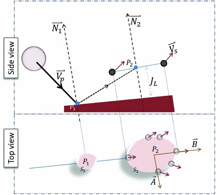
Figure 4. Splashing secondary droplets.
The operators ‖ used in Equations (19a)–(19f) are used to mean compute unit vectors from the vector within. The velocity magnitude for the unit vector
 $\overrightarrow{V}_s$
is from the experimental correlations. Equation (19f) is the parametric equation of a ring on a sphere of radius r (typically the crater radius). This equation describes the coordinates of a splashing droplets number i of a total of N
s
splashing droplets, and j = <1, 2, 3 > is the j
th component of the Cartesian coordinate. The number of droplets are spread by angle θ
i
about 0 to 2π.
$\overrightarrow{V}_s$
is from the experimental correlations. Equation (19f) is the parametric equation of a ring on a sphere of radius r (typically the crater radius). This equation describes the coordinates of a splashing droplets number i of a total of N
s
splashing droplets, and j = <1, 2, 3 > is the j
th component of the Cartesian coordinate. The number of droplets are spread by angle θ
i
about 0 to 2π.
In the review by Yarin(Reference Yarin5), a splash criteria is if approaching droplet velocity
 $U=18\left\lbrace \sigma /\rho _l \right\rbrace ^{\frac{1}{4}} \upsilon ^{\frac{1}{8}}f^{\frac{3}{8}} < U_{o}$
. It is assumed that the droplet is approaching the interface with a velocity, U
0. The kinematic viscosity is μ and the surface tension is σ. In the work of Samenfink et al(Reference Samenfink, Elsaßer and Wittig33), the splash criteria for film thickness in the range 0.5 < h* < 1.8 is when
$U=18\left\lbrace \sigma /\rho _l \right\rbrace ^{\frac{1}{4}} \upsilon ^{\frac{1}{8}}f^{\frac{3}{8}} < U_{o}$
. It is assumed that the droplet is approaching the interface with a velocity, U
0. The kinematic viscosity is μ and the surface tension is σ. In the work of Samenfink et al(Reference Samenfink, Elsaßer and Wittig33), the splash criteria for film thickness in the range 0.5 < h* < 1.8 is when
 $\frac{1}{24}Re \times La^{-0.4189}>1$
. Splash criteria for thin film impact proposed in Cossali et al(Reference Cossali, Coghe and Marengo10) is that We · Oh
−0.4 < K, where K = 2,100 + 5,880 · (h*)1.44. The number of secondary droplets created by a splash, for example, in Okawa et al(Reference Okawa, Shiraishi and Mori28), is N
s
= 7.84 · 10−6 · K
1.8(h*)−0.3. In crown splashing, the crown disintegrates into cusps and eventually into droplets. Rieber and Frohn(Reference Rieber and Frohn15) correlated the number of cusps from crown splashing as a function of non-dimensional time in the form A(T*)−B
, where A and B are constants depending on the case investigated. Other important correlations or parameters such as the velocity of exit of the droplets or the mass ejected exist in the literature(Reference Peduto, Koch, Morvan, Dullenkopf and Bauer16,Reference Mundo, Sommerfeld and Tropea26-Reference Okawa, Shiraishi and Mori28,Reference Bai and Gosman34,Reference Mehdizadeh, Navid and Mostaghimi35) . In this work, a simple presentation is used. The number of droplets are evenly distributed on the parametric curve. In the implementation of the splash model, it is important to take off the mass of the children droplets from the impacting droplets before the spread of the source term. The mass of the children droplets can simply be determined from their number and mean diameters. It is worth noting that codes developed can be enhanced in the future as new and more complete splashing model correlations become available.
$\frac{1}{24}Re \times La^{-0.4189}>1$
. Splash criteria for thin film impact proposed in Cossali et al(Reference Cossali, Coghe and Marengo10) is that We · Oh
−0.4 < K, where K = 2,100 + 5,880 · (h*)1.44. The number of secondary droplets created by a splash, for example, in Okawa et al(Reference Okawa, Shiraishi and Mori28), is N
s
= 7.84 · 10−6 · K
1.8(h*)−0.3. In crown splashing, the crown disintegrates into cusps and eventually into droplets. Rieber and Frohn(Reference Rieber and Frohn15) correlated the number of cusps from crown splashing as a function of non-dimensional time in the form A(T*)−B
, where A and B are constants depending on the case investigated. Other important correlations or parameters such as the velocity of exit of the droplets or the mass ejected exist in the literature(Reference Peduto, Koch, Morvan, Dullenkopf and Bauer16,Reference Mundo, Sommerfeld and Tropea26-Reference Okawa, Shiraishi and Mori28,Reference Bai and Gosman34,Reference Mehdizadeh, Navid and Mostaghimi35) . In this work, a simple presentation is used. The number of droplets are evenly distributed on the parametric curve. In the implementation of the splash model, it is important to take off the mass of the children droplets from the impacting droplets before the spread of the source term. The mass of the children droplets can simply be determined from their number and mean diameters. It is worth noting that codes developed can be enhanced in the future as new and more complete splashing model correlations become available.
2.4 Test cases, boundary conditions and simulation set-ups
There are three categories of simulations used in this work to showcase and evaluate the proposed model. These are for progressively checking (i) adequate mass conservation, (ii) momentum transfer and (iii) demonstrating splash formation using the proposed approach. Simple box type geometries with wall boundaries on all sides were used in the simulations. The dimensions of the boxes (H x × H y × H z ) are in multiples of the droplets’ diameters.
2.4.1 Mass conservation set-up
In this basic set-up, a single DPM droplet is injected at the centre of an empty box. The diameter, D p , of the droplet is 1,000 μm. The box is a cube with a width 15 × D p . In this test, four different mesh resolution set-ups are used. The meshes resolve the droplet by a spacing S*( = D p /h) in the zones indicated on Fig. 5 with the mesh becoming coarser away from the droplet as shown, where h is the grid spacing in the droplet zone. The S* cases tested are, respectively, 50, 25, 10 and 5.

Figure 5. Mesh used for single droplet DPM-CLSVoF test case.
The next basic test is for a train of DPM droplets injected into a box, as schematically shown in Fig. 6(a). The flow rate is specified for the Lagrangian droplet stream and expected to fill the box to a height, h. Particles with a density of 1,000 kg/m3 are injected into an initially dry box with a volume of 12 × 12 × 20 mm3. The mesh set-up is such that it is refined close to where the film is expected, Fig. 6(b).
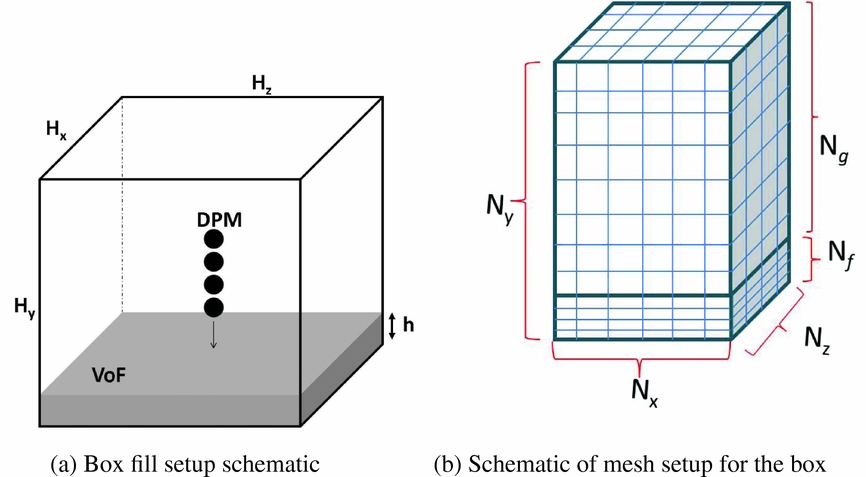
Figure 6. DPM-CLSVoF: Simple box fill set-up.
The number of nodes (N x , N y , N z ) used for mesh dependence studies are shown in Table 1. From Fig. 6(b), N f represents the number of nodes in the region where the film is expected. The target fill level is 1.2 mm for all the cases described in Table 2. The mass of the liquid expected is 172.8 mg in 1 s. The droplets are spaced every 5 × D p . In this simulation, the VoF timestep, ΔT, is 1 μs to limit the Courant number to less than 1. The convergence criteria set for all the equations are for a reduction of the residuals of four orders of magnitude at least for each equation. The final mass value and its stabilisation are another target.
Table 1 Box mesh dependence case set-up

Table 2 Box case set-up

aThe mass flow rate specified in ANSYS-Fluent GUI. This is the ratio of the mass of the droplet to the VoF timestep.
The third is a simple extension of the previous case to test capability for multiple droplets in a domain. In this case, batches of droplets with equal diameters of 260 μm are released into a box already partially filled with water. This physically represents a box being filled from a spray. Figure 7 shows the schematic of the box. H 0 is the initial level of the film before injection starts. The filling is done by the DPM droplets within the simulation duration and fill rate such that at the end of the simulation there should be liquid in the VoF representation up to a level of 2 × H 0 by the set-up in Table 3.

Figure 7. DPM-CLSVoF: Schematic of a train of multiple droplets.
Table 3 Train of multiple droplets case set-up

2.4.2 Demonstrating splash formation
The impact of a droplet at a high momentum may create a good number of smaller droplets. In practical applications of droplet to film impact, the secondary droplets are equally important to account for; the film and deformation caused by the impacting droplet can also play an important role. To demonstrate splashing from a VoF film and the formation of child DPM droplets, a parent DPM droplet is injected above a VoF film. The set-up follows that in the simulation work by Rieber and Frohn(Reference Rieber and Frohn15). The impact Weber number is 598, the Ohnesorge number, Oh, is 0.0014 and the film thickness, h*, is 0.116.
There are no complete sets of correlations that can completely predict all the parameters of any droplet splash scenario. The principles of operations of the model, developed here, are shown by taking several correlations from different sources in an attempt to capture the splashing droplets as much as possible. The number of DPM droplets generated(Reference Rieber and Frohn15) is estimated at T* = 0.1 using the correlation N s = 23.37(T*)−0.036 for this case. The mean diameters of the splashing DPM droplets are estimated from the mass of splashed droplets. Equation (20a) gives the experimental correlation(Reference Okawa, Shiraishi and Mori28) for the mass fraction splashed, E m , relative to the primary droplet. By the definition of mass fraction, Equation (20c), and mass balance, Equation (20e), the diameters of the secondary droplets, D s can be easily obtained. The magnitude of the velocity of the splashing droplets, Equation (19b), at the instance of creation is 52% of the impact velocity based on the observations(Reference Peduto, Koch, Morvan, Dullenkopf and Bauer16,Reference Okawa, Shiraishi and Mori28) that over 80% of the splashing droplets have this speed. In this test, there are 25 splashing droplets with an average diameter 15.18% of the primary droplet.
 $$\begin{eqnarray}
E_m = 0.00156e^{0.000486K}
\end{eqnarray}$$
$$\begin{eqnarray}
E_m = 0.00156e^{0.000486K}
\end{eqnarray}$$
 $$\begin{eqnarray}
K = We \cdot Oh^{-2/5}
\end{eqnarray}$$
$$\begin{eqnarray}
K = We \cdot Oh^{-2/5}
\end{eqnarray}$$
 $$\begin{eqnarray}
E_m =\frac{M_s}{M_p}
\end{eqnarray}$$
$$\begin{eqnarray}
E_m =\frac{M_s}{M_p}
\end{eqnarray}$$
 $$\begin{eqnarray}
M_p =\frac{\pi }{6} \rho _l D_p^3
\end{eqnarray}$$
$$\begin{eqnarray}
M_p =\frac{\pi }{6} \rho _l D_p^3
\end{eqnarray}$$
 $$\begin{eqnarray}
D_p^3 E_m =N_s D_s^3
\end{eqnarray}$$
$$\begin{eqnarray}
D_p^3 E_m =N_s D_s^3
\end{eqnarray}$$
2.4.3 Momentum transfer set-up
The crater evolution that results from the impact of a droplet on a film can be thought of as caused by the transfer of momentum from the droplet. Normal impact with a droplet velocity of U 0(m/s) is simulated. The ratio of liquid to gas density is 997 in all the cases. Other parameters are given in Table 4.
Table 4 Crater dynamics set-up details

2.4.4 Solution method
The solution is done in ANSYS-Fluent using the developed User Defined Function (UDF). The second order accurate upwind discretisation is used for the spatial terms of the governing equations. The first order accurate explicit time integration is used for the temporal terms. The choice of timestep is restricted with the Courant-Friedrichs-Lewy (CFL) number such that CFL < 1. This makes simulation timestep in the order of 1 μs. The first few timesteps into the solution are solved as a single phase before the introduction of the DPM or the liquid phase. The DPM tracking is done transiently and the breakup models, coalescence and other schemes have been disabled to reduce complexity.
3.0 RESULTS
3.1 Mass transfer
In converting from DPM to VoF, a sphere is expected after the conversion. The zero LS iso-surfaces in Figs 8(a)–8(d) show the conversions to the VoF droplets for the four levels of refinements in the single droplet test. The mesh refinement level relative to the droplet is described as the ratio of droplet-size to the grid-size (S* = D p /h). This shows a ‘loss in morphology’ is a result of the inability to resolve the droplet to a mesh by a coarser mesh, typical of the CLSVoF method. The finer the mesh, the better the resolution of the droplet free surface; it is, however, worth remembering that the number of cells required to resolve the droplet is actually (S*)3. The ‘mass loss’ to poor mesh resolution can be estimated from 100(1 − (R/R e )3), where R is the radius of the iso-surface and R e is the expected radius of the resulting VoF droplet.

Figure 8. Single DPM droplet turns VoF.
A resolution, S*, higher than 10 yields a mass conservation of over 99.6% in this single droplet test. From this simple test, a rule of thumb can be prescribed for mesh spacing in the wall regions to be of the order S* > 10, i.e. the mesh spacing to be a tenth of the mean droplet sizes, so that the first sets of DPM droplets landing on a dry wall can be resolved.
For the droplet train test, the volume of water in the geometry after the it settles down is compared with the expected volume of water (17.3 × 10⁻⁶ m3) in the box after 1 sec. The results for Meshes MSH 1, MSH 2 and MSH 3 given in Table 1 are off by 8.5%, 1.6% and 1.49%, respectively. The film grew from no-film at all to thicknesses, H* f , 1.5, 2.4 and 8.0 in the three cases. The final error is an accumulation from the inability to resolve the first sets of landing droplets but gets better as the film develops as shown in the next test. The qualitative film formation is shown in Fig. 9 for the 800 μm droplet filling the box to the marked level. The starting volume is 86.260 × 10⁻⁹m3 and the expected final volume is 172.520 × 10⁻⁹m3; the final volume computed using the finer mesh is 172.544 × 10⁻⁹m3, representing 0.013% difference; the coarser mesh with 25 nodes in the film gave a difference of 0.025%.

Figure 9. DPM-CLSVoF: Simple box fill results, 800 μm diameter droplet.
Figure 10 shows the transient film formation. The two red marks show the level to fill from and to fill to. This qualitatively shows the mass conversion; with only Fig. 10(c) showing the droplets forming the film.

Figure 10. DPM-CLSVoF: Simple multiple droplet box fill results.
3.2 Momentum transfer
The crater dynamics experiments for a normal impact of a single droplet on a known film thickness are presented in Fig. 11. The film thicknesses fall into thin (h* < 1) and thick (h* > 1) categories, with only the thin film case in the splashing category. The thin film results (h* = 0.116), are from the detailed simulations work of Rieber and Frohn(Reference Rieber and Frohn15), and the thick film experimental data of Cossali et al(Reference Cossali, Marengo, Coghe and Zhdanov11), as used in Peduto et al(Reference Peduto, Koch, Morvan, Dullenkopf and Bauer16). The crown diameter, is taken as an internal diameter of the crater, which is estimated on a fixed plane coinciding with the original film surface and the impact point. A generalisation of the crown rim evolution, as suggested by Cossali et al(Reference Cossali, Marengo, Coghe and Zhdanov11), is given in Equation (21). The constant C as proposed in Yarin and Weiss(Reference Yarin and Weiss29) is such that it is dependent on the initial film thickness, with C = (2/3h*)0.25 and n a square root form. X is the crater width and the droplet diameter at impact is D p . T*( = tU o /D p ) is the non-dimensional time and T* o is a time shifting constant.
 $$\begin{equation}
D^* = \frac{X}{D_p} = C \left( T^* - T^{*}_{o} \right)^n
\end{equation}$$
$$\begin{equation}
D^* = \frac{X}{D_p} = C \left( T^* - T^{*}_{o} \right)^n
\end{equation}$$

Figure 11. Crater evolution.
The experimental points are not connected with curves. The correlations, from Yarin and Weiss(Reference Yarin and Weiss29) and Equation (21), are given with the dashed lines. The solid lines are results from the proposed DPM-CLSVoF simulations. It can be seen that the patterns almost exhibit a square-root curve-fit form. It is worth noting that neither the published correlations nor the DPM-CLSVoF model exactly match the experimental data points for all conditions, but follow the similar patterns. It can be seen that the thin film crater growth rate is higher than those of the thick films. The mean deviations of the simulated D* from the corresponding reference data points are as 4.3%, 15.0% and 8.1%, respectively, for the relative thickness values of 0.116, 1 and 2.
3.3 Splashing and creation of child droplets
Figure 12 shows a demonstration of a normal droplet impact as done in the detailed simulation of Rieber and Frohn(Reference Rieber and Frohn15). The droplet impact Weber number is 598 on the film with a thickness, h*, of 0.116. The DPM-CLSVoF model is computed with about 0.5 million computational cells. The DPM-CLSVoF technique is clearly unable to resolve the splashing droplets as resolved by Rieber and Frohn(Reference Rieber and Frohn15) who used about 32.8 million computational cells. The DPM-CLSVoF technique, with that small number of cells, is not able to capture the full cusp and filament disintegration to droplets. Experimental correlations are used to predict the number and diameters of droplets in the splash. The otherwise ‘lost’ droplets are created at location A 1 for continued tracking. The droplets have been shown in a time-frozen frame to give an impression of the relative locations. The primary droplet impacts at A 0 and the splashing crown starts at A 1. The crown and the secondary droplets’ positions grow radially outwards. The film cross section is also shown, after source term exchanges.

Figure 12. DPM-CLSVoF: Normal splashing evolution -frozen in timesteps.
4.0 DISCUSSIONS
This work provides an insight into handling droplet splash from a film as a result of a primary droplet impact. The key insight provided is that an extremely fine mesh may not be required to handle small droplets that are usually encountered in real engine droplet to film applications. There are a number of limitations to this work even though it is promising for applications requiring higher mesh resolution. It is currently limited to spherical and non-deforming droplets. Droplet breakup models and coalescence models are not included. Large droplets sizes requiring spreading source terms over a wide zone may not produce stable results at impact. Unstable results are, as expected, observed when the magnitudes of the source terms are considerably larger than the magnitude of the components of terms in the Navier-Stokes equations. The timestep required for solution stability is of order of 1 micro-second or lower. The DPM-CLSVoF splash simulation presented here took less than 12 hours; a fully resolved splash on the same computer will take a couple of weeks to perform. The technique offers a cheap approximation to fully resolving the flow as Eulerian VoF and can be suited to complex geometries.
5.0 SUMMARY
There has been keen interest shown by researchers on droplets to film interaction because of its wide application. Post impact outcomes of the primary droplet on a surface include, but are not limited to, splashing, bouncing and sticking to the surface. The formation of film from droplet impact is useful, for example, in spray-film cooling. It is possible to model the detailed droplet film dynamics by fully resolving the flow with available CFD techniques. Many of these techniques, however, are computationally expensive because of the fine mesh requirements, thus, are not practical for complex geometries. In this paper, we attempted to reduce the complexity involved in droplet film dynamics by assuming that the droplets can be taken to be spherical particles that can be tracked using Lagrangian technique while the liquid film and the gas phases can be taken as Eulerian using the VoF technique. Although the coupling of Lagrangian particles with Eulerian phase is a known technique, it has not been done before as it is done here. The droplets tracking takes note of the current position and the source terms are distributed to the cells. The secondary droplets are modelled from existing correlations instead of resolving them. This creates the possibility to continue to track the secondary droplets from the film with the Lagrangian technique.
The developed model was tested using simple validations for mass and momentum transfer. Several basic tests were done for mass conservation check for the Lagrangian droplets turning to Eulerian VoF film and the accuracy ranged around 0.01% and 1.5% depending on how the film region is resolved. When a droplet impacts on a film, the consequence of momentum transfer is the crater evolution that follows it. This indirect check for momentum conservation is impressive when compared with published crater evolution results. The crater evolution simulations compare well with published correlations. For good results, the aim should be that the region where the film is most expected in the domain should be refined sufficiently to capture the film. It is not possible to be able to show detailed physics with this technique, but the solution relies on correlations to predict the impact outcome.


