


Introduction
Many paleoclimate records provide evidence of centennial and millennial (102–103 yr) hydroclimatic fluctuations and shifts during the Holocene, but the major patterns of variation at these time scales remain uncertain (Mayewski et al., Reference Mayewski, Rohling, Stager, Karlen, Maasch, Meeker and Meyerson2004; Wanner et al., Reference Wanner, Solomina, Grosjean, Ritz and Jetel2011; Roland et al., Reference Roland, Caseldine, Charman, Turney and Amesbury2014). Differences among archives and regions have been difficult to assess without systematic replication of the paleoclimatic signals, which, like modern droughts, can have a high degree of spatial heterogeneity. In the northeastern United States (U.S.), however, closely spaced paleohydrologic records present a useful opportunity to evaluate how millennial-to-centennial variability modified long-term regional moisture trends (Webb et al., Reference Webb, Anderson and Webb1993; Willard et al., Reference Willard, Bernhardt, Korejwo and Meyers2005; Li et al., Reference Li, Yu and Kodama2007; Newby et al., Reference Newby, Shuman, Donnelly and MacDonald2011; Marsicek et al., Reference Marsicek, Shuman, Brewer, Foster and Oswald2013). Work in this region can specifically evaluate climate dynamics associated with the North Atlantic (deMenocal et al., Reference deMenocal, Ortiz, Guilderson and Sarnthein2000; Oppo et al., Reference Oppo, McManus and Cullen2003; Thornalley et al., Reference Thornalley, Elderfield and McCave2009; Seager et al., Reference Seager, Pederson, Kushnir, Nakamura and Jurburg2012), while also documenting the long-term context for recent increases in effective moisture in the northeast U.S. (Pederson et al., Reference Pederson, Bell, Cook, Lall, Devineni, Seager, Eggleston and Vranes2013).
In the northeast U.S., the near-shore sediment stratigraphies of small lakes and ponds have indicated past water-level changes and have been used to quantify the timing and magnitude of hydroclimatic changes (e.g., Hubeny et al., Reference Hubeny, McCarthy, Lewis, Drljepan, Morissette, King, Cantwell, Hudson and Crispo2015). A series of studies using geophysical surveys, multiple sediment cores from each lake, and dozens of radiocarbon analyses spanning at least the last 6 cal ka BP have reconstructed repeated and synchronous precipitation minus evaporation (P-E) fluctuations of multi-century duration (Li et al., Reference Li, Yu and Kodama2007; Newby et al., Reference Newby, Shuman, Donnelly, Karnauskas and Marsicek2014). Additional evidence of multi-century variability derives from detailed stable isotopic records, which further demonstrate fluctuations of 330–500 yr (Zhao et al., Reference Zhao, Yu, Ito and Zhao2010). Multi-century water-level changes correlate across lakes (Newby et al., Reference Newby, Shuman, Donnelly, Karnauskas and Marsicek2014), with pollen-inferred precipitation reconstructions (Marsicek et al., Reference Marsicek, Shuman, Brewer, Foster and Oswald2013), and with both alkenone- and pollen-inferred temperature variability (Shuman and Marsicek, Reference Shuman and Marsicek2016).
The records indicate that a sequence of alternating warm-dry and cool-wet phases were superimposed upon a long-term increase in P-E of>400 mm since 9–8 ka (Webb et al., Reference Webb, Anderson and Webb1993; Shuman and Marsicek, Reference Shuman and Marsicek2016). Warm dry phases date to 4.9–4.6, 4.2–3.9, 2.9–2.1, and 1.3–1.2 ka from the inland Berkshire highlands to coastal Cape Cod about 200 km east (Newby et al., Reference Newby, Shuman, Donnelly, Karnauskas and Marsicek2014). These fluctuations may include the regional expression of variations discussed globally such as the 4.2- and 2.7-ka “events” (van Geel et al., Reference van Geel, Heusser, Renssen and Schuurmans2000; Booth et al., Reference Booth, Jackson, Forman, Kutzbach, Bettis, Kreig and Wright2005), but also place these events together as part of a potential series of genetically similar variations (Saltzman, Reference Saltzman1982; Renssen et al., Reference Renssen, Goosse and Muscheler2006; Jongma et al., Reference Jongma, Prange, Renssen and Schulz2007). However, a distinctive contrast between inland drought and a wet coast from 5.7–4.9 ka indicates that more than one dynamic was probably involved in the sequence of changes (Newby et al., Reference Newby, Shuman, Donnelly, Karnauskas and Marsicek2014). Changes from 5.7–4.9 ka may relate to a period with unusual North Atlantic circulation patterns and extensive climate anomalies across mid-latitude North America (Oppo et al., Reference Oppo, McManus and Cullen2003; Shuman and Marsicek, Reference Shuman and Marsicek2016), but could also be a function of lake-specific variability because the changes were only recorded at a single inland lake (Newby et al., Reference Newby, Shuman, Donnelly, Karnauskas and Marsicek2014).
To test whether multi-century variability detected in the northeast U.S., and the inland-coastal contrast there at 5.7–4.9 ka, represents a set of synoptic-scale variations or heterogeneous, sub-regional changes, we studied the water-level histories of two lakes in the northern Susquehanna River (Chesapeake Bay) watershed. The work extends a network of comparable, quantitative water-level reconstructions inland at the same latitude, which can connect the evidence of multi-century drought phases in Massachusetts (Newby et al., Reference Newby, Shuman, Donnelly and MacDonald2011, Reference Newby, Shuman, Donnelly, Karnauskas and Marsicek2014) with evidence of multi-century climate variability from New Jersey (Li et al., Reference Li, Yu and Kodama2007; Zhao et al., Reference Zhao, Yu, Ito and Zhao2010), Chesapeake Bay (Willard et al., Reference Willard, Bernhardt, Korejwo and Meyers2005), and lakes and bogs to the west from Ohio to Wisconsin (Baker et al., Reference Baker, Maher, Chumbley and Van Zant1992; Nelson et al., Reference Nelson, Hu, Grimm, Curry and Slate2006; Booth et al., Reference Booth, Brewer, Blaauw, Minckley and Jackson2012; Wang et al., Reference Wang, Gill, Marsicek, Dierking, Shuman and Williams2016).
Approach
We present evidence of lake level changes derived from ground-penetrating radar (GPR) profiles and closely dated lake sediment cores from two lakes, Blanding Lake (41.79°N, 75.68°W, 454 m elevation, 4.8 ha) and Handsome Pond (41.62°N, 75.68°W, 406 m elevation, 6.1 ha), in Susquehanna and Lackawanna Counties in northeastern Pennsylvania, respectively (Fig. 1). Both lakes lie within the glaciated, northeastern portion of the Allegany Plateau. They formed within the sandy Orlean Till above the Devonian Catskill Formation, comprised largely of red, fluvial sandstones (Berg et al., Reference Berg, Edmunds, Geyer, Glover, Hoskins, MacLachlan, Root, Sevon and Socolow1980; Sevon and Braun, Reference Sevon and Braun1997). They occupy small, well-defined watersheds and are drained by small streams. In the 45-ha watershed of Blanding Lake, elevations rise >50 m within 500 m of the lake, and they rise >35 m within 250 m of Handsome Pond, which has a 35-ha watershed. Today, a mix of deciduous forests, open fields, and rural housing cover the watersheds; a dense development of lake cabins rings Handsome Pond, but the shore of Blanding Lake is largely undeveloped.
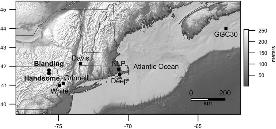
Figure 1 Map of the topography of the northeast United States, adjacent Canada, and the Atlantic Ocean showing the locations of our study sites (circles): Blanding Lake, Susquehanna County, Pennsylvania, and Handsome Pond, Lackawanna County, Pennsylvania. Other sites mentioned for comparison are shown as black squares. NLP, New Long Pond, Massachusetts.
To reconstruct the hydrologic history of each lake, we use a decision tree approach, implemented in R (R Core Development Team, 2009), to systematically evaluate and correlate data from multiple sediment cores (Pribyl and Shuman Reference Pribyl and Shuman2014). The approach constrains the elevation of shoreline sediments over time based on recognition of two major sedimentary facies: (1) a near-shore (littoral) zone with sandy, inorganic sediments that accumulate slowly (<20 cm/ka) due to erosion and degradation in warm, wind-mixed shallow (<1 m) waters; and (2) an offshore (profundal) zone of organic muds that typically accumulate at ~70 cm/ka across the range of depths (usually >1 m) where sediments fall out of suspension (Rowan et al., Reference Rowan, Kalff and Rasmussen1992; Shuman, Reference Shuman2003; Goring et al., Reference Goring, Williams, Blois, Jackson, Paciorek, Booth, Marlon, Blaauw and Christen2012; Shuman et al., Reference Shuman, Pribyl and Buettner2015). We infer intervals of low water from times when littoral sands extended to deeper positions within the lake basins than found today.
Individual cores can have idiosyncratic stratigraphies determined by bathymetry, local sediment supply, specific accumulation histories, and other factors, but multiple cores can be used together with GPR profiles to isolate the common stratigraphic signals created by changes in lake elevation. By quantitatively tracking the elevation of the littoral-profundal (sand-mud) boundary or “sediment limit” (Digerfeldt, Reference Digerfeldt1986), we can create lake-level time series, which are statistically comparable among lakes (Newby et al., Reference Newby, Shuman, Donnelly, Karnauskas and Marsicek2014; Pribyl and Shuman, Reference Pribyl and Shuman2014). GPR profiles ensure that key features represent basin-wide stratigraphic changes consistent with water level fluctuations rather than localized slumps or flood deposits (Pribyl and Shuman, Reference Pribyl and Shuman2014) and were collected at Handsome and Blanding lakes using a GSSI SIR-3000 GPR with a 400 MHz antenna floated in a small inflatable raft in June 2015. After quantifying the magnitude of the water-level changes at Blanding Lake, we also use a simple mass-balance approach applied at multiple other lakes to estimate changes in P-E from the changes in lake volume (Shuman et al., Reference Shuman, Pribyl, Minckley and Shinker2010; Marsicek et al., Reference Marsicek, Shuman, Brewer, Foster and Oswald2013; Pribyl and Shuman, Reference Pribyl and Shuman2014). Like previous work, we made no assumptions or adjustments about the effects of sediment compaction on the elevations of stratigraphic features.
In combination with the GPR data, multiple cores were collected in water depths of <1.5 m and <50 m from shore at the two lakes. The cores were collected in June 2015 with a 7 cm diameter Wright piston corer using 1 m polycarbonate barrels to obtain successive contiguous core sections representing the entire lacustrine sediment sequence at each location. The cores were capped and returned to the University of Wyoming before opening and sampling, and foam was inserted in barrel tops to stabilize the uppermost, flocculent sediment during transport and storage. We used loss-on-ignition (LOI) analyses (Dean, Reference Dean1974; Shuman, Reference Shuman2003) of contiguous 1 cm3 sub-samples to quantify the stratigraphic changes in each core because alternating layers of sand (low LOI) and mud (high LOI) were visually apparent upon collection. When the Holocene sediment samples were combusted at 550°C for 2 hrs, LOI <20% indicated the presence of littoral sands associated with a low weight percent of organic mater (Shuman, Reference Shuman2003; Shuman et al., Reference Shuman, Pribyl and Buettner2015).
Net sediment accumulation rates between calibrated radiocarbon ages further confirm the interpretation of sand layers within the cores because littoral sands have low accumulation rates relative to profundal muds (Shuman et al., Reference Shuman, Pribyl and Buettner2015), and especially compared to rapidly accumulated slumps or flood deposits (e.g., Munoz et al., Reference Munoz, Gruley, Massie, Fike, Schroeder and Williams2015). All radiocarbon ages, based on analyses of sedimentary charcoal analyzed at the Keck Carbon Cycle AMS Facility at the University of California Irvine, were calibrated using Intcal13 in Bchron (Haslett and Parnell, Reference Haslett and Parnell2008; Reimer et al., Reference Reimer, Bard, Bayliss, Beck, Blackwell, Bronk Ramsey and Buck2013).
We compare our lake-level reconstructions with other paleoclimate records using generalized least squares (gls) regression in R using the function “gls” (Pinheiro and Bates, Reference Pinheiro and Bates2000). The mixed effects approach enables the errors to be correlated in the models to account for temporal autocorrelation. To do so, we assume a first-order autoregressive moving average (ARMA) relationship among model residuals. To further assess correlations among multi-century changes rather than driven by long trends, we also compared records after fitting and removing models of Northern Hemisphere June insolation trends (Berger and Loutre, Reference Berger and Loutre1991). To account for uneven spacing of samples in time in the different cores, both the lake-level reconstruction process and the gls models were applied after interpolating core data to 50-yr intervals based on the median age models. No further chronological adjustments were made.
RESULTS
Near-shore sediment stratigraphies
Bright reflectors in GPR profiles from Blanding Lake and Handsome Pond extend outward from shore and interrupt the near-shore sequences of the late Quaternary lake sediments (Fig. 2). The reflectors meet expectations for paleoshorelines associated with near-shore erosion during periods of low water (Pribyl and Shuman, Reference Pribyl and Shuman2014). They extend from multiple sides of the lake basins and truncate underlying units. Mud units that correlate with the bright near-shore reflectors (dark lenses extending from the end of the bright reflectors in Fig. 2) indicate periods when profundal muds were constrained to narrow, deep areas (as expected during periods of low water). They pinch out toward shore between the bright reflectors (e.g., between reflectors IIa and IIb in Fig. 2A).
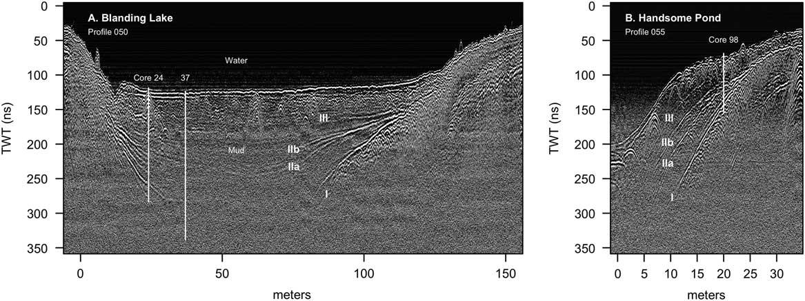
Figure 2 Ground-penetrating radar (GPR) profiles from (A) Blanding Lake and (B) Handsome Pond, Pennsylvania (Fig. 1). Vertical lines show the approximate positions of sediment cores (Fig. 3) and numerals I–III mark the distal edges of three major near-shore reflectors interpreted as paleoshoreline deposits. Vertical axis represents the data with respect to two-way travel time (TWT) of the radar signal; data were collected using a 400 Mhz antenna.
Based on the GPR profiles, two near-shore cores were obtained from 199 cm water depth at 37 and 24 m from the south shore of Blanding Lake and one from 98 cm water depth ~15 m from the northwest shore of Handsome Pond (Table 1 and Fig. 2). The Blanding Lake cores are labeled by distance from shore because they have the same water depth today. All depths in cores are given relative to the lake surface during coring (July 2015).
Table 1 Cores collected in June 2015.

Cores collected through the near-shore sequences of Holocene sediment contain alternating layers of organic-rich muds with high net sediment accumulation rates and inorganic, sand layers with low net sediment accumulation rates (Fig. 3). At Blanding Lake, intervals of sands are associated with 2–20% LOI (units I–III in Fig. 3A and B) and stand out visually, such as in core 24 at 299–309, 329–331, 337–343, and 347–352 cm depth, where LOI is <10% (Fig. 3B). At Handsome Pond, visual sands in core 98 also coincide with minima in LOI (<20%) at 164–184 and 191–193 cm depth (Fig. 3C); three distinct layers from 164–171, 174–176, and 181–183 cm compose the upper sand unit and contain wood fragments that raise LOI as high as 20%.
At both lakes, the sand units in the cores appear consistent with major near-shore reflectors in the radar stratigraphies (e.g., reflectors I–III in Fig. 2A). The most closely spaced sets of sand layers in the cores correlate with branches of the major radar reflectors, which indicate that the layers diverge, become thin, and terminate at different distances outward from shore (Fig. 2). For example, we correlate the branching of reflectors IIa and IIb at Blanding Lake (Fig. 2A) with the sequence of sand layers between 329–352 cm depth in core 24 (Fig. 3B). Not all of these sand layers appear to extend to core 37, but layer II at 347–352 cm in core 24 extends outward from shore to 436–457 cm in core 37 (gray bar, Fig. 3A and B). Similarly, at Handsome Pond, radar reflectors IIa and IIb converge at the location of core 98 (vertical line in Fig. 2B), which is consistent with the multiple, closely spaced sand layers that form the low-LOI (<20%) unit from 163–193 cm (Fig. 3C).

Figure 3 Stratigraphic data from cores collected from (A–B) Blanding Lake and (C) Handsome Pond, northeast Pennsylvania. Loss-on-ignition (LOI) data plotted on the left indicate the percent dry mass combusted at 550°C. Low values (e.g., gray bars) represent sand-rich intervals in cores collected in 199 (A–B) and 98 cm of water (C). Net sediment accumulation rates (in cm/ka) indicate that sandy, low LOI intervals represent reduced accumulation in shallow water; these data are shown on a log scale to the right for each core and were calculated between calibrated radiocarbon ages (Table 2; horizontal lines labeled with median age rounded to decade in cal yr before AD 1950). The elevations and ages of the cores from Blanding Lake (plotted in D) were used with the LOI data to constrain the position of the littoral zone through time. Core intervals were classified as littoral (orange symbols in D) based on bootstrapped classification schemes to produce an ensemble of reconstructions (gray lines in D). The median reconstruction (dark blue) and associated 95% range of elevational uncertainty (light blue band) are shown and used as an approximation of the lake elevation through time (Fig. 4). (For interpretations of the references to color in this figure legend, the reader is referred to the web version of this article.)
Table 2 Radiocarbon analyses.

a Ages not accepted; out of stratigraphic order
b Sample masses <1 mg C are listed.
In all three cores, low net sediment accumulation rates coincide with the low LOI (<20%) sand layers (Fig. 3A-C), which is consistent with modern littoral sediments (Shuman et al., Reference Shuman, Pribyl and Buettner2015) and thus an expansion of the littoral zone during episodes of low water. Accumulation rates as low as 2 cm/ka likely indicate depositional hiatuses and their constraining ages overlap in Blanding cores 37 and 24 and Handsome core 98, respectively, at (1) >6.2, >6.8, and >7.4 cal ka BP; (2) 5.5–4.4, 6.3–4.9, and 6.4–4.9 cal ka BP; and (3) 2.8–1.9, 3.3–2.0, and 3.0–0.5 cal ka BP (Fig. 3, gray bars). Low LOI (<10%) and low accumulation rates (<20 cm/ka) also overlap in time in the two shallowest cores, Blanding 24 and Handsome 98, at 5.1–3.8 and 4.9–3.4 cal ka BP, respectively (Fig. 3B and C), when accumulation rates in the deepest core, Blanding 37, remained low (until 3.5 ka, Fig. 3A). Maxima in accumulation rates of >50 cm/ka correspond to high LOI muds, like those typically found in >1 m of water today (Shuman et al., Reference Shuman, Pribyl and Buettner2015), and are bracketed by calibrated radiocarbon ages in Blanding 24 at 6.8–6.3, 3.8–3.3, and 2.0–1.0 cal ka BP (Fig. 3B) and Handsome 98 at 7.4–6.9, 3.4–3.0, and <0.5 cal ka BP (Fig. 3C).
To enable sand to accumulate in Blanding Lake core 37, the littoral zone must have been at least 3.0, 2.25, and 1.25 m lower than today at 12.1–6.2, 5.5–4.4, and 2.8–1.8 ka, respectively, given the directly measured elevations of the sand layers in the core (Fig. 3D). Additional water-level changes of ~50 cm could also explain the less extensive sand layers in Blanding core 24 between 4.9 and 3.8 ka (Fig. 3A and B). At Handsome Pond, the core does not include dated sediments older than 7.4 ka, which indicates that water levels were likely lower than the core location until the early Holocene. Subsequent fluctuations would have had to shift the littoral zone to more than 150–200 cm below the modern water surface to deposit the coalesced sand layers in core 98 (Fig. 3C).
Comparisons with other records
Since 7 ka, the cores from Blanding Lake contain sufficient detail to generate a quantitative lake-level reconstruction (Fig. 3D). The reconstruction represents a parsimonious interpretation of the changes in the two cores from Blanding Lake, and indicates that the lake rose progressively during the Holocene. The long-term rise is qualitatively consistent with the onset of sediment accumulation in Handsome Pond core only after ca. 7 ka and with the accumulation of high LOI (>40%) muds in all cores only after 3.3–1.8 ka (Fig. 3). The inferred changes would have affected each individual core in a unique way based on each core’s depth and accumulation history, and, as a result, no two cores have exactly the same stratigraphic sequence. Because Handsome Pond core 98 represents a shallower location than the other two cores, the stratigraphy represents a compressed sequence of changes with high-LOI muds accumulating during only the highest water phases.
The reconstruction indicates that units I–III represent multi-century drought phases, which punctuated the long-term rise (Fig. 3D). The elevations and common periods of overlap in the ages of sand layers from the different cores provide evidence that the level of Blanding Lake fell to minima relative to the long-term trend at 5.5–4.4, >3.8, and 2.8–2.0 cal ka BP. The most prominent intervening maximum dates to ca. 3.4 cal ka BP (Fig. 3D). Handsome Pond contains a compressed sequence of sand and mud layers that overlaps in time with these events (Fig. 3C), but more generally, the reconstructed changes correlate with the reconstructed histories of other lakes in the region (Fig. 4A).

Figure 4 Lake-level histories (blue lines in A) and sea-surface temperatures (SSTs in red on an inverted scale in A) indicate that integrated terrestrial-marine changes altered the coastal moisture gradient in multiple ways over 102–104 yrs (Sachs, Reference Sachs2007; Newby et al., Reference Newby, Shuman, Donnelly, Karnauskas and Marsicek2014). Scatter plots (B–E) show residual correlations among lakes and SSTs after removing the correlated long trends (dashed in A) and use the same x-axis ranges for coastal New Long Pond (B) and inland Blanding Lake (C–E with coefficients, r, listed). Generalized least squares models (lines) account for temporal autocorrelation and show the dominance of correlated multi-century changes, but small symbols represent periods from >4.5 ka when coastal and inland lakes were out of phase. Standard deviation (sd) units account for different lake sizes and depth ranges. Vertical bars in A represent coastal dry periods from Newby et al. (Reference Newby, Shuman, Donnelly, Karnauskas and Marsicek2014) with no significant age differences between Deep and New Long ponds. (For interpretations of the references to color in this figure legend, the reader is referred to the web version of this article.)
The changes at other lakes correlate with sea-surface temperature (SST) variations recorded in adjacent regions of the western North Atlantic (Fig. 4A and B). Long-term increases in the lake levels can be explained by seasonal insolation trends (dashed lines in Fig. 4A; Berger and Loutre, Reference Berger and Loutre1991), which in simulations reduced summer temperatures and evaporation since the mid-Holocene while also increasing the advection of sub-tropical moisture to the region (Webb et al., Reference Webb, Anderson and Webb1993, Reference Webb, Anderson, Webb and Bartlein1998; Harrison et al., Reference Harrison, Bartlein, Brewer, Prentice, Boyd, Hessler, Holmgren, Izumi and Willis2014). The correlations among lakes persist even after summer insolation trends have been fit and removed (Fig. 4B–E). Generalized least squares regressions (lines in Fig. 4C–E) indicate that the correlations with the detrended Blanding Lake reconstruction over the past 4.5 ka typically have positive slopes, indicative of significant correlations when they differ from zero (β=0.58±0.06, 0.18±0.07, and 0.78±0.06 for Davis, Deep, and New Long ponds, respectively).
From ca. 5.7–4.9 ka, however, Blanding Lake, like Davis Pond in western Massachusetts, fell when the two coastal lakes, New Long and Deep ponds in eastern Massachusetts, rose and SSTs declined (Fig. 4A, note inverted SST scale). Sand layer II at Blanding Lake and the associated minimum in accumulation rate dating from 5.5–4.4 cal ka BP in core 37 and 6.3–4.9 cal ka BP in core 24 (Fig. 3A and B) is similar in age to a low-water sand layer dating from 5.6–4.9 cal ka BP at Davis Pond (in core F, 10 m from shore; Newby et al., Reference Newby, Shuman, Donnelly and MacDonald2011). The two coastal lakes, however, do not have evidence of sand accumulation in near-shore cores until 4.9–4.6 ka (Newby et al., Reference Newby, Shuman, Donnelly, Karnauskas and Marsicek2014), and the slopes of generalized least squares regressions comparing Blanding and the coastal lakes before 4.5 ka were negative (β=−1.15±0.30 and −1.37±0.36 for the relationships between the detrended reconstructions of Blanding Lake and Deep and New Long ponds, respectively; small symbols in Fig. 4C and D). The onset of the coastal drought marks the beginning of in-phase changes based on continued accumulation of littoral sands in Blanding core 37 until an age of 4.4 cal ka BP (Fig. 3A) and a second discrete sand layer and accumulation rate minimum dating to 4.9–4.4 cal ka BP at Handsome Lake (represented as a LOI minimum in Fig. 3C).
The lakes reached their highest water-level phases during the last 2 ka (Fig. 4A), when Blanding Lake rose to a stable level associated with its current outlet (Fig. 3D). Sandy layers near the tops of cores 37 and 24 indicate some additional variations in water level (Fig. 3A and B), but the elevations of the sands did not fall substantially below the modern elevation of the littoral zone (Fig. 3D).
The Blanding Lake water level reconstruction also correlates with the oxygen isotope record from endogenic carbonates within Lake Grinnell, New Jersey (Fig. 5). High δ18O values at Lake Grinnell have been interpreted as evidence of regional warmth (Zhao et al., Reference Zhao, Yu, Ito and Zhao2010). The negative correlation with the Blanding Lake reconstruction (r=−0.76), thus, supports the negative correlation with Scotian Margin SSTs (Sachs, Reference Sachs2007; Fig. 4A and B). Cool periods (low δ18O) tended to be associated with high water, and warmth (high δ18O) with drought. The relationship could also represent possible evaporative influences on the δ18O record.
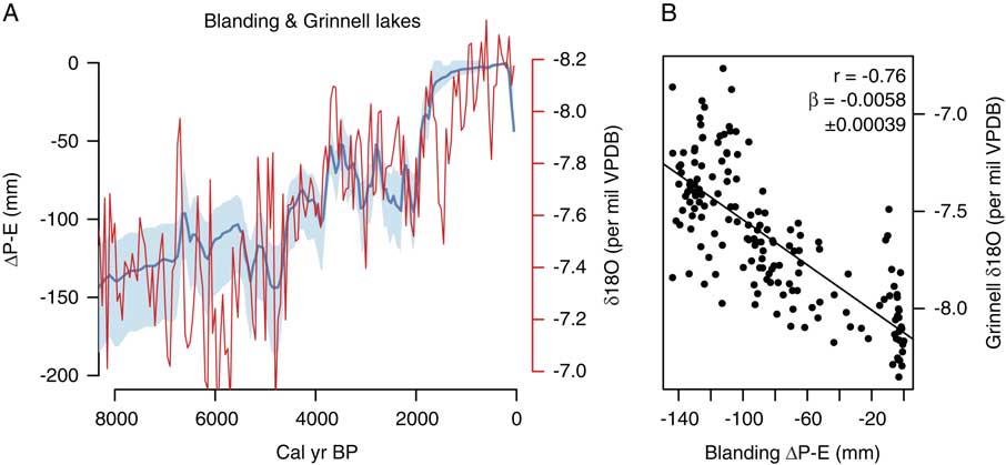
Figure 5 The change in the balance of precipitation minus evaporation (ΔP-E, blue in A) required to lower Blanding Lake after desiccation of its outlet stream correlates with the δ18O record (red with inverted scale in A) from Lake Grinnell, New Jersey, 120 km southeast (Zhao et al., Reference Zhao, Yu, Ito and Zhao2010). Line in B represents a generalized least squares model of the relationship with slope, β. No adjustments were made to either chronology in making this comparison. ΔP-E was calculated using the bootstrapped hydrologic budget approach of Pribyl and Shuman (Reference Pribyl and Shuman2014). (For interpretations of the references to color in this figure legend, the reader is referred to the web version of this article.)
The median age models for the two records indicate that synchrony cannot be ruled out for shifts in both records at ca. 4.7, 3.8, and 2.0 ka, but the δ18O also contains evidence of variability at higher frequencies than the fluctuations that produced units I-III at Blanding. For example, the period of low water from 5.5–4.7 ka coincides with high variability in the δ18O record rather than persistently high δ18O values, although the mean δ18O for the period is higher than any subsequent >200 yr window. The most pronounced difference exists from 6.3–5.5 ka (Fig. 5A), when organic silts below unit II (Fig. 3A and B) indicate high water, but δ18O reach a maximum (Fig. 5A). Although the δ18O provide added detail to the time series of events, specific P-E estimates can only be made from the lake-level record. The estimates indicate that the multi-century events represent changes of ~50 mm (Fig. 5).
Discussion
The water-level histories of Blanding Lake and Handsome Ponds clarify that the northeast U.S. has been much drier than today for most of the period since deglaciation and that repeated multi-century drought phases punctuated the long-term increase in effective moisture since 7–6 ka. The long-term trends have been attributed to the regional effects of the Laurentide Ice Sheet and orbital change on the advection of moisture into the region (Webb et al., Reference Webb, Anderson and Webb1993; Shuman et al., Reference Shuman, Bartlein, Logar, Newby and Webb2002), but the multi-century variability has not been as clearly diagnosed (Li et al., Reference Li, Yu and Kodama2007; Newby et al., Reference Newby, Shuman, Donnelly, Karnauskas and Marsicek2014). The correlation of our new records with water-level variations in coastal Massachusetts and with SSTs associated with the Labrador Current (Fig. 4) appear to confirm a regional hydrologic interconnection with the state of the North Atlantic (Li et al., Reference Li, Yu and Kodama2007). The correlated changes do not, however, clarify whether the ocean was the driver of the dynamics or another parallel aspect of the hierarchy of regional changes (Seager et al., Reference Seager, Pederson, Kushnir, Nakamura and Jurburg2012).
The formation of sand layers in the cores from the two lakes during low water dated at 12.1–7.4, 6.3–4.9, >3.7, and 2.8–2.0 cal ka BP closely parallels the history of Davis Pond 192 km east in the Berkshire Hills of western Massachusetts (Fig. 4; Newby et al., Reference Newby, Shuman, Donnelly and MacDonald2011, Reference Newby, Shuman, Donnelly, Karnauskas and Marsicek2014). The episodes of low water extended sands out from shore at least as far as Blanding Lake core 37, which was usually deep enough to accumulate organic-rich muds (Fig. 3A and D). High water episodes such as at ca. 3.3 cal ka BP and after 1.8 cal ka BP extended the muds at least as far toward shore as Blanding Lake core 24, which often accumulated low-LOI sands in the shallow littoral zone (Fig. 3B–D). The fluctuations may support the inference of droughts and low water phases from the expansion of littoral marls at White Lake, New Jersey at ca. 6.1, 4.4, and 3.0 ka (Li et al., Reference Li, Yu and Kodama2007). Lakes in the region also contain evidence of another drought phase at ca. 1.3 ka, although Blanding Lake appears to have been overflowing by this time and the associated sand layer (low LOI in Fig. 3A and B) is bracketed by a mix of out of order ages from 1.4–1.0 cal ka BP.
If the evidence of drought phases at 4.9–3.8 and 2.8–2.0 cal ka BP represents the regional expression of the 4.2- and 2.7-ka “events” (van Geel et al., Reference van Geel, Heusser, Renssen and Schuurmans2000; Booth et al., Reference Booth, Jackson, Forman, Kutzbach, Bettis, Kreig and Wright2005; Martin-Puertas et al., Reference Martin-Puertas, Matthes, Brauer, Muscheler, Hansen, Petrick, Aldahan, Possnert and van Geel2012; Roland et al., Reference Roland, Caseldine, Charman, Turney and Amesbury2014), then the two events may have had related causes or similar climate dynamics in the northeast U.S. In the first case, sand layers in the two shallowest cores (Blanding 24 and Handsome 98) date to 4.9–3.8 cal ka BP (Fig. 3B and C), and thus broadly overlap in time with hydrologic fluctuations identified elsewhere (Booth et al., Reference Booth, Jackson, Forman, Kutzbach, Bettis, Kreig and Wright2005). However, our quantified reconstruction for Blanding Lake indicates that water levels reached their maximum drawdown during the event at 4.0–3.7 cal ka BP (Fig. 3D) based on the interpolated ages of sandy low LOI intervals in the deepest core, Blanding 37 (Fig. 3A). A calibrated radiocarbon age reversal in Blanding core 24 at 5.1–3.8 ka limits our ability to refine the local chronology of the event (Fig. 3B). In the case of the changes at ca. 2.7 cal ka BP, the overlapping ages of the littoral sediment deposition in all of the cores overlaps directly with the event as defined elsewhere: 3.3–2.0 ka (Martin-Puertas et al., Reference Martin-Puertas, Matthes, Brauer, Muscheler, Hansen, Petrick, Aldahan, Possnert and van Geel2012).
Regionally, both fluctuations appear to be part of a series of repeated departures from the long-term hydrologic trends, which have consistent relationships to changes in the nearby ocean (Fig. 4A and B) and to multi-century temperature changes in Greenland (Newby et al., Reference Newby, Shuman, Donnelly, Karnauskas and Marsicek2014). The White Lake record has been correlated to the timing of ice-rafted debris events in the North Atlantic, which led to the interpretation that the events represent cold-dry phases (Li et al., Reference Li, Yu and Kodama2007), but the lake-level reconstructions in Fig. 4 consistently show a negative correlation to SST variations from the Scotian Margin since 4.5 ka (Fig. 4A) and to oxygen isotopic changes at Lake Grinnell (Fig. 5; Zhao et al., Reference Zhao, Yu, Ito and Zhao2010). The regional expression of these events may have been warm, dry departures from the long trends, which is consistent with pollen-inferred temperature and precipitation reconstructions of the same events in Massachusetts (Marsicek et al., Reference Marsicek, Shuman, Brewer, Foster and Oswald2013; Shuman and Marsicek, Reference Shuman and Marsicek2016).
The similarity of events over the past 8 ka at the coastal lakes (Fig. 4A and B) indicates that at least one type of recurring climate dynamic produced multi-century fluctuations near the western North Atlantic, but our results also show that a different chain of processes were involved in changes from ca. 5.5–4.4 ka. As the region cooled at 5.5 ka, coastal lakes rose but the western lakes declined (Fig. 4; Newby et al., Reference Newby, Shuman, Donnelly, Karnauskas and Marsicek2014). High variability in δ18O at Lake Grinnell could confirm that the other records provide a time-averaged record of sub-centennial variability, but could also represent an intermediate location fluctuating between positive (coastal) and negative (inland) responses. The differences between the Blanding and Grinnell records at ca. 6 ka (Fig. 5) are similar to the difference between Blanding and the coastal lakes like Deep Pond (Fig. 4). The anti-phased changes could have also emerged from a single abrupt shift in the long-term mean states at ca. 5.5 ka (Kirby et al., Reference Kirby, Mullins, Patterson and Burnett2002) when other abrupt changes took place in this region (e.g., a permanent shift in pine pollen percentages in cores from Chesapeake Bay, Willard et al., Reference Willard, Bernhardt, Korejwo and Meyers2005) and across the North Atlantic basin (McGee et al., Reference McGee, deMenocal, Winckler, Stuut and Bradtmiller2013).
Evidence of similarly timed drought phases exists as far west as Chatsworth Bog, Illinois, and Devils Lake, Wisconsin, where peaks in pollen from prairie forbs indicate an eastward expansion of prairie and where oxygen isotopes indicate aridity from ca. 5.5–4.9 ka (Baker et al., Reference Baker, Maher, Chumbley and Van Zant1992; Nelson et al., Reference Nelson, Hu, Grimm, Curry and Slate2006; Grimm et al., Reference Grimm, Maher and Nelson2009). Abrupt tree declines, shifts in lake sediment composition, and periods of bog desiccation in Indiana, Michigan, and Ohio may also represent responses to the same event (Booth et al., Reference Booth, Brewer, Blaauw, Minckley and Jackson2012; Wang et al., Reference Wang, Gill, Marsicek, Dierking, Shuman and Williams2016). More work is needed to understand the extent of this mid-Holocene arid phase, but it caused water levels to decline sufficiently to produce low LOI sand layers with the lowest net sediment accumulation rates of the past 7 ka at both Blanding Lake and Handsome Pond beginning between 6.3–5.5 ka and ending between 4.9–4.4 ka (Fig. 3).
Finally, the accumulation of high LOI muds in all of our cores since ca. 1.8 ka underscores the unusually cool, wet nature of the Common Era in this region. Given that sediment accumulation should have made the core locations shallower with time, the low sand content and high LOI of the upper meter of sediments provides strong evidence of a water level rise. Shallowing with time should have made it easier to deposit sand and winnow organic matter from the core sites, but the cores show the opposite pattern. The recent high water (Fig. 4) confirms that historical conditions do not represent the long-term mean state under which many ecological or geomorphic systems in this region developed during the Quaternary (Shuman et al., Reference Shuman, Newby, Huang and Webb2004; Brantley et al., Reference Brantley, Lebedeva, Balashov, Singha, Sullivan and Stinchcomb2016). Recent regional increases in effective moisture, therefore, probably also lack precedent within the Holocene (Seager et al., Reference Seager, Pederson, Kushnir, Nakamura and Jurburg2012; Pederson et al., Reference Pederson, Bell, Cook, Lall, Devineni, Seager, Eggleston and Vranes2013).
Declines in LOI in the top 20 cm of the cores may indicate that the highest water levels were achieved before 0.5 cal ka BP (Fig. 3). A water-level decline since then would be inconsistent with a multi-century increase in effective precipitation inferred from tree-ring records since AD 1500 (Pederson et al., Reference Pederson, Bell, Cook, Lall, Devineni, Seager, Eggleston and Vranes2013). However, several caveats apply. First, land clearance following European settlement would have facilitated erosion into the lakes at rates with few Holocene precedents and, although more sand was transported into the littoral zone, a decrease in the elevation of the shoreline during low water is not indicated by the elevations of these uppermost sands. Unlike older sand layers, the uppermost sands could have formed with little change in the elevation of the littoral zone (Fig. 3D). Likewise, net sediment accumulation rates did not consistently decline, as observed during other inferred low stands (e.g., Fig. 3C). Second, even if water levels fell from their late Holocene maxima, we cannot rule out the importance of erosion at the lake outlets, which have spillover points today <50 cm below the lake surface. Earlier levels were well below these thresholds, but the outlets may have expanded once they were breached by high water since ca. 1.8 cal ka BP.
Conclusions
Lake-level studies from northeastern Pennsylvania confirm that long-term hydrologic trends raised water tables by several meters in the northeast U.S. in response to ice sheet, insolation, and greenhouse forcing over the Holocene. Furthermore, millennial to centennial variations that interrupted these trends were correlated with changes in the North Atlantic and produced at least two different spatial patterns of drought in the region. The first pattern produced low water levels from Pennsylvania to coastal Massachusetts from ca. 4.9–3.8 and 2.8–2.0 ka when regional temperatures were high, but the second pattern increased water levels along the coast while lakes and wetlands in Pennsylvania, western Massachusetts, and portions of the Great Lakes region fell from 5.5–4.9 cal ka BP. Multiple cores within individual lakes (Fig. 3) and across multiple lakes replicate the stratigraphic signals (Fig. 4), but the synoptic extent and dynamics associated with these changes require further investigation as part of the full spectrum of hydroclimate variability. Similar datasets in additional areas could provide specific estimates of P-E and show the spatial patterns of change as a means to further diagnose multi-century hydroclimate variability.
ACKNOWLEDGMENTS
Funding for this project as provided by NSF ESPCoR (EPS-1208909) and Ecosystem Studies (DEB-1146297). We thank J. Yelton, R. Davis, N., J. Calder, and M. Serravezza for assistance with field and lab work, R. and N. Nesky and W. Smith III for access to the lakes, and two anonymous reviewers for useful comments on the manuscript.


