


1. Introduction
Curved pipes have a wide range of applications in the industry because of their enhanced mixing properties, high heat transfer coefficient and compact structure. Examples of application include, but are not limited to, heat exchangers, air-conditioning systems, chemical reactors and steam generators (see the reviews by Naphon & Wongwises (Reference Naphon and Wongwises2006) and Vashisth, Kumar & Nigam (Reference Vashisth, Kumar and Nigam2008)). One of the crucial questions in the study of turbulent flows in curved pipes is the accurate determination of the dependence of the flow rate and friction factor on the applied pressure difference between the two ends of the pipe, as well as their dependence on geometric parameters such as the pipe's curvature and torsion. The extensive usage of curved pipes in the industry has motivated many studies to characterize this dependence (Itō Reference Itō1959; Liu & Masliyah Reference Liu and Masliyah1993; Yamamoto, Yanase & Yoshida Reference Yamamoto, Yanase and Yoshida1994; Yamamoto et al. Reference Yamamoto, Akita, Ikeuchi and Kita1995; Cioncolini & Santini Reference Cioncolini and Santini2006). However, only a few of these studies consider the high-Reynolds-number limit, which is the objective of this paper.
The flow structure inside a curved pipe can vary substantially with Reynolds number and pipe geometry, which leads to a number of different regimes, each with its own distinct functional dependence of the flow rate and friction factor on these parameters. Therefore, unlike in the case of a straight pipe, quantifying this dependence becomes difficult even for the laminar flow. Indeed, at low Reynolds number, an imbalance between centrifugal force and cross-stream pressure leads to the onset of secondary counter-rotating vortices known as Dean's vortices, which were first experimentally observed by Eustice (Reference Eustice1910, Reference Eustice1911). Dean (Reference Dean1927, Reference Dean1928) confirmed this observation analytically in the low-curvature limit by computing the flow velocity as a perturbation of the well-known laminar Poiseuille flow solution. Dean (Reference Dean1928) showed that the effect of curvature is to decrease the flow rate and that this effect is of second order, i.e. quadratic in curvature. Several other studies were performed in the small-curvature limit to obtain a steady-state flow solution in a toroidal pipe; see for example McConalogue & Srivastava (Reference McConalogue and Srivastava1968), Van Dyke (Reference Van Dyke1978) and Dennis (Reference Dennis1980). For a comprehensive review of the topic, the reader is referred to Berger, Talbot & Yao (Reference Berger, Talbot and Yao1983). Germano (Reference Germano1982) further extended Dean's result to a helical pipe with small torsion, and Tuttle (Reference Tuttle1990) showed that small torsion leads to a second-order decrease in the flow rate. However, no analytical result exists for the steady flow in a pipe with a finite radius of curvature or torsion. Therefore, even in the laminar regime, one has to rely on empirical formulae to quantify the flow rate.
The transition to turbulence in curved pipes also differs substantially from the case of a straight pipe. Taylor (Reference Taylor1929) and White (Reference White1929) found that flow in a curved pipe is more stable than in a straight pipe. Notably, they saw that the critical Reynolds number for the transition is twice as large as in the straight pipe case. Inspired by this observation, Sreenivasan & Strykowski (Reference Sreenivasan and Strykowski1983) conducted experiments in a straight tube followed by a helical tube with curvature  $\kappa = 0.058$. They noticed an oscillating behaviour near the inner wall of the helical tube at a moderate Reynolds number, which Webster & Humphrey (Reference Webster and Humphrey1993, Reference Webster and Humphrey1997) attributed to the presence of travelling wave perturbations to the Dean's vortices. Recent years have witnessed a resurgence in carefully conducted studies to quantify the effect of curvature on the stability of flow in a torus. Kühnen et al. (Reference Kühnen, Braunshier, Schwegel, Kuhlmann and Hof2015) studied this problem using a novel experimental setup where a magnetically controlled steel sphere drives the flow in a torus. They conjectured that the transition switches from subcritical to supercritical for a critical torus curvature
  $\kappa \simeq 0.028$. Soon after that, Canton, Schlatter & Örlü (Reference Canton, Schlatter and Örlü2016) performed an in-depth linear stability analysis, covering the entire curvature range, and obtained the critical Reynolds number as a function of the curvature. More recently, Canton et al. (Reference Canton, Rinaldi, Örlü and Schlatter2020) have shed light on the complexity of transition for flow in a torus, demonstrating in particular that for
  $\kappa \simeq 0.025$, two branches of solution can coexist at the same Reynolds number: one with subcritically-excited sustained turbulence, and the other consisting of a low-amplitude travelling wave originating from a supercritical Hopf bifurcation.
The incredible complexity of curved pipe flows makes it impossible to obtain the precise dependence of mean quantities such as flow rate or friction factor on model parameters. This is especially true at high Reynolds number, where both laboratory experiments and numerical computations are extremely challenging and must be repeated for different pipe geometries. As noted by Vester, Örlü & Alfredsson (Reference Vester, Örlü and Alfredsson2016), the determination of the friction factor (or equivalently the flow rate) for turbulent flows in curved pipes has generally been neglected, with only a few exceptions (Itō Reference Itō1959; Cioncolini & Santini Reference Cioncolini and Santini2006). However, as we shall demonstrate in this paper, it is possible to obtain bounds on these mean quantities as explicit functions of flow and geometric variables, in the high-Reynolds-number limit.
Obtaining bounds on mean quantities in fluid mechanics goes back to the classical technique of Howard (Reference Howard1963), which was further developed by Busse (Reference Busse1969, Reference Busse1970). In the 1990s, Doering and Constantin (Doering & Constantin Reference Doering and Constantin1992, Reference Doering and Constantin1994; Constantin & Doering Reference Constantin and Doering1995; Doering & Constantin Reference Doering and Constantin1996), building on the ideas of Hopf (Reference Hopf1957), developed a new technique known as the background method to bound mean quantities. This method requires a careful choice of a trial function (the background field) to satisfy a spectral constraint in order to obtain a bound on the desired quantity. Since the work of Doering and Constantin, this method has been applied to a wide variety of problems in fluid dynamics. Examples include upper bounds on the rate of energy dissipation in surface-velocity-driven flows (Doering & Constantin Reference Doering and Constantin1992, Reference Doering and Constantin1994; Marchioro Reference Marchioro1994; Wang Reference Wang1997; Plasting & Kerswell Reference Plasting and Kerswell2003), pressure-driven flows (Constantin & Doering Reference Constantin and Doering1995) and surface-stress-driven flows (Tang, Caulfield & Young Reference Tang, Caulfield and Young2004; Hagstrom & Doering Reference Hagstrom and Doering2014); upper bounds on the heat transfer in different configurations of Rayleigh–Bénard convection (Doering & Constantin Reference Doering and Constantin1996, Reference Doering and Constantin2001; Otero et al. Reference Otero, Wittenberg, Worthing and Doering2002; Plasting & Ierley Reference Plasting and Ierley2005; Wittenberg Reference Wittenberg2010; Whitehead & Doering Reference Whitehead and Doering2011; Whitehead & Wittenberg Reference Whitehead and Wittenberg2014; Goluskin Reference Goluskin2015; Goluskin & Doering Reference Goluskin and Doering2016; Fantuzzi Reference Fantuzzi2018) and Bénard–Marangoni convection (Hagstrom & Doering Reference Hagstrom and Doering2010; Fantuzzi, Pershin & Wynn Reference Fantuzzi, Pershin and Wynn2018; Fantuzzi, Nobili & Wynn Reference Fantuzzi, Nobili and Wynn2020); and upper bounds on buoyancy flux in stably stratified shear flows (Caulfield & Kerswell Reference Caulfield and Kerswell2001; Caulfield Reference Caulfield2005).
In this paper, we use this background method to obtain a lower bound on the flow rate and an equivalent upper bound on friction factor for flows in helical pipes. The novelty in this paper is the use of a two-dimensional background flow, in contrast with most previous applications of the background method, where the geometry was simple enough for a one-dimensional background flow to suffice. We start by setting up the problem in § 2, where we describe the flow configuration and the coordinate system used to solve the problem. In § 3, we formulate the background method in the context of pressure-driven flows in helical pipes. In § 4, we choose the background flow and obtain bounds on the flow rate and friction factor. Finally, in § 5, we compare our findings with available experimental data and make a few remarks about the applicability of the background method to other interesting problems in engineering.
2. Problem setup
2.1. Flow configuration
We consider the flow of an incompressible fluid with density  $\rho$ and kinematic viscosity
  $\nu$ in a helical pipe. The radius of the pipe is denoted by
  $R_p$, the radius of the centreline helix by
  $R_h$ and the pitch of the centreline helix by
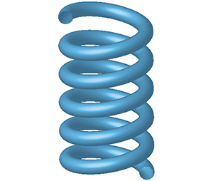
  $2 {\rm \pi}l$ (see figure 1a). Here, the centreline helix refers to the locus of the centre of the pipe. The flow is driven by a body force
  $\boldsymbol {f}^{\ast }$, which has dimensional amplitude
  $F$. The choice of forcing is described in § 2.3. We non-dimensionalize the variables as follows:
 \begin{equation} \boldsymbol{f} = \frac{\boldsymbol{f}^{\ast}}{F}, \quad \boldsymbol{u} = \left(\frac{\rho}{F R_p}\right)^{{1}/{2}}\boldsymbol{u}^{\ast}, \quad p = \frac{p^{\ast} - p_a}{F R_p}, \quad \boldsymbol{x} = \frac{\boldsymbol{x}^{\ast}}{R_p}, \quad t = \left(\frac{F}{\rho R_p}\right)^{{1}/{2}} t^{\ast}. \end{equation}
Here,  $p_a$ is the ambient pressure, whereas
  $\boldsymbol {f}$,
  $\boldsymbol {u}$,
  $p$,
$p$,  $\boldsymbol {x}$ and
  $t$ denote the non-dimensional forcing, velocity, pressure, position and time, respectively. Quantities with a star in superscript are dimensional. The equations governing the flow in non-dimensional form are as follows:
 \begin{equation} \left. \begin{aligned} \boldsymbol{\nabla} \boldsymbol{\cdot} \boldsymbol{u} & = 0,\\ \frac{\partial \boldsymbol{u}}{\partial t} + \boldsymbol{u} \boldsymbol{\cdot} \boldsymbol{\nabla} \boldsymbol{u} & = - \boldsymbol{\nabla} p + \frac{1}{Re} \nabla^2 \boldsymbol{u} + \boldsymbol{f}, \end{aligned} \right\} \end{equation}
where
 \begin{equation} Re = \frac{R_p}{\nu} \left(\frac{F R_p}{\rho}\right)^{{1}/{2}} \end{equation}
is the Reynolds number. The boundary conditions at the surface of the pipe are no-slip and impermeable.

Figure 1.  $(a)$ Schematic diagram of a helical pipe with radius
  $R_p$, radius of the centreline helix
  $R_h$ and pitch of the centreline helix
  $2 {\rm \pi}l$. The dashed line is the axis of rotation of the helical pipe.
  $(b)$ Illustration of the coordinate system
  $(s, r, \phi )$ used in this paper.
2.2. Coordinate system
In this subsection, we construct an orthogonal coordinate system that is well suited to our problem. This coordinate system was first introduced by Germano (Reference Germano1982), who was interested in the effect of small torsion on Dean's solution. The coordinate system has been extensively used since then in both analytical and computational studies of flows in helical pipes (Kao Reference Kao1987; Germano Reference Germano1989; Tuttle Reference Tuttle1990; Liu & Masliyah Reference Liu and Masliyah1993; Yamamoto et al. Reference Yamamoto, Yanase and Yoshida1994; Gammack & Hydon Reference Gammack and Hydon2001; Hüttl & Friedrich Reference Hüttl and Friedrich2001). For clarity and self-consistency, we repeat its construction below.
Let  $a$ and
  $2 {\rm \pi}b$ be the non-dimensional centreline helix radius and pitch, where
  $a = R_h / R_p$ and
  $b = l / R_p$. The equation of this helix parameterized with arc length
  $s$ in a Cartesian coordinate system
  $(x, y, z)$ is given by
 \begin{equation} (x(s), y(s), z(s)) = \left(a \cos\left(\frac{s}{\sqrt{a^2 + b^2}}\right), a \sin\left(\frac{s}{\sqrt{a^2 + b^2}}\right), \frac{b s}{\sqrt{a^2 + b^2}}\right). \end{equation}
Let  $\boldsymbol {R}(s) = (x(s), y(s), z(s))$ be the position vector, and let
  $\boldsymbol {T}(s)$,
  $\boldsymbol {N}(s)$ and
  $\boldsymbol {B}(s)$ be the tangent, normal and binormal to the centreline helix, which are given by
 \begin{equation} \boldsymbol{T} = \frac{\textrm{d} \boldsymbol{R}}{\textrm{d}s}, \quad \boldsymbol{N} = \frac{1}{\kappa} \frac{\textrm{d} \boldsymbol{T}}{\textrm{d} s}, \quad \boldsymbol{B} = \boldsymbol{T} \times \boldsymbol{N}. \end{equation}
The relations among the tangent, normal and binormal are given by the Frenet–Serret formulae, which are
 \begin{equation} \frac{\textrm{d} \boldsymbol{N}}{\textrm{d} s} = \tau \boldsymbol{B} - \kappa \boldsymbol{T}, \quad \frac{\textrm{d} \boldsymbol{B}}{\textrm{d} s} = - \tau \boldsymbol{N}, \end{equation}
where
 \begin{equation} \kappa = \frac{a}{a^2 + b^2} \quad \text{and} \quad \tau = \frac{b}{a^2 + b^2} \end{equation}
are the non-dimensional curvature and torsion of the helix. The curvature is taken smaller than one ( $\kappa < 1$) in this paper. We now construct a coordinate system
  $(s, r, \eta )$ such that any Cartesian position vector
  $\boldsymbol {x}$ can be expressed as
 \begin{equation} \boldsymbol{x} = \boldsymbol{R} + r \cos \eta \boldsymbol{N} + r \sin \eta \boldsymbol{B}. \end{equation}
With the use of (2.5a–c) and (2.6a,b),
 \begin{equation} \textrm{d} \boldsymbol{x} \boldsymbol{\cdot} \textrm{d} \boldsymbol{x} = [(1 - r \kappa \cos \eta)^2 + \tau^2 r^2]\,\textrm{d}s^2 + \textrm{d}r^2 + r^2\,\textrm{d}\eta^2 + 2 \tau r^2\,\textrm{d}s\,\textrm{d}\eta. \end{equation}
Therefore, the resulting coordinate system is non-orthogonal. However, using the transformation  $\eta = \phi - \tau s$ in (2.9), we obtain
 \begin{equation} \textrm{d} \boldsymbol{x} \boldsymbol{\cdot} \textrm{d} \boldsymbol{x} = (1 - r \kappa \cos(\phi - \tau s))^2\,\textrm{d}s^2 + \textrm{d}r^2 + r^2\,\textrm{d}\phi^2. \end{equation}
The coordinate system  $(s, r, \phi )$ is orthogonal, and will be used to perform calculations in the rest of the paper. The scale factors for this coordinate system are defined as
 \begin{equation} h_s = (1 - r \kappa \cos(\phi - \tau s)), \quad h_r = 1, \quad h_{\phi} = r. \end{equation}
 The impermeability and no-slip condition at the surface of the pipe in the  $(s, r, \phi )$ coordinate system translate to
 \begin{equation} \boldsymbol{u} = (u_s, u_r, u_{\phi}) = \boldsymbol{0}\quad \text{at}\ r = 1. \end{equation}
In this paper, we assume that the flow is periodic in the streamwise direction  $s$ with period
  $s_p$. Hence, the domain of interest in the
  $(s, r, \phi )$ coordinate system is
 \begin{equation} \varOmega = [0, s_p]\times[0, 1]\times[0, 2{\rm \pi}]. \end{equation}
2.3. Choice of forcing
We choose to drive the flow with a dimensional forcing
 \begin{equation} \boldsymbol{f}^{\ast} = -\frac{1}{1 - r^{\ast} \kappa^{\ast} \cos(\phi^{\ast} - \tau^{\ast} s^{\ast})} \times \frac{\textrm{d} P}{\textrm{d} s^{\ast}} \ \boldsymbol{e}_{s} \quad \text{for}\ 0 \leq r^{\ast} \leq R_p. \end{equation}
Here,  $-\textrm {d} P/\textrm {d} s^{\ast }$ is a constant and can be thought of as the applied pressure gradient. Note how this streamwise directed forcing varies across the cross-section. The reason for this choice of forcing over a conventional forcing, which would be constant across the cross-section, is that the line integral along the streamwise direction for this forcing is independent of the position on the pipe cross-section and depends only on the difference of streamwise coordinates; i.e.
 \begin{equation} \int_{s^{\ast} = s_1^{\ast}}^{s_2^{\ast}} \boldsymbol{f}^{\ast} \boldsymbol{\cdot} \boldsymbol{e}_{s} \, \textrm{d}l = \int_{s^{\ast} = s_1^{\ast}}^{s_2^{\ast}} - \frac{\textrm{d} P}{\textrm{d} s^{\ast}} \, \textrm{d}s^{\ast} = -\frac{\textrm{d} P}{\textrm{d} s^{\ast}} (s_2^{\ast} - s_1^{\ast}), \end{equation}
where  $\textrm {d} l = h^{\ast }_s\,\textrm {d}s^{\ast }$ is the line element with
  $h^{\ast }_s = 1 - r^{\ast } \kappa ^{\ast } \cos (\phi ^{\ast } - \tau ^{\ast } s^{\ast })$. By contrast, for the conventional forcing, the value of this line integral would also depend on the position on the cross-section. Hence, we believe that our choice of forcing is good for modelling a flow driven by constant-pressure boundary conditions. More detail on this choice of forcing in the context of flow in a torus can be found in Canton et al. (Reference Canton, Schlatter and Örlü2016), Canton, Örlü & Schlatter (Reference Canton, Örlü and Schlatter2017) and Rinaldi, Canton & Schlatter (Reference Rinaldi, Canton and Schlatter2019). Note that in the limit of vanishing curvature (
 $\kappa \to 0$), our choice does reduce to constant forcing in the streamwise direction and therefore is consistent with the usual modelling of pressure-driven flow in a straight pipe. Based on (2.14), we define the forcing scale as
 \begin{equation} F = -\frac{\textrm{d} P}{\textrm{d} s^{\ast}}. \end{equation}
This implies that the non-dimensional forcing is given by
 \begin{equation} \boldsymbol{f} = \frac{1}{1 - r \kappa \cos(\phi - \tau s)} \boldsymbol{e}_{s} \quad \text{for}\ 0 \leq r \leq 1. \end{equation}
2.4. Quantities of interest
We are interested in obtaining a lower bound on the average non-dimensional flow rate  $Q$, which we simply call flow rate, and an equivalent upper bound on the friction factor
  $\lambda$ in the limit of high Reynolds number. As we are concerned with the high-Reynolds-number limit, we use an inertial scaling to define the non-dimensional flow rate
  $Q$ as
 \begin{equation} Q = \frac{1}{R_p^2} \left(\frac{\rho}{F R_p}\right)^{{1}/{2}} Q^{\ast} = \left\langle \int_{\phi = 0}^{2 {\rm \pi}} \int_{r = 0}^{1} u_s r\,\textrm{d}r\,\textrm{d}\phi \right\rangle, \end{equation}
where  $Q^{\ast }$ is the long-time average of the dimensional flow rate,
  $u_s$ is the streamwise component of the non-dimensional velocity field
  $\boldsymbol {u}$ and
 \begin{equation} \langle [ \, \cdot \, ] \rangle = \lim_{T \to \infty} \frac{1}{T} \int_{t = 0}^{T} [\, \cdot \, ] \, \textrm{d}t \end{equation}
denotes the long-time average of a quantity. The Darcy–Weisbach friction factor  $\lambda$, which is four times the Fanning friction factor, is defined as
 \begin{equation} \lambda = - \frac{\textrm{d} P}{\textrm{d} s^{\ast}} \ \frac{4 R_p}{\rho u_m^{\ast 2}}, \end{equation}
where  $u_m^{\ast }$ is the dimensional streamwise mean velocity, given by
 \begin{equation} u_m^{\ast} = \frac{Q^{\ast}}{{\rm \pi} R_p^2}. \end{equation}
When expressed in non-dimensional variables, the friction factor is
 \begin{equation} \lambda = \frac{4 {\rm \pi}^2}{Q^2}. \end{equation}
From (2.22), we notice that a lower bound on the flow rate  $Q$ will provide an upper bound on the friction factor
  $\lambda$.
3. The background method formulation
In this section, we describe the general approach of the background method applied to our problem. The formulation that we develop here is for any general background flow field and is similar to the one given in Constantin & Doering (Reference Constantin and Doering1995) for pressure-driven channel flow.
The background method, in essence, works as follows. We derive time-averaged integral identities from the governing equations (2.2a,b) (using the fact that the long-time averages of certain time derivatives vanish) in order to rewrite the quantity of interest  $Q$ given by (2.18) as an equivalent long-time averaged expression that is easier to bound using analysis techniques. To that end, we begin by establishing a time-averaged total energy equation, by taking the dot product of (2.2b) with
  $\boldsymbol {u}$ and then performing a volume integration on the resulting equation. The result is
 \begin{equation} \frac{1}{2}\frac{\textrm{d} \|\boldsymbol{u}\|^2_2}{\textrm{d} t} = - \frac{1}{Re} \| \boldsymbol{\nabla} \boldsymbol{u}\|^2_2 + \int_{\varOmega} \boldsymbol{f} \boldsymbol{\cdot} \boldsymbol{u} \, \textrm{d} \boldsymbol{x}, \end{equation}
where  $\|\cdot \|_2$ denotes the
  $L^2$-norm, which is given by
 \begin{equation} \|\cdot\|_2 = \left(\int_{\varOmega} |\cdot|^2 \, \textrm{d} \boldsymbol{x}\right)^{{1}/{2}}, \end{equation}
and where the volume integral in  $(s, r, \phi )$ coordinates is written as
 \begin{equation} \int_{\varOmega} [\, \cdot \, ] \, \textrm{d} \boldsymbol{x} = \int_{s = 0}^{s_p} \int_{\phi = 0}^{2 {\rm \pi}} \int_{r = 0}^{1} [\, \cdot \, ] \ h_s h_r h_{\phi}\,\textrm{d}r\,\textrm{d}\phi\,\textrm{d}s. \end{equation}
The quantity  $\|\boldsymbol {u}\|_2^2(t)$ can be shown to be uniformly bounded in time within the framework of the background method (see, for example, Doering & Constantin (Reference Doering and Constantin1992) and Constantin & Doering (Reference Constantin and Doering1995)). Therefore, the long-time average of the time derivative of
  $\|\boldsymbol {u}\|_2^2(t)$ vanishes. As a result, taking the long-time average of (3.1) leads to
 \begin{equation} \left\langle \int_{\varOmega} \boldsymbol{f} \boldsymbol{\cdot} \boldsymbol{u} \, \textrm{d} \boldsymbol{x} \right\rangle = \frac{1}{Re} \langle \|\boldsymbol{\nabla} \boldsymbol{u}\|^2_2 \rangle . \end{equation}
The second step of the method is to perform the background decomposition. We start by writing the total velocity  $\boldsymbol {u}$ as the sum of two divergence-free velocity fields
  $\boldsymbol {u} = \boldsymbol {U} + \boldsymbol {v}$, where
  $\boldsymbol {\nabla } \boldsymbol {\cdot } \boldsymbol {U} = 0$ and
  $\boldsymbol {\nabla } \boldsymbol {\cdot } \boldsymbol {v} = 0$. We call
  $\boldsymbol {U}$ the background flow, which is steady and satisfies the same boundary conditions as the full flow
  $\boldsymbol {u}$, while the perturbation
  $\boldsymbol {v}$ satisfies the homogeneous version of the boundary conditions. The equation governing the evolution of
  $\boldsymbol {v}$ is given by
 \begin{equation} \frac{\partial \boldsymbol{v}}{\partial t} + \boldsymbol{U} \boldsymbol{\cdot} \boldsymbol{\nabla} \boldsymbol{U} + \boldsymbol{U} \boldsymbol{\cdot} \boldsymbol{\nabla} \boldsymbol{v} + \boldsymbol{v} \boldsymbol{\cdot} \boldsymbol{\nabla} \boldsymbol{U} + \boldsymbol{v} \boldsymbol{\cdot} \boldsymbol{\nabla} \boldsymbol{v} = - \boldsymbol{\nabla} p + \frac{1}{Re} \nabla^2 \boldsymbol{U} + \frac{1}{Re} \nabla^2 \boldsymbol{v} + \boldsymbol{f}. \end{equation}
Taking the dot product of the above equation with  $\boldsymbol {v}$ and performing a volume integration, then taking the long-time average, results in
 \begin{equation} \left\langle \int_{\varOmega} \boldsymbol{f} \boldsymbol{\cdot} \boldsymbol{v} \, \textrm{d} \boldsymbol{x} \right\rangle = \frac{1}{2 Re} \langle \|\boldsymbol{\nabla} \boldsymbol{u}\|_2^2 \rangle - \frac{1}{2 Re} \|\boldsymbol{\nabla} \boldsymbol{U}\|_2^2 + \langle \mathcal{H}(\boldsymbol{v}) \rangle , \end{equation}
where
 \begin{equation} \mathcal{H}(\boldsymbol{v}) = \underbrace{\int_{\varOmega} (\boldsymbol{v} \boldsymbol{\cdot} \boldsymbol{\nabla} \boldsymbol{U}_{{sym}}) \boldsymbol{\cdot} \boldsymbol{v} \, \textrm{d} \boldsymbol{x}}_{I} + \underbrace{\int_{\varOmega} (\boldsymbol{U} \boldsymbol{\cdot} \boldsymbol{\nabla} \boldsymbol{U}) \boldsymbol{\cdot} \boldsymbol{v} \, \textrm{d} \boldsymbol{x}}_{II} + \underbrace{\frac{1}{2 Re} \|\boldsymbol{\nabla} \boldsymbol{v}\|_2^2}_{III}, \end{equation}
and  $\boldsymbol {\nabla } \boldsymbol {U}_{{sym}}$ is the symmetric part of
  $\boldsymbol {\nabla } \boldsymbol {U}$, i.e.
 \begin{equation} \boldsymbol{\nabla} \boldsymbol{U}_{{sym}} = \frac{\boldsymbol{\nabla} \boldsymbol{U} + \boldsymbol{\nabla} \boldsymbol{U}^{\intercal}}{2}. \end{equation}
We have used the following identity in deriving the equation (3.6):
 \begin{equation} |\boldsymbol{\nabla} \boldsymbol{u}|^2 = |\boldsymbol{\nabla} \boldsymbol{U}|^2 + |\boldsymbol{\nabla} \boldsymbol{v}|^2 + 2 \boldsymbol{\nabla} \boldsymbol{U} \boldsymbol{\colon} \boldsymbol{\nabla} \boldsymbol{v}, \end{equation}
where, in index notation,
 \begin{equation} \boldsymbol{\nabla} \boldsymbol{U} \boldsymbol{\colon} \boldsymbol{\nabla} \boldsymbol{v} = \partial_{i} v_j \partial_{i} U_j. \end{equation}
Multiplying (3.6) by two and subtracting (3.4) yields
 \begin{equation} 2 \left\langle \int_{\varOmega} \boldsymbol{f} \boldsymbol{\cdot} \boldsymbol{v} \, \textrm{d} \boldsymbol{x} \right\rangle - \left\langle \int_{\varOmega} \boldsymbol{f} \boldsymbol{\cdot} \boldsymbol{u} \, \textrm{d} \boldsymbol{x} \right\rangle = - \frac{1}{Re} \|\boldsymbol{\nabla} \boldsymbol{U}\|_2^2 + 2 \left\langle\mathcal{H}(\boldsymbol{v})\right\rangle\!. \end{equation}
The left-hand side of (3.11) can be simplified as follows:
 \begin{align} & 2 \left\langle \int_{\varOmega} \boldsymbol{f} \boldsymbol{\cdot} \boldsymbol{v} \, \textrm{d} \boldsymbol{x} \right\rangle - \left\langle \int_{\varOmega} \boldsymbol{f} \boldsymbol{\cdot} \boldsymbol{u} \, \textrm{d} \boldsymbol{x} \right\rangle = \left\langle \int_{\varOmega} \boldsymbol{f} \boldsymbol{\cdot} \boldsymbol{u} \, \textrm{d} \boldsymbol{x} \right\rangle - 2 \left\langle \int_{\varOmega} \boldsymbol{f} \boldsymbol{\cdot} \boldsymbol{U} \, \textrm{d} \boldsymbol{x} \right\rangle\nonumber\\ &\qquad = \left\langle \int_{s = 0}^{s_p} \left[ \int_{\phi = 0}^{2 {\rm \pi}} \int_{r = 0}^{1} u_s r\,\textrm{d}r \,\textrm{d}\phi \right]\,\textrm{d}s \right\rangle - 2 \int_{s = 0}^{s_p} \left[ \int_{\phi = 0}^{2 {\rm \pi}} \int_{r = 0}^{1} U_s r\,\textrm{d}r\,\textrm{d}\phi \right]\,\textrm{d}s\nonumber\\ &\qquad = s_p \left\langle \int_{\phi = 0}^{2 {\rm \pi}} \int_{r = 0}^{1} u_s r\,\textrm{d}r\,\textrm{d}\phi \right\rangle - 2 s_p \int_{\phi = 0}^{2 {\rm \pi}} \int_{r = 0}^{1} U_s r\,\textrm{d}r\,\textrm{d}\phi. \end{align}
Note that we used  $\boldsymbol {v} = \boldsymbol {u} - \boldsymbol {U}$ in the first line, then substituted the expression for
  $\boldsymbol {f}$ from (2.17) and used the time-independence of
  $\boldsymbol {U}$ to obtain the second line. The terms in the square brackets in the second line represent the flow of
  $\boldsymbol {u}$ and
  $\boldsymbol {U}$ through a cross-section of pipe and therefore are independent of the streamwise direction
  $s$ because of the incompressibility of
  $\boldsymbol {u}$ and
  $\boldsymbol {U}$. Hence, we can easily integrate these expressions with respect to
  $s$, which leads to the third line. Using (3.12) in (3.11) and dividing by
  $s_p$ on both sides gives
 \begin{equation} Q = \left\langle \int_{\phi = 0}^{2 {\rm \pi}} \int_{r = 0}^{1} u_s r\,\textrm{d}r\,\textrm{d}\phi \right\rangle = 2 \int_{\phi = 0}^{2 {\rm \pi}} \int_{r = 0}^{1} U_s r\,\textrm{d}r\,\textrm{d}\phi - \frac{1}{s_p Re} \|\boldsymbol{\nabla} \boldsymbol{U}\|_2^2 + \frac{2}{s_p} \langle\mathcal{H}(\boldsymbol{v})\rangle\!. \end{equation}
If one can prove that
 \begin{equation} \mathcal{H}(\boldsymbol{v}) + \gamma \geq 0 \quad \forall \ \boldsymbol{v} \end{equation}
for a background flow  $\boldsymbol {U}$ and some constant
  $\gamma$, then we have the following bound on the flow rate:
 \begin{equation} Q \geq 2 \int_{\phi = 0}^{2 {\rm \pi}} \int_{r = 0}^{1} U_s r \, \textrm{d}r\,\textrm{d}\phi - \frac{1}{s_p Re} \|\boldsymbol{\nabla} \boldsymbol{U}\|_2^2 - \frac{2 \gamma}{s_p}. \end{equation}
Following the convention (Doering & Constantin Reference Doering and Constantin1994; Constantin & Doering Reference Constantin and Doering1995), we call (3.14) the spectral constraint.
Note that the background method formulation given in Constantin & Doering (Reference Constantin and Doering1995) for pressure-driven channel flows assumes that the background flow  $\boldsymbol {U}$ is unidirectional and planar (a choice that is only suitable for planar geometries). As a result, the term
  $II$ in (3.7) is zero and therefore the functional
  $\mathcal {H}(\boldsymbol {v})$ is homogeneous in their work. Here, we have given the background method formulation for a general background flow
  $\boldsymbol {U}$. Also, as we shall see, the choice of background flow which works in the present case is two-dimensional, which leads to a non-zero term
  $II$ in (3.7), and therefore the resultant functional
  $\mathcal {H}(\boldsymbol {v})$ is inhomogeneous.
4. Bounds on flow rate and friction factor
In this section, we obtain a lower bound on the flow rate and an equivalent upper bound on the friction factor. We choose a family of background flows with varying boundary layer thickness along the circumference of the pipe. This variation of the boundary layer thickness will be carefully selected so that the spectral constraint (3.14) is satisfied while the bound (3.15) is optimized simultaneously for different values of curvature  $\kappa$ and torsion
  $\tau$; a geometrical dependence on these parameters will thereby be obtained. Note that in this paper, the boundary layer refers to the term boundary layer used in the context of the background method (see, for instance, Doering & Constantin (Reference Doering and Constantin1994) and Goluskin & Doering (Reference Goluskin and Doering2016)) and is not the conventional viscous boundary layer.
4.1. Choice of background flow
We make the following choice of background flow:
 \begin{align} &\boldsymbol{U}(s, r, \phi)\nonumber\\ &\quad = \begin{cases} \left(\varLambda (1 - r \kappa \cos(\phi - \tau s)), 0, \varLambda \tau r \right) & \text{if}\ 0 \leq r < 1 - \delta g(s, \phi),\\ \left(\varLambda (1 - r \kappa \cos(\phi - \tau s)) \left(\dfrac{1 - r}{\delta g(s, \phi)}\right), 0, \varLambda \tau r \left(\dfrac{1 - r}{\delta g(s, \phi)}\right) \right) & \text{if}\ 1 - \delta g(s, \phi) \leq r \leq 1. \end{cases} \end{align}
Here,  $\varLambda$ is a constant that will be adjusted later to optimize the bound,
 \begin{equation} \delta = \frac{1}{Re} \end{equation}
and  $g(s, \phi )$ is a non-zero bounded differentiable function of
  $s$ and
  $\phi$ that satisfies
 \begin{equation} 0 < g_l \leq g(s, \phi) \leq g_u \quad \text{and} \quad \left|\frac{\partial g}{\partial s}\right|, \left|\frac{\partial g}{\partial \phi}\right| \leq g^{\prime}_u \quad \forall \ s \in [0, s_p], \phi \in [0, 2 {\rm \pi}], \end{equation}
where  $g_l$,
  $g_u$ and
  $g^{\prime }_u$ are constants independent of
  $Re$. The region
  $1 - \delta g(s, \phi ) \leq r \leq 1$ is the boundary layer, denoted by
 \begin{equation} \varOmega_{\delta} = \{(s, r, \phi) | s \in [0, s_p], \phi \in [0, 2 {\rm \pi}], 1 - \delta g(s, \phi) \leq r \leq 1\}, \end{equation}
and the function  $g(s, \phi )$ represents the shape of the boundary layer, which will be determined later as part of the analysis to optimize the bound. Physically, (4.3a,b) means that the thickness of the boundary layer is everywhere non-zero and finite, and it varies smoothly. Figure 2 shows a colour map of the streamwise component
  $U_s$ of the background flow (4.1). It can be easily verified that the background flow field (4.1) satisfies the no-slip and impermeable boundary conditions on the pipe surface. Meanwhile, the divergence-free condition on the background flow enforces
 \begin{equation} g(s, \phi) = g(\phi - \tau s), \end{equation}
which constrains the choice of  $g$. See appendix A for the calculation of divergence of a vector in the
  $(s, r, \phi )$ coordinate system. Also, note that for this choice of
  $\boldsymbol {U}$, in the bulk region (
 $0 \leq r \leq 1 - \delta g(s, \phi )$) we have
 \begin{equation} \boldsymbol{\nabla} \boldsymbol{U}_{{sym}} = \boldsymbol{\mathsf{0}} \end{equation}
(see appendix C), the reason being that in this region  $\boldsymbol {U}$ is really a rigid body flow as viewed from some inertial frame of reference (see § 5). Although we can obtain a bound on the flow rate with a constant boundary layer thickness, this choice does not provide the optimal bound as a function of the pipe's curvature
  $\kappa$ and torsion
  $\tau$. Unlike the case of planar geometries, the choice of the background flow (4.1) is not uniform in the bulk region. As can be seen in figure 2, the magnitude of the streamwise component
  $U_s$ of the background flow in the bulk region varies and is higher towards the outer edge O of the pipe than the inner edge. This means that a constant boundary layer thickness is not necessarily the optimal choice for every
  $\kappa$ and
  $\tau$. Therefore, it is natural to choose a variable boundary layer thickness (which is more general than the choice of constant boundary layer thickness), since our goal is to optimize bounds simultaneously for different values of curvature and torsion. Furthermore, in the process of obtaining bounds, we complement this choice of variable boundary layer thickness with inequalities suitably constructed (from standard analysis inequalities) to achieve this goal. In the forthcoming analysis, we will be interested in obtaining a bound in the limit of high Reynolds number and therefore will frequently be making use of the fact that
  $Re \gg 1$ or
  $\delta \ll 1$ to retain only the leading-order terms.

Figure 2. Variation of the streamwise component  $U_s$ of the background flow (4.1) across a cross-section of the pipe. In this example, the pipe's curvature is
  $\kappa = 0.5$ and its torsion is
  $\tau = 0.25$. The solid black curve shows the edge of the boundary layer with variable thickness
  $\delta g(s, \phi )$. The point
  $O$ denotes the outer edge of the pipe, i.e. the point on the cross-section which is farthest from the axis of rotation of the helical pipe. The background flow in this figure corresponds to
  $\varLambda = 1$, and the boundary layer shape
  $g(s, \phi )$ is given by (4.21a–c), which is the shape obtained in the process of optimizing the bound.
4.2. The spectral constraint
In this subsection, we use analysis techniques to obtain a condition under which the spectral constraint (3.14) is satisfied. In what follows, we shall make use of a crucial inequality, whose proof is given in appendix B.
Inequality Let  $w:\varOmega _{\delta } \to \mathbb {R}$ be a square-integrable function such that
  $w(s, 1, \phi ) = 0$ for all
  $0 \leq s \leq s_p$ and
  $0 \leq \theta \leq 2 {\rm \pi}$; then the following statement is true:
 \begin{equation} \int_{\varOmega_{\delta}} \sigma w^2 \, \textrm{d} \boldsymbol{x} \leq \frac{\delta^2}{2}\int_{\varOmega_{\delta}} \sigma (s, 1, \phi) g^2(s, \phi) \left(\frac{\partial w}{\partial r}\right)^2 \, \textrm{d} \boldsymbol{x} + O(\delta^3) \ \|\boldsymbol{\nabla} w\|_2^2. \end{equation}
Here,  $\sigma :\varOmega _{\delta } \to \mathbb {R}$ is a positive bounded
  $O(1)$ function that satisfies
 \begin{equation} |\sigma (s, r, \phi) - \sigma (s, 1, \phi)| = O(\delta) \quad \text{for}\ (s, r, \phi) \in \varOmega_{\delta}. \end{equation}
 For convenience, we make use of the big-O notation  $O(\cdot )$. Let
  $m$ and
  $n$ be two functions; then in this notation, writing
  $m(\delta ) = O(n(\delta ))$ means that there exist two positive constants
  $C > 0$ and
  $\delta _0 > 0$ such that
  $|m(\delta )| \leq C |n(\delta )|$ whenever
  $0 \leq \delta < \delta _0$.
We start by obtaining a bound on  $I$ as defined in (3.7). Making use of (4.6) leads to
 \begin{equation} I = \int_{\varOmega} (\boldsymbol{v} \boldsymbol{\cdot} \boldsymbol{\nabla} \boldsymbol{U}_{{sym}}) \boldsymbol{\cdot} \boldsymbol{v} \, \textrm{d} \boldsymbol{x} = \int_{\varOmega_{\delta}} (\boldsymbol{v} \boldsymbol{\cdot} \boldsymbol{\nabla} \boldsymbol{U}_{{sym}}) \boldsymbol{\cdot} \boldsymbol{v} \, \textrm{d} \boldsymbol{x}. \end{equation}
The following inequality is obtained by substituting  $\boldsymbol {\nabla } \boldsymbol {U}_{{sym}}$ (which can be calculated using (C 2) from appendix C) into (4.9):
 \begin{align} |I| &\leq \int_{\varOmega_{\delta}} \xi_1(s, r, \phi) |v_s| |v_r| \, \textrm{d} \boldsymbol{x} + \int_{\varOmega_{\delta}} \xi_2(s, r, \phi) |v_{\phi}| |v_r|\, \textrm{d} \boldsymbol{x} \nonumber\\ &\qquad + \int_{\varOmega_{\delta}} \xi_3 v_s^2\,\textrm{d} \boldsymbol{x} + \int_{\varOmega_{\delta}} \xi_4 v_{\phi}^2 \, \textrm{d} \boldsymbol{x} + \int_{\varOmega_{\delta}} \xi_5 |v_s| |v_{\phi}| \, \textrm{d} \boldsymbol{x} , \end{align}
where
 \begin{align} \left. \begin{aligned} & \xi_1(s, r, \phi) = \frac{\varLambda (1 - r \kappa \cos(\phi - \tau s)) }{\delta g}, \quad \xi_2(s, r, \phi) = \frac{\varLambda \tau r}{\delta g},\\ & \xi_3 = \max_{(s, r, \phi) \in \varOmega_{\delta}}\frac{\varLambda (1-r)}{\delta g^2} \left|\frac{\partial g}{\partial s}\right|, \quad \xi_4 = \max_{(s, r, \phi) \in \varOmega_{\delta}} \frac{\varLambda \tau (1-r)}{\delta g^2} \left|\frac{\partial g}{\partial \phi}\right|,\\ & \xi_5 = \max_{(s, r, \phi) \in \varOmega_{\delta}} \frac{\varLambda (1-r)}{\delta g^2} \left[\frac{\tau r}{(1 - r \kappa \cos(\phi - \tau s))} \left|\frac{\partial g}{\partial s}\right| + \frac{(1 - r \kappa \cos(\phi - \tau s))}{r} \left|\frac{\partial g}{\partial \phi}\right|\right]. \end{aligned} \right\} \end{align}
Given that  $1-r$ is
  $O(\delta )$ in the boundary layer, and using the constraints on
  $g$ and its derivatives from (4.3a,b), we deduce that
  $\xi _3$,
  $\xi _4$ and
  $\xi _5$ are
  $O(1)$ constants. Using Young's inequality
  $|v_s| |v_{\phi }| \leq (|v_s|^2 + |v_{\phi }|^2)/2$, the last three integrals in (4.10) can be replaced by
 \begin{equation} \int_{\varOmega_{\delta}} \left(\xi_3 + \frac{\xi_5}{2}\right) v_s^2\,\textrm{d} \boldsymbol{x} + \int_{\varOmega_{\delta}} \left(\xi_4 + \frac{\xi_5}{2}\right) v_{\phi}^2 \, \textrm{d} \boldsymbol{x}. \end{equation}
An application of Inequality 4.1 to these two integrals with  $w = v_s$ in the first integral,
  $w = v_{\phi }$ in the second integral and
  $\sigma$ taken to be an
  $O(1)$ constant in both cases produces the following bound on
  $I$:
$I$:
 \begin{equation} |I| \leq \int_{\varOmega_{\delta}} \xi_1(s, r, \phi) |v_s| |v_r| \, \textrm{d} \boldsymbol{x} + \int_{\varOmega_{\delta}} \xi_2(s, r, \phi) |v_{\phi}| |v_r|\, \textrm{d} \boldsymbol{x} + O(\delta^2) \|\boldsymbol{\nabla} \boldsymbol{v}\|_2^2. \end{equation}
In a similar manner, we obtain bounds on the remaining two integrals in (4.13). These bounds contribute to the leading-order term of the bound on  $|I|$; therefore, this time we perform the computation wisely with the intent of optimizing the bound on
  $|I|$ simultaneously in
  $\kappa$ and
  $\tau$. We use the following inequalities (based on Young's inequality) in (4.13):
 \begin{equation} |v_s| |v_r| \leq \frac{c_1(s, \phi) |v_s|^2}{2} + \frac{|v_r|^2}{2 c_1(s, \phi)}, \quad |v_{\phi}| |v_r| \leq \frac{c_2(s, \phi) |v_{\phi}|^2}{2} + \frac{|v_r|^2}{2 c_2(s, \phi)}, \end{equation}
where
 \begin{equation} 0 < c_1(s, \phi) \quad \text{and} \quad 0 < c_2(s, \phi). \end{equation}
This results in
 \begin{align} & |I| \leq \int_{\varOmega_{\delta}} \left[\frac{c_1(s, \phi) \xi_1(s, r, \phi)}{2}\right] |v_s|^2 \, \textrm{d} \boldsymbol{x} + \int_{\varOmega_{\delta}} \left[\frac{\xi_1(s, r, \phi)}{2 c_1(s, \phi)} + \frac{\xi_2(s, r, \phi)}{2 c_2(s, \phi)}\right] |v_r|^2 \, \textrm{d} \boldsymbol{x}\nonumber\\ &\qquad + \int_{\varOmega_{\delta}} \left[\frac{c_2(s, \phi) \xi_2(s, r, \phi)}{2}\right] |v_{\phi}|^2 \, \textrm{d} \boldsymbol{x} + O(\delta^2) \|\boldsymbol{\nabla} \boldsymbol{v}\|_2^2. \end{align}
We apply Inequality 4.1 to the three integrals in (4.16) with  $w=v_s$,
  $w=v_r$ and
  $w=v_{\phi }$, taking
  $\sigma$ to be the corresponding terms in the square brackets times
  $\delta$, which yields
 \begin{equation} |I| \leq \frac{\varLambda \delta}{4} \left[ \int_{\varOmega_{\delta}} p_1 \left(\frac{\partial v_s}{\partial r}\right)^2 \, \textrm{d} \boldsymbol{x} \!+\! \int_{\varOmega_{\delta}} p_2 \left(\frac{\partial v_r}{\partial r}\right)^2 \, \textrm{d} \boldsymbol{x} + \int_{\varOmega_{\delta}} p_3 \left(\frac{\partial v_{\phi}}{\partial r}\right)^2 \, \textrm{d} \boldsymbol{x}\right] + O(\delta^2) \|\boldsymbol{\nabla} \boldsymbol{v}\|_2^2, \end{equation}
where
 \begin{equation} \left. \begin{aligned} p_1 & = (1-\kappa \cos(\phi - \tau s)) g(s, \phi) c_1(s, \phi), \\ p_2 & = \frac{ (1-\kappa \cos(\phi - \tau s)) g(s, \phi) }{ c_1(s, \phi)} + \frac{ \tau g(s, \phi) }{ c_2(s, \phi)}, \\ p_3 & = \tau g(s, \phi) c_2(s, \phi). \end{aligned} \right\} \end{equation}
We now choose the functions  $g(s, \phi )$,
  $c_1(s, \phi )$ and
  $c_2(s, \phi )$ so that
  $p_1$,
  $p_2$ and
  $p_3$ are constants. For this choice, the bound on
  $I$ can be written as
 \begin{equation} |I| \leq \frac{\varLambda \delta}{4} \max \{p_1, p_2, p_3\} \ \|\boldsymbol{\nabla} \boldsymbol{v}\|_2^2 + O(\delta^2) \|\boldsymbol{\nabla} \boldsymbol{v}\|_2^2. \end{equation}
To optimize the bound, we need
 \begin{equation} p_1 = p_2 = p_3, \end{equation}
as shown in appendix C. Combining this condition with the requirement that  $p_1, p_2,$ and
  $p_3$ should be constants leads to
 \begin{align} \left. \begin{aligned} g(s, \phi) & = \frac{g_c}{\sqrt{(1-\kappa \cos(\phi - \tau s))^2 + \tau^2}},\\ c_1(s, \phi) & = \sqrt{1 + \frac{\tau^2}{(1-\kappa \cos(\phi - \tau s))^2}}, \quad c_2(s, \phi) = \sqrt{1 + \frac{(1-\kappa \cos(\phi - \tau s))^2}{\tau^2}}, \end{aligned} \right\} \end{align}
with  $g_c$ being an
  $O(1)$ positive constant. Note that the function
  $g(s, \phi )$ satisfies the constraints (4.3a,b) and (4.5), where the constants
  $g_l$,
  $g_u$,
  $g_u^{\prime }$ in (4.3a,b) can be chosen as
 \begin{equation} g_l = \frac{g_c}{\sqrt{(1+\kappa)^2 + \tau^2}}, \quad g_u = \frac{g_c}{\sqrt{(1-\kappa)^2 + \tau^2}}, \quad g_u^{\prime} = \frac{2 g_c }{[(1-\kappa)^2 + \tau^2]^{3/2}}. \end{equation}
Combining (4.18a–c), (4.19) and (4.21a–c) gives the following bound on  $I$:
$I$:
 \begin{equation} |I| \leq \left|\int_{\varOmega} \boldsymbol{v} \boldsymbol{\cdot} \boldsymbol{\nabla} \boldsymbol{U} \boldsymbol{\cdot} \boldsymbol{v} \, \textrm{d} \boldsymbol{x}\right| \leq \left(\frac{\varLambda g_c \delta}{4} + O(\delta^2)\right) \|\boldsymbol{\nabla} \boldsymbol{v}\|_2^2. \end{equation}
Next, we show that the contribution of term  $II$, as defined in (3.7), is of higher order in
  $\delta$ than that of term
  $I$. First note that for any scalar function
  $\varPsi$,
 \begin{equation} II = \int_{\varOmega} \boldsymbol{U} \boldsymbol{\cdot} \boldsymbol{\nabla} \boldsymbol{U} \boldsymbol{\cdot} \boldsymbol{v} \, \textrm{d} \boldsymbol{x} = \int_{\varOmega} (\boldsymbol{U} \boldsymbol{\cdot} \boldsymbol{\nabla} \boldsymbol{U} - \boldsymbol{\nabla} \varPsi) \boldsymbol{\cdot} \boldsymbol{v} \, \textrm{d} \boldsymbol{x} \end{equation}
by the incompressibility of  $\boldsymbol {v}$ together with the fact that
  $\boldsymbol {v}$ satisfies the homogeneous boundary conditions. Then, if we choose
  $\varPsi$ such that
  $\boldsymbol {U} \boldsymbol {\cdot } \boldsymbol {\nabla } \boldsymbol {U} = \boldsymbol {\nabla } \varPsi$ in
  $\varOmega \setminus \varOmega _{\delta }$, that is,
 \begin{equation} \varPsi(s, r, \phi) = \varLambda^2 \kappa \cos(\phi - \tau s) \left(r - \frac{r^2}{2} \kappa \cos(\phi - \tau s)\right) - \frac{\varLambda^2 \tau^2 r^2}{2}, \end{equation}
then one can readily check that
 \begin{align} |(\boldsymbol{U} \boldsymbol{\cdot} \boldsymbol{\nabla} \boldsymbol{U} - \boldsymbol{\nabla} \varPsi)| (\boldsymbol{x}) = \begin{cases} 0 & \text{if}\ \boldsymbol{x} \in \varOmega \setminus \varOmega_{\delta}, \\ O(1) & \text{if}\ \boldsymbol{x} \in \varOmega_{\delta}. \end{cases} \end{align}
See appendix C for the calculation of  $\boldsymbol {\nabla } \boldsymbol {U}$. Using (4.26), we can finally obtain a bound on
  $II$ as
 \begin{align} |II| & = \left|\int_{\varOmega} \boldsymbol{U} \boldsymbol{\cdot} \boldsymbol{\nabla} \boldsymbol{U} \boldsymbol{\cdot} \boldsymbol{v} \, \textrm{d} \boldsymbol{x}\right| = \left|\int_{\varOmega} (\boldsymbol{U} \boldsymbol{\cdot} \boldsymbol{\nabla} \boldsymbol{U} - \boldsymbol{\nabla} \varPsi) \boldsymbol{\cdot} \boldsymbol{v} \, \textrm{d} \boldsymbol{x}\right|\nonumber\\ \implies |II| & \leq O(1) \int_{\varOmega_{\delta}} |\boldsymbol{v}| \, \textrm{d} \boldsymbol{x} \nonumber\\ & \leq O(1) \int_{\varOmega_{\delta}} |\boldsymbol{v}|^2 \, \textrm{d} \boldsymbol{x} + O(1) \int_{\varOmega_{\delta}} 1 \, \textrm{d} \boldsymbol{x} \nonumber\\ & \leq O(\delta^{2}) \|\boldsymbol{\nabla} \boldsymbol{v}\|_2^2 + s_p O(\delta). \end{align}
We have used Young's inequality to obtain the third line and Inequality 4.1 to obtain the last line. Finally, using the triangle inequality and the bounds derived on  $I$ and
  $II$, we obtain a bound on the quantity
  $\mathcal {H}(\boldsymbol {v})$ defined in (3.7),
 \begin{equation} \mathcal{H}(\boldsymbol{v}) \geq \frac{1}{2 Re} \|\boldsymbol{\nabla} \boldsymbol{v}\|_2^2 - \left(\frac{\varLambda g_c \delta}{4} + O(\delta^2)\right) \|\boldsymbol{\nabla} \boldsymbol{v}\|_2^2 - s_p O(\delta), \end{equation}
which implies
 \begin{equation} \mathcal{H}(\boldsymbol{v}) + \gamma \geq 0 \end{equation}
as long as
 \begin{equation} g_c \leq \frac{2}{\varLambda} + O(\delta) \quad \text{and} \quad \gamma = s_p O(\delta). \end{equation}
4.3. Bounds on mean quantities
We are now ready to compute the bound on the flow rate. We begin by evaluating the first term on the right-hand side of (3.15) as
 \begin{align} & \int_{\phi = 0}^{2 {\rm \pi}} \int_{r = 0}^{1} U_s r\,\textrm{d}r\,\textrm{d}\phi = \int_{\phi = 0}^{2 {\rm \pi}} \int_{r = 0}^{1 - \delta g(s, \phi)} \varLambda (1 - r \kappa \cos(\phi - \tau s)) r\,\textrm{d}r\,\textrm{d}\phi \nonumber\\ &\qquad\quad + \int_{\phi = 0}^{2 {\rm \pi}} \int_{1 - \delta g(s, \phi)}^{1} \varLambda (1 - r \kappa \cos(\phi - \tau s)) \frac{(1-r)}{\delta g} r\,\textrm{d}r\,\textrm{d}\phi \nonumber\\ &\qquad = \int_{\phi = 0}^{2 {\rm \pi}} \int_{r = 0}^{1} \varLambda (1 - r \kappa \cos(\phi - \tau s)) r \,\textrm{d}r\,\textrm{d}\phi + O(\delta) \nonumber\\ &\qquad = {\rm \pi}\varLambda + O(\delta). \end{align}
Similarly, the second term on the right-hand side of (3.15) is as follows:
 \begin{align} \|\boldsymbol{\nabla} \boldsymbol{U}\|_2^2 & = \int_{\varOmega_{\delta}} |\boldsymbol{\nabla} \boldsymbol{U}|^2 \, \textrm{d} \boldsymbol{x} + \int_{\varOmega \setminus \varOmega_{\delta}} |\boldsymbol{\nabla} \boldsymbol{U}|^2 \, \textrm{d} \boldsymbol{x} \nonumber\\ & = \int_{s = 0}^{s_p} \int_{\phi = 0}^{2 {\rm \pi}} \int_{1 - \delta g(s, \phi)}^{1} |\boldsymbol{\nabla} \boldsymbol{U}|^2 \ h_s h_r h_{\phi}\,\textrm{d}r\,\textrm{d} \phi\,\textrm{d}s + s_p O(1) \nonumber\\ & = \frac{2 {\rm \pi}\varLambda^2 s_p}{\delta \; g_c} I(\kappa, \tau) + s_p O(1), \end{align}
where
 \begin{equation} I(\kappa, \tau) = \frac{1}{2 {\rm \pi}}\int_{0}^{2 {\rm \pi}} ((1-\kappa \cos \alpha)^2 + \tau^2)^{3/2}(1-\kappa \cos \alpha) \, \textrm{d} \alpha. \end{equation}
The integrand in the second line of (4.32) is explicitly calculated in (C 4); see appendix C. Using (4.31) and (4.32) in (3.15), we obtain a bound on the flow rate  $Q$ as
 \begin{equation} Q \geq 2 {\rm \pi}\varLambda - \frac{2 {\rm \pi}\varLambda^2}{g_c} I(\kappa, \tau) + O(\delta). \end{equation}
We see that choosing a small value of  $g_c$ will make the bound on
  $Q$ worse. Therefore, to obtain the best possible bound, we choose the largest possible value of
  $g_c$ which satisfies the constraint (4.30), i.e.
 \begin{equation} g_c = \frac{2}{\varLambda} + O(\delta). \end{equation}
The bound on  $Q$ then reads
 \begin{equation} Q \geq 2 {\rm \pi}\varLambda - {\rm \pi}\varLambda^3 I(\kappa, \tau) + O(\delta). \end{equation}
All that remains is to choose  $\varLambda$ to maximize this lower bound. The optimal value of
  $\varLambda$ is given by
 \begin{equation} \varLambda = \sqrt{\frac{2}{3 I(\kappa, \tau)}}. \end{equation}
Substituting (4.37) into (4.36) and using  $\delta = 1/Re$ as defined earlier in (4.2) gives a bound on the flow rate as
 \begin{equation} Q \geq \sqrt{\frac{32 {\rm \pi}^2}{27 I(\kappa, \tau)}} + O(Re^{-1}). \end{equation}
 Using this lower bound, together with the definition (2.22) of the friction factor  $\lambda$ in terms of
  $Q$, we finally obtain an upper bound on the friction factor as
 \begin{equation} \lambda \leq \lambda_b = \frac{27}{8} I(\kappa, \tau) + O(Re^{-1}). \end{equation}
 These bounds on the flow rate (4.38) and friction factor (4.39) are also valid for a toroidal ( $\kappa \neq 0, \tau = 0$) or a straight (
 $\kappa = 0, \tau = 0$) pipe. In general, the integral
  $I(\kappa , \tau )$ cannot be obtained analytically except when
  $\tau$ is zero or small. Table 1 summarizes the bounds derived on the flow rate and friction factor in different limits of curvature and torsion. For a toroidal pipe, a small radius of curvature has a second-order effect on the bounds (see table 1), which is also the case in the exact solution for the flow at low Reynolds number (see Dean Reference Dean1928). Similarly, for a helical pipe, the effect of a small torsion is of second order on our bounds, and as before, this is the case for the steady-state solution at low Reynolds number (see Tuttle Reference Tuttle1990). More generally, the effect of increasing curvature and torsion is always to decrease the lower bound on the volume flow rate and to increase the upper bound on the friction factor. For a straight pipe, the bound on the friction factor reduces to
  $\lambda _{b, st} = 27/8$, which is
  $12.5$ times larger than the bound
  $0.27$ (Plasting & Kerswell Reference Plasting and Kerswell2005) obtained by solving the variational problem numerically. Figures 3 and 4 show a colour map of the ratio of the bound on the friction factor for a helical pipe
  $\lambda _b$ to the bound on the friction factor
  $\lambda _{b, st}$ for a straight pipe, as a function of
  $\kappa$,
  $\tau$ (figure 3) and
  $a$,
$a$,  $b$ (figure 4). To avoid a self-intersecting geometry, we restrict to
  $1 < a < \infty$ and
  $0 \leq b < \infty$, which corresponds to a semicircular region in
  $(\kappa , \tau )$ space (see figure 3). The maximum increase in the bound on the friction factor occurs when the pipe approaches a horn torus (
 $\kappa = 1, \tau = 0$), for which the bound exceeds the bound for a straight pipe by a factor of
  $35/8 = 4.375$. From figure 4, we see that with the increase of the non-dimensional helix radius
  $a$ or pitch
  $2 {\rm \pi}b$, the bound on the friction factor approaches that of a straight pipe, as expected.

Figure 3. Ratio of the bound on the friction factor for a helical pipe as compared to a straight pipe ( $\lambda _b/\lambda _{b, st}$), as a function of curvature
  $\kappa$ and torsion
  $\tau$. Here,
  $\lambda _b$ is given by (4.39) and
  $\lambda _{b, st} = 27/8$.

Figure 4. Ratio of the bound on the friction factor for a helical pipe as compared to a straight pipe ( $\lambda _b/\lambda _{b, st}$), as a function of the non-dimensional geometric parameters
  $a$ and
  $b$ defined earlier.
Table 1. The first column shows the pipe type, the second column shows the lower bound on the flow rate  $Q$ (4.38) and the third column shows the upper bound on the friction factor
  $\lambda$ (4.39) in different limits of curvature
  $\kappa$ and torsion
  $\tau$. In the table
  $\mathscr {C} = (32 {\rm \pi}^2 / 27)^{{1}/{2}}$ and
  $\mathscr {D} = 27/8$.

5. Discussion and concluding remarks
In this paper, we used the background method to obtain bounds on the flow rate and friction factor in helical pipe flows. The bounds that we obtained are also valid for toroidal and straight pipes as limiting cases. By choosing a boundary layer whose thickness varies along the circumference of the pipe, we were able to obtain these bounds as a function of pipe geometry. In particular, we found that the bound on the friction factor varies with curvature  $\kappa$ and torsion
  $\tau$ according to the integral
  $I(\kappa , \tau )$ defined in (4.33), whose value is
  $1$ for the straight pipe, i.e.
  $I(0, 0) = 1$.
The bound that we obtained on the friction factor is independent of the Reynolds number. However, it is a known property of wall-bounded flows in smooth geometries that the friction factor decreases as  $(\log Re)^2$, as predicted using the logarithmic friction law (Tennekes & Lumley Reference Tennekes and Lumley1972). Therefore, it appears that our bound, in terms of Reynolds number scaling, is off by a factor of
  $(\log Re)^2$, a situation similar to that arising in previous applications of the background method to shear and pressure-driven flows (Doering & Constantin Reference Doering and Constantin1992, Reference Doering and Constantin1994; Constantin & Doering Reference Constantin and Doering1995; Plasting & Kerswell Reference Plasting and Kerswell2003). Although our bound is unable to capture the correct scaling in terms of Reynolds number, one may ask whether the geometrical scaling
  $I(\kappa , \tau )$ in the bound on the friction factor (4.39) correctly captures the variation of
  $\lambda$ on the pipe geometry, as observed in the experiments. Assuming that is the case, one would expect that the experimental data for the friction factor (
 $\lambda _{exp}$), when scaled with the integral
  $I(\kappa , \tau )$, should only be a function of the Reynolds number. Here, we test this hypothesis on data from carefully conducted experiments by Cioncolini & Santini (Reference Cioncolini and Santini2006) for flows in helical pipes with negligible torsion. The results are shown in figure 5. In reporting these results, we have used the Reynolds number based on the pipe diameter (
 $Re_D = 2 Re$), to be consistent with the literature. From figure 5, we see that our scaling, being second-order in the curvature
  $\kappa$, has a negligible effect on the pipes with small curvature ratios
  $\kappa = 0.028, 0.042, 0.059$. Consequently, the rescaled data
  $\lambda _{exp} / I(\kappa , \tau )$ look almost identical to the original data, and do not collapse on a universal curve, contrary to our expectation. It thus appears that, for the range of Reynolds number considered in figure 5, the curvature has a first-order effect on the friction factor in the experiments, as opposed to the second-order effect predicted by our bound (see table 1). On a more positive note, the effect becomes qualitatively noticeable for
  $\kappa = 0.143$, and the rescaled data are more compact than the original data, suggesting that the dependence on the curvature
  $\kappa$ given by the scaling
  $I(\kappa , \tau )$ at least has the right sign.

Figure 5.  $(a)$ Data from Cioncolini & Santini (Reference Cioncolini and Santini2006), showing the friction factor (
 $\lambda _{exp}$) as a function of Reynolds number for four different helical pipes: (i)
  $\kappa = 0.028, \ \tau = 0.49\times 10^{-3}$ (
 ${\triangledown }$), (ii)
  $\kappa = 0.042, \ \tau = 1.87\times 10^{-3}$ (
 ${\Box }$, green), (iii)
  $\kappa = 0.059, \ \tau = 2.97\times 10^{-3}$ (
 ${\ast }$, blue) and (iv)
  $\kappa = 0.143, \ \tau = 11.4\times 10^{-3}$ (
 $\times$, red).
  $(b)$ Scaled friction factor (
 $\lambda _{exp}/I(\kappa , \tau )$) as a function of Reynolds number for the same four helical pipes.
There could be several possible reasons for the discrepancy between the data and the theoretical bound. First, further improvement is possible in our analysis to capture the geometrical dependence of the friction factor better. One way to verify this would be to compute numerically the optimal bound on, e.g., the friction factor, as done in other studies of the background method (Plasting & Kerswell Reference Plasting and Kerswell2003; Wen et al. Reference Wen, Chini, Dianati and Doering2013, Reference Wen, Chini, Kerswell and Doering2015; Fantuzzi & Wynn Reference Fantuzzi and Wynn2015, Reference Fantuzzi and Wynn2016; Fantuzzi Reference Fantuzzi2018; Tilgner Reference Tilgner2017, Reference Tilgner2019), and then see if this optimal bound better accounts for the experimental data. The second possible reason for the discrepancy is that the Reynolds numbers achieved in the experiments are not high enough for our scalings to apply yet. Indeed, the critical Reynolds number for instability for a torus with curvature ratio  $\kappa \approx 0.1$ is
  $Re_{D,c} \approx 3500$ (Canton et al. Reference Canton, Schlatter and Örlü2016), which is higher than that of a straight pipe
  $Re_{D,c} \approx 2040$ (Avila et al. Reference Avila, Moxey, de Lozar, Avila, Barkley and Hof2011). Also, the transition for
  $\kappa \gtrapprox 0.028$ is supercritical (Kühnen et al. Reference Kühnen, Braunshier, Schwegel, Kuhlmann and Hof2015), suggesting that the flow structure slowly becomes more complex with increasing Reynolds number, only becoming fully developed turbulence at much higher Reynolds number. As a result, we believe that the maximum Reynolds number achieved by Cioncolini & Santini (Reference Cioncolini and Santini2006) (
 $Re_D \approx 6 \times 10^4$) may not be high enough for our scalings to apply.
Beyond the fact that the bounds and the data do not agree as well as we could have hoped, the technique used in this paper to derive formal bounds for such complex geometry deserves to be discussed. The feasibility of the background method relies on the existence of a divergence-free background flow field  $\boldsymbol {U}$, which satisfies the same boundary conditions as the full flow
  $\boldsymbol {u}$ and for which
  $\mathcal {H}(\boldsymbol {v}) + \gamma$ is positive semidefinite, i.e. the spectral constraint (3.14) is satisfied. The situation becomes particularly difficult at high Reynolds number when the only undoubtedly positive term in
  $\mathcal {H}(\boldsymbol {v})$ (see term
  $III$ in (3.7)) becomes small. However, for an
  $O(1)$ background flow
  $\boldsymbol {U}$ for which
  $\boldsymbol {\nabla } \boldsymbol {U}_{{sym}}$ is zero in bulk and is of order
  $O(\delta ^{-1})$ in an
  $O(\delta )$-thick boundary layer near the surface, it is possible to show that
  $\mathcal {H}(\boldsymbol {v}) + \gamma$ is positive semidefinite, as done in the present study and in several other studies of the background method (Doering & Constantin Reference Doering and Constantin1994; Marchioro Reference Marchioro1994; Constantin & Doering Reference Constantin and Doering1995; Wang Reference Wang1997). One may therefore generally ask under which circumstances such a background flow
  $\boldsymbol {U}$ can exist. We start by making two observations. The first is that an
  $O(1)$ change in the velocity field in a boundary layer of thickness
  $\delta$ leads to
  $|\boldsymbol {\nabla } \boldsymbol {U}_{{sym}}| = O(\delta ^{-1})$ in the boundary layer. The second is that a divergence-free flow field
  $\boldsymbol {V}$ for which
  $\boldsymbol {\nabla } \boldsymbol {V}_{{sym}} = \boldsymbol{\mathsf{0}}$ is given by
 \begin{equation} \boldsymbol{V}(\boldsymbol{x}) = \boldsymbol{\mathsf{A}} \boldsymbol{x} + \boldsymbol{V}_0, \end{equation}
where  $\boldsymbol{\mathsf{A}}$ is a constant skew-symmetric tensor and
  $\boldsymbol {V}_0$ is a constant velocity field. The flows given by (5.1) include uniform flow and rigid body flow. These two observations tell us that for a problem with prescribed tangential-velocity boundary conditions at impermeable boundaries where the boundaries have the shape of streamtubes of the flow field given by (5.1), it is always possible to find a background flow
  $\boldsymbol {U}$ for which
  $\boldsymbol {\nabla } \boldsymbol {U}_{{sym}}$ equals
  $\boldsymbol{\mathsf{0}}$ in the bulk and is
  $O(\delta ^{-1})$ in an
  $O(\delta )$-thick boundary layer near the surface. Indeed, this is done by choosing
  $\boldsymbol {U} = \boldsymbol {V}$ in the bulk and by adjusting the tangential component of
  $\boldsymbol {U}$ by an
  $O(1)$ amount in the
  $O(\delta )$ boundary layer to satisfy the prescribed tangential-velocity boundary conditions. Note that these arguments apply to both pressure-driven flow and surface-velocity-driven flow problems, as they both involve the same spectral constraint (3.7). Wang (Reference Wang1997) considered the general problem of bounding the energy dissipation for a flow driven by an imposed tangential velocity at the boundaries in an arbitrary bounded domain when
  $\boldsymbol{\mathsf{A}} = \boldsymbol{\mathsf{0}}$ and
  $\boldsymbol {V}_0 = \boldsymbol {0}$. Considering the more general cases where
  $\boldsymbol{\mathsf{A}}$ and
  $\boldsymbol {V}_0$ are non-zero enables us to extend the class of problems, as demonstrated in this paper.
Figure 6 shows some examples of pressure-driven flows where the criterion mentioned in the last paragraph can or cannot be applied. Although we considered the cross-section of the pipe to be circular in this paper, in general, a bound can be obtained on the friction factor for a helical, toroidal or straight pipe of any cross-section. Figures 6(a) and 6(b), for example, show a helical pipe and a toroidal pipe with a square cross-section. These two cases fall under the cases when  $\boldsymbol{\mathsf{A}} \neq \boldsymbol{\mathsf{0}}, \boldsymbol {V}_0 \neq \boldsymbol {0}$ and when
  $\boldsymbol{\mathsf{A}} \neq \boldsymbol{\mathsf{0}}, \boldsymbol {V}_0 = \boldsymbol {0}$, respectively. Figure 6(c) shows a pressure-driven flow through an axially twisted pipe with an elliptical cross-section. According to the criterion mentioned in the last paragraph, the background method can be applied to this example with
  $\boldsymbol{\mathsf{A}} \neq \boldsymbol{\mathsf{0}}, \boldsymbol {V}_0 \neq \boldsymbol {0}$. Further, we can use the background method with
  $\boldsymbol{\mathsf{A}} = \boldsymbol{\mathsf{0}}, \boldsymbol {V}_0 \neq \boldsymbol {0}$ in case of pressure-driven flow between grooved walls (figure 6d) as long as the grooves are aligned in the direction of the pressure gradient. However, for pressure-driven flow through a helical pipe with varying pitch (figure 6e) or pressure-driven flow between rough walls (figure 6f), there is no choice of
  $\boldsymbol{\mathsf{A}}$ and
  $\boldsymbol {V}_0$ which works.

Figure 6. Pressure-driven flow  $(a)$ through a helical pipe with a square cross-section,
  $(b)$ through a toroidal pipe with a square cross-section,
  $(c)$ through an axially twisted pipe with an elliptical cross-section,
  $(d)$ between grooved walls where the grooves are aligned in the direction of the pressure gradient,
  $(e)$ through a helical pipe with varying pitch and
  $(\,f)$ between rough walls (two-dimensional view). Arrows indicate the direction of the mean flow.
The criterion we have mentioned is, so far, a sufficient criterion for the applicability of the background method. Whether this criterion is also a necessary one remains to be determined. The answer to that question is fundamental since it would provide definite guidance about which problems can and cannot be tackled using the background method.
Acknowledgements
A.K. acknowledges support from the Dean's Fellowship and Regents’ Fellowship from the Baskin School of Engineering at the University of California, Santa Cruz, from the GFD Fellowship Program 2019 at the Woods Hole Oceanographic Institution and from NSF AST 1814327. Many thanks to P. Garaud and anonymous referees for providing useful comments, which helped to improve the quality of the paper.
Declaration of interests
The author reports no conflict of interest.
Appendix A. The  $(s, r, \phi )$ coordinate system

An infinitesimal displacement  $d\boldsymbol {x}$ in the
  $(s, r, \phi )$ coordinate system can be written as
 \begin{equation} \textrm{d} \boldsymbol{x} = h_s\,\textrm{d}s \ \boldsymbol{e}_s + h_r\,\textrm{d}r \ \boldsymbol{e}_r + h_{\phi}\,\textrm{d}\phi \ \boldsymbol{e}_{\phi}, \end{equation}
where the scale factors are
 \begin{equation} h_s = (1 - r \kappa \cos(\phi - \tau s)), \quad h_r = 1, \quad h_{\phi} = r. \end{equation}
The gradient of a scalar field  $\varPsi$ in the
  $(s, r, \phi )$ coordinate system is given by
 \begin{equation} \boldsymbol{\nabla} \varPsi = \frac{1}{h_s} \frac{\partial \varPsi}{\partial s} \boldsymbol{e}_s + \frac{1}{h_r} \frac{\partial \varPsi}{\partial r} \boldsymbol{e}_r + \frac{1}{h_{\phi}} \frac{\partial \varPsi}{\partial \phi} \boldsymbol{e}_{\phi}. \end{equation}
The divergence of a vector field  $\boldsymbol {q} = (q_s, q_r, q_{\phi })$ in the
  $(s, r, \phi )$ coordinate system is
 \begin{equation} \boldsymbol{\nabla} \boldsymbol{\cdot} \boldsymbol{q} = \frac{1}{h_s h_r h_{\phi}}\left[\frac{\partial h_r h_{\phi} q_s}{\partial s} + \frac{\partial h_{\phi} h_s q_r}{\partial r} + \frac{\partial h_s h_r q_{\phi}}{\partial \phi}\right]. \end{equation}
Finally, the gradient of a vector  $\boldsymbol {q} = (q_s, q_r, q_{\phi })$ in the
  $(s, r, \phi )$ coordinate system is written as
 \begin{align} \boldsymbol{\nabla} \boldsymbol{q} &= \left(\frac{1}{h_{s}} \frac{\partial q_{s}}{\partial s} + \frac{q_{r}}{h_{s} h_{r}} \frac{\partial h_{s}}{\partial r} + \frac{q_{\phi}}{h_{s} h_{\phi}} \frac{\partial h_{s}}{\partial \phi} \right) \boldsymbol{e}_s \boldsymbol{e}_s + \left(\frac{1}{h_{s}} \frac{\partial q_{r}}{\partial s} - \frac{q_{s}}{h_{s} h_{r}} \frac{\partial h_{s}}{\partial r}\right) \boldsymbol{e}_s \boldsymbol{e}_r \nonumber\\ &\quad + \left(\frac{1}{h_{s}} \frac{\partial q_{\phi}}{\partial s} - \frac{q_{s}}{h_{s} h_{\phi}} \frac{\partial h_{s}}{\partial \phi}\right) \boldsymbol{e}_s \boldsymbol{e}_{\phi} + \left(\frac{1}{h_{r}} \frac{\partial q_{s}}{\partial r} - \frac{q_{r}}{h_{r} h_{s}} \frac{\partial h_{r}}{\partial s}\right) \boldsymbol{e}_r \boldsymbol{e}_s \nonumber\\ &\quad + \left(\frac{1}{h_{r}} \frac{\partial q_{r}}{\partial r} + \frac{q_{s}}{h_{r} h_{s}} \frac{\partial h_{r}}{\partial s} + \frac{q_{\phi}}{h_{r} h_{\phi}} \frac{\partial h_{r}}{\partial \phi}\right) \boldsymbol{e}_r \boldsymbol{e}_r + \left(\frac{1}{h_{r}} \frac{\partial q_{\phi}}{\partial r} - \frac{q_{r}}{h_{r} h_{\phi}} \frac{\partial h_{r}}{\partial \phi}\right) \boldsymbol{e}_r \boldsymbol{e}_{\phi} \nonumber\\ &\quad + \left(\frac{1}{h_{\phi}} \frac{\partial q_{s}}{\partial \phi} - \frac{q_{\phi}}{h_{\phi} h_{s}} \frac{\partial h_{\phi}}{\partial s}\right) \boldsymbol{e}_{\phi} \boldsymbol{e}_s + \left(\frac{1}{h_{\phi}} \frac{\partial q_{r}}{\partial \phi} - \frac{q_{\phi}}{h_{\phi} h_{r}} \frac{\partial h_{\phi}}{\partial r}\right) \boldsymbol{e}_{\phi} \boldsymbol{e}_r \nonumber\\ &\quad + \left(\frac{1}{h_{\phi}} \frac{\partial q_{\phi}}{\partial \phi} + \frac{q_{r}}{h_{\phi} h_{r}} \frac{\partial h_{\phi}}{\partial r} + \frac{q_{s}}{h_{\phi} h_{s}} \frac{\partial h_{\phi}}{\partial s}\right) \boldsymbol{e}_{\phi} \boldsymbol{e}_{\phi} . \end{align}
Appendix B. A few useful inequalities
Inequality Let  $w:[1 - \delta g(s, \phi ), 1] \to \mathbb {R}$ be a square-integrable function such that
  $w(1) = 0$; then the following inequality holds:
 \begin{equation} w^2(r) \leq \left(\frac{1-r}{1-\kappa \cos(\phi - \tau s)} + O(\delta^2)\right) \int_{1 - \delta g(s, \phi)}^{1} \left(\frac{\partial w}{\partial r^{\prime}}\right)^2 (1 - r^{\prime} \kappa \cos(\phi - \tau s)) r^{\prime}\,\textrm{d}r^{\prime} \end{equation}
for given  $s$ and
  $\phi$. Here,
  $r \in [1 - \delta g(s, \phi ), 1]$.
Proof. For  $r \in [1 - \delta g(s, \phi ), 1]$, using the fundamental theorem of calculus and the Cauchy–Schwarz inequality, the following inequality holds:
 \begin{align} w^2(r) &= \left|\int_{1}^{r} \frac{\textrm{d} w}{\textrm{d} r^{\prime}}\,\textrm{d}r^{\prime} \right|^2 \nonumber\\ &\leq \left(\int_{r}^{1} \frac{1}{(1 \!-\! r^{\prime} \kappa \cos(\phi \!-\! \tau s)) r^{\prime}} \,\textrm{d}r^{\prime}\right) \left(\int_{1 \!-\! \delta g(s, \phi)}^{1} \left(\frac{\textrm{d} w}{\textrm{d} r^{\prime}}\right)^2 (1 \!-\! r^{\prime} \kappa \cos(\phi - \tau s)) r^{\prime}\,\textrm{d}r^{\prime} \right). \end{align}
As mentioned earlier, the curvature satisfies  $\kappa < 1$, and since
  $r^{\prime } \leq 1$ in the above expression, we have
  $(1 - r^{\prime } \kappa \cos (\phi - \tau s)) < 1$. Therefore, the integrands in both integrals are positive. Finally, using the fact that
 \begin{equation} \left| \frac{1}{(1 - r^{\prime} \kappa \cos(\phi - \tau s)) r^{\prime}} - \frac{1}{1 - \kappa \cos(\phi - \tau s)} \right| = O(\delta) \end{equation}
when  $r^{\prime } \in [1 - \delta g(s, \phi ), 1]$ completes the proof.
Inequality Let  $w:\varOmega _{\delta } \to \mathbb {R}$ be a square-integrable function such that
  $w(s, 1, \phi ) = 0$ for all
  $0 \leq s \leq s_p$ and
  $0 \leq \theta \leq 2 {\rm \pi}$; then the following statement is true:
 \begin{equation} \int_{\varOmega_{\delta}} \sigma w^2 \, \textrm{d} \boldsymbol{x} \leq \frac{\delta^2}{2}\int_{\varOmega_{\delta}} \sigma (s, 1, \phi) g^2(s, \phi) \left(\frac{\partial w}{\partial r}\right)^2 \, \textrm{d} \boldsymbol{x} + O(\delta^3) \ \|\boldsymbol{\nabla} w\|_2^2. \end{equation}
Here,  $\sigma :\varOmega _{\delta } \to \mathbb {R}$ is a positive bounded
  $O(1)$ function that satisfies
 \begin{equation} |\sigma (s, r, \phi) - \sigma (s, 1, \phi)| = O(\delta) \quad \text{for}\ (s, r, \phi) \in \varOmega_{\delta}. \end{equation}
The calculation is as follows:
 \begin{align} \int_{\varOmega_{\delta}} \sigma w^2 \, \textrm{d} \boldsymbol{x} & = \int_{s = 0}^{s_p} \int_{\phi = 0}^{2 {\rm \pi}} \int_{r = 1 - \delta g(s, \phi)}^{1} \sigma w^2 \; h_s h_r h_{\phi} \, \textrm{d}r\,\textrm{d}\phi\,\textrm{d}s \nonumber\\ & \leq \int_{s = 0}^{s_p} \int_{\phi = 0}^{2 {\rm \pi}} \int_{r = 1 - \delta g(s, \phi)}^{1} \sigma \left[ \left(\frac{1-r}{1-\kappa \cos(\phi - \tau s)} + O(\delta^2)\right) \right. \nonumber\\ &\quad \left. \times \int_{1 - \delta g(s, \phi)}^{1} \left(\frac{\partial w}{\partial r^{\prime}}\right)^2 (1 - r^{\prime} \kappa \cos(\phi - \tau s)) r^{\prime}\,\textrm{d}r^{\prime} \right] h_s h_r h_{\phi} \,\textrm{d}r\,\textrm{d}\phi\,\textrm{d}s. \end{align}
Note that Inequality B.1 was used in the second line. For  $(s, r, \phi ) \in \varOmega _{\delta }$, with an application of the triangle inequality we have
 \begin{align} & |\sigma h_s h_r h_{\phi} - (1-\kappa \cos(\phi - \tau s))\sigma (s, 1, \phi)| \nonumber\\ &\quad \leq |\sigma (s, r, \phi) - \sigma (s, 1, \phi)| \max_{(s, r, \phi) \in \varOmega_{\delta}}(h_s h_r h_{\phi}) + |h_s h_r h_{\phi}\nonumber\\ &\qquad - (1-\kappa \cos(\phi - \tau s))| \sigma (s, 1, \phi). \end{align}
Noting that
 \begin{equation} |\sigma (s, r, \phi) - \sigma (s, 1, \phi)| = O(\delta) \quad \text{and} \quad |h_s h_r h_{\phi} - (1-\kappa \cos(\phi - \tau s))| = O(\delta) \end{equation}
when  $(s, r, \phi ) \in \varOmega _{\delta }$, and that
 \begin{equation} \max_{(s, r, \phi) \in \varOmega_{\delta}}(h_s h_r h_{\phi}) = O(1) \quad \text{and} \quad \sigma (s, 1, \phi) = O(1), \end{equation}
we have
 \begin{equation} |\sigma h_s h_r h_{\phi} - (1-\kappa \cos(\phi - \tau s))\sigma (s, 1, \phi)| = O(\delta) \quad \text{for}\ (s, r, \phi) \in \varOmega_{\delta}. \end{equation}
Using (B 10) in (B 6) and performing the integration in  $r$ leads to the desired result.
Appendix C. Some useful calculations
C.1. Calculation of $ {\nabla } {U}$

For the background flow given by (4.1), for  $\boldsymbol {x} \in \varOmega \setminus \varOmega _{\delta }$, we have
 \begin{align} \boldsymbol{\nabla} \boldsymbol{U} &= \varLambda \kappa \cos(\phi - \tau s) \boldsymbol{e}_s \boldsymbol{e}_r -\varLambda \kappa \sin(\phi - \tau s) \boldsymbol{e}_s \boldsymbol{e}_{\phi} - \varLambda \kappa \cos(\phi - \tau s) \boldsymbol{e}_r \boldsymbol{e}_s\nonumber\\ &\quad + \varLambda \tau \boldsymbol{e}_r \boldsymbol{e}_{\phi} + \varLambda \kappa \sin(\phi - \tau s) \boldsymbol{e}_{\phi} \boldsymbol{e}_s -\varLambda \tau \boldsymbol{e}_{\phi} \boldsymbol{e}_r. \end{align}
It is clear that  $\boldsymbol {\nabla } \boldsymbol {U}_{{sym}} = \boldsymbol{\mathsf{0}}$ in
  $\varOmega \setminus \varOmega _{\delta }$. For
  $\boldsymbol {x} \in \varOmega _{\delta }$, we have
 \begin{align} \boldsymbol{\nabla} \boldsymbol{U} &= - \frac{\varLambda (1 - r)}{\delta g^2} \frac{\partial g}{\partial s} \boldsymbol{e}_s \boldsymbol{e}_s + \frac{\varLambda \kappa (1 - r) \cos(\phi - \tau s)}{\delta g} \boldsymbol{e}_s \boldsymbol{e}_r \nonumber\\ &\quad - \left[\frac{\varLambda \tau r (1 - r)}{\delta (1 - r \kappa \cos(\phi - \tau s)) g^2} \frac{\partial g}{\partial s} + \frac{\varLambda \kappa \sin(\phi - \tau s)(1-r)}{\delta g}\right] \boldsymbol{e}_s \boldsymbol{e}_{\phi}\nonumber\\ &\quad -\left[\frac{\varLambda (1 - r \kappa \cos (\phi - \tau s))}{\delta g} + \frac{\varLambda \kappa \cos(\phi - \tau s) (1 - r)}{\delta g}\right]\boldsymbol{e}_r \boldsymbol{e}_s\nonumber\\ &\quad + \left[\frac{\varLambda \tau (1 - r)}{\delta g} - \frac{\varLambda \tau r}{\delta g}\right] \boldsymbol{e}_r \boldsymbol{e}_{\phi} - \frac{\varLambda \tau (1 - r)}{\delta g} \boldsymbol{e}_{\phi} \boldsymbol{e}_r - \frac{\varLambda \tau (1 - r)}{\delta g^2} \frac{\partial g}{\partial \phi} \boldsymbol{e}_{\phi} \boldsymbol{e}_{\phi}\nonumber\\ &\quad + \left[\frac{\varLambda \kappa \sin(\phi - \tau s) (1 - r)}{\delta g} - \frac{\varLambda (1 - r \kappa \cos(\phi - \tau s)) (1 - r) }{\delta r g^2} \frac{\partial g}{\partial \phi}\right]\boldsymbol{e}_{\phi} \boldsymbol{e}_s . \end{align}
Given that  $1-r$ is
  $O(\delta )$ in the boundary layer, the calculation of
  $|\boldsymbol {\nabla } \boldsymbol {U}|^2$ up to leading-order terms is
 \begin{equation} |\boldsymbol{\nabla} \boldsymbol{U}|^2 = \frac{\varLambda^2 (1 - \kappa \cos (\phi - \tau s))^2}{\delta^2 g^2} + \frac{\varLambda^2 \tau^2}{\delta^2 g^2} + O(\delta^{-1}), \end{equation}
and
 \begin{equation} |\boldsymbol{\nabla} \boldsymbol{U}|^2 h_s h_r h_{\phi} = \frac{\varLambda^2 (1 - \kappa \cos (\phi - \tau s))}{\delta^2 g^2} [(1 - \kappa \cos (\phi - \tau s))^2 + \tau^2 ] + O(\delta^{-1}). \end{equation}
We use this result in (4.32) for the calculation of  $\|\boldsymbol {\nabla } \boldsymbol {U}\|^2$. With the use of (4.3a,b), we see that the only two terms that are
  $O(\delta ^{-1})$ in (C 2) are the terms involving
  $\boldsymbol {e}_r \boldsymbol {e}_s$ and
  $\boldsymbol {e}_r \boldsymbol {e}_{\phi }$. However, these terms do not contribute to the calculation of
  $\boldsymbol {U} \boldsymbol {\cdot } \boldsymbol {\nabla } \boldsymbol {U}$, as they are multiplied by
  $U_r$ (the
  $r$ component of
  $\boldsymbol {U}$), which is zero. Therefore,
  $\boldsymbol {U} \boldsymbol {\cdot } \boldsymbol {\nabla } \boldsymbol {U}$ is
  $O(1)$ in
  $\varOmega _{\delta }$. This result is useful in showing (4.26).
C.2. Reason behind the choice (4.20)
In the analysis done in the main text, if we had just assumed that  $p_1$,
  $p_2$ and
  $p_3$ were constant functions but not necessarily equal, then a similar calculation would have led to
 \begin{align} \left. \begin{aligned} g(s, \phi) & = \sqrt{\frac{p_1 p_2 p_3}{p_3 (1-\kappa \cos(\phi - \tau s))^2 + p_1 \tau^2}},\\ c_1(s, \phi) & = \sqrt{\frac{p_1}{p_2} + \frac{p_1^2 \tau^2}{p_2 p_3 (1-\kappa \cos(\phi - \tau s))^2}}, \quad c_2(s, \phi) = \sqrt{\frac{p_3}{p_2} + \frac{p_3^2 (1-\kappa \cos(\phi - \tau s))^2}{p_1 p_2 \tau^2}}. \end{aligned} \right\} \end{align}
With this choice, we could have obtained the same bounds on the flow rate and the friction factor, namely
 \begin{equation} Q \geq \sqrt{\frac{32 {\rm \pi}^2}{27 I(\kappa, \tau)}} + O(Re^{-1}), \quad \lambda \leq \lambda_b = \frac{27}{8} I(\kappa, \tau) + O(Re^{-1}). \end{equation}
However, this time
 \begin{equation} I(\kappa, \tau) = \frac{1}{2 {\rm \pi}}\int_{0}^{2 {\rm \pi}} (1-\kappa \cos \alpha) \left((1-\kappa \cos \alpha)^2 + \tau^2\right) \sqrt{\frac{M^2 (1-\kappa \cos \alpha)^2}{p_1^{\prime}} + \frac{M^2 \tau^2}{p_3^{\prime}}} \, \textrm{d} \alpha, \end{equation}
where
 \begin{equation} M = \max\{p_1^{\prime}, 1, p_3^{\prime}\}, \quad p_1^{\prime} = \frac{p_1}{p_2}, \quad p_3^{\prime} = \frac{p_3}{p_2}. \end{equation}
To optimize the bound, we need to minimize  $I(\kappa , \tau )$, and that clearly happens when
 \begin{equation} p_1^{\prime} = p_3^{\prime} = 1 \implies p_1 = p_2 = p_3. \end{equation}


