2.2.1 Initial acquisition and safe mode (MAS)

The MAS mode ensures the acquisition of the initial attitude, with the –X_sat axis pointed towards the Sun, after separation from the launcher, as well as survival in the event of abnormal behaviour during the microsatellite’s life cycle. The MAS mode requirements are:

• • To orientate the solar panels and –X_sat toward the Sun for electrical power generation.

• • To guarantee thermal equilibrium by ensuring the satellite undergoes slow rotation around the X_sat axis.

• • Use the minimum of equipment to increase reliability, and be totally autonomous (with no telecommands from the ground).

It is based on:

• • The Sun direction and magnetometer measurements for angular rate estimation.

• • The four reactions providing gyroscopic stiffness around the X_sat axis, to ensure dynamic stability despite disturbing torque, especially during eclipse.

• • The three magnetorquer rods for the X_sat axis direction control, which is pointed toward the Sun.

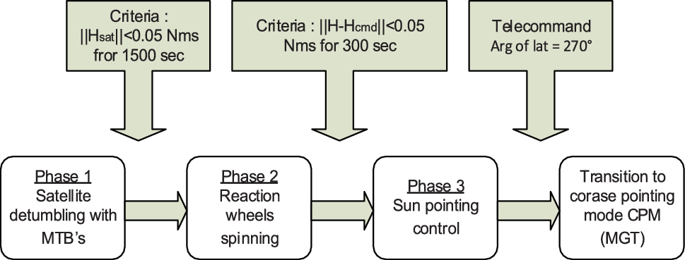
This acquisition and safe hold mode is organised into three phases, as shown in Fig. 4.

• ‐ Phase 1 (detumble submode): Just after separation from the launcher, high rates are observed due to tumbling. These high rates are reduced by magnetic damping using MTBs. The set point of the angular momentum is 0.05Nms for about 1,500s, being a criterion for the transition to the next phase.

  

  Figure 4. Initial acquisition mode phases.

The first term of the magnetic momentum $\overrightarrow {{M_{11}}\;} $ is determined from the derived Earth magnetic field $\vec B$ . The second term of the command $\overrightarrow {{M_{12}}} $ is derived from the estimated satellite angular momentum ${\vec H_{SAT}}$ such that

(1) \begin{equation}\vec M = {\vec M_{11}} + {\vec M_{12}} = - \frac{{{I_{SAT}}}}{{{\tau_{11}}{B^2}}}\overrightarrow {\dot B} + \frac{{\vec B \wedge \left( { - \frac{{{{\vec H}_{SAT}}}}{{{\tau_{12}}}}} \right)}}{{{B^2}}}\end{equation}

where $\vec M$ is the total magnetic momentum, ${\vec M_{11}}\;$ is the first term of the magnetic momentum, ${\vec M_{12}}$ is the second term of the magnetic momentum, ${I_{SAT}}$ is the satellite inertia, $\vec B$ is the Earth magnetic field, $\overrightarrow {\dot B} $ is the derived Earth magnetic field, ${\vec H_{SAT}}$ is the satellite angular momentum, ${\tau_{11}}$ is the filter time constant (first term) and ${\tau_{12}}$ is the filter time constant (second term).

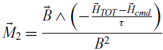
• ‐ Phase 2 (spinning submode): The wheels are switched on and spin until reaching an angular momentum along the X_sat axis with a magnitude of −0.15Nms. Here, the criterion to be satisfied to move on to the next phase is based on the difference between the total angular momentum and the commanded angular momentum, compared with a threshold of 0.05Nms during at least 300 s. In this phase, the command applied to the MTB is implemented using the equation

  (2) \begin{equation}{\vec M_2} = \frac{{\vec B \wedge \left( { - \frac{{{{\vec H}_{TOT}} - {{\vec H}_{cmd}}}}{\tau }} \right)}}{{{B^2}}}\end{equation}

where ${\vec M_2}$ is the Total magnetic momentum, ${\vec H_{cmd}}$ is the commanded angular momentum, ${\vec H_{TOT}}$ is the total angular momentum (satellite + reaction wheel angular momentum) and $\tau $ is the filter time constant

• ‐ Phase 3 (Sun acquisition submode): This is the converged phase of the mode, where the solar panels and–X_sat are pointing toward the Sun within reduced limits.

The control is achieved by two commands: the first term of the command $\overrightarrow {{M_{31}}} \;$ brings the total angular momentum to the desired set point, while the second term of the command $\overrightarrow {{M_{32}}} \;$ determines the orientation of the total angular momentum to the Sun direction:

(3) \begin{equation}{\vec M_3} = {\vec M_{31}} + {\vec M_{32}}\end{equation}

where

(4) \begin{equation}{\vec M_{31}} = \frac{{\vec B \wedge \left( { - \frac{{\left( {{{\vec H}_{TOT}} - {{\vec H}_{cmd}}} \right)}}{{{\tau_{31}}}}} \right)}}{{{B^2}}}\end{equation}

and

(5) \begin{equation}{\vec M_{32}} = \frac{{\vec B \wedge \left( {\frac{{\left[ {{{\vec H}_{TOT}} \wedge \left( {\vec S \wedge {{\vec H}_{TOT}}} \right)} \right]}}{{{\tau_{32}}{{\vec H}_{TOT}}}}} \right)}}{{{B^2}}}\end{equation}

where ${\vec M_3}$ is the total magnetic momentum, ${\vec M_{31}}$ is the first term of the magnetic momentum, ${\vec M_{32}}$ is the second term of the magnetic momentum, ${\vec H_{cmd}}$ is the commanded angular momentum, ${\vec H_{TOT}}$ is the total angular momentum (satellite + reaction wheel angular momentum), $\vec S$ is the solar direction unit vector, ${\tau_{31}}$ is the filter time constant (first term) and ${\tau_{32}}$ is the Filter time constant (second term).

2.2.2 Coarse pointing mode (MGT)

The coarse transition mode (MGT) is a control mode allowing the acquisition of correct pointing (to within a few degrees) with respect to the geocentric or heliocentric pointing command from any initial attitude. It uses magnetic measurement and control and requires knowledge of the absolute position of the satellite with sufficient precision (to calculate an adequate magnetic field command). It is a robust mode since it requires little equipment (magnetometer, magnetorquer and reaction wheels). Compared with previous microsatellites in the MYRIAD series, the special feature of ALSAT-2B is that it uses four wheels placed in a pyramidal configuration, which allows greater capacity in terms of angular momentum. The need for this transition mode is mainly linked to the stellar sensor used in MNO, which must not be dazzled at the transition to this mode. MGT is also used to converge the gyrostellar estimator under controlled conditions.

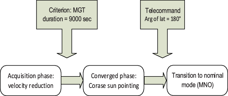
Functionally, the MGT is composed of two phases:

• • An acquisition phase, intended to reduce the satellite angular velocities and acquire rough pointing of the set point (on ALSAT-2B, the set point is heliocentric). The need for this phase is due to the change of control between the MAS and the MGT, which can cause significant disturbances in satellite speed (passage from a wheel angular momentum on X_sat to an angular momentum on Y_sat).

• • A so-called converged phase during which the heliocentric pointing is improved to enter the MGT output specifications. Figure 5 shows a schematic diagram of the MGT phases.

  

  Figure 5. MGT phases.

The principle of MGT, or compass mode, is to create a magnetic moment ${\vec M_{COM}}$ on board the satellite in the direction $\overrightarrow {{b_0}} $ that the Earth’s magnetic field would have if the satellite were well pointed. In the case where the satellite is not well pointed, a magnetic couple is created by the action of the commanded magnetic moment on the surrounding magnetic field $\vec B$ , which will naturally tend to align the vector $\overrightarrow {{b_0}} $ following $\vec B$ in the same manner that a compass needle aligns with the local magnetic field.

A term depending on the derivative of the measured magnetic field introduces damping into the control loop.

The control is then optimised by removing the component of the magnetic moment parallel to the measured field, which would in any case create no torque.

Finally, the magnetic moment is normalised with respect to the direction of the ordered moment, taking into account the maximum capacity of the MTBs.

The ${\vec M_{COM}}$ controlled magnetic moment is given by

(6) \begin{equation}\vec{M}_{0} =\frac{K\overrightarrow{\mathop{\dot{b}_{0} } }+D\left(\overrightarrow{\mathop{\dot{b}_{0} }}-\overrightarrow{\dot{b}}\right)}{\vec{B}}\end{equation}

(7) \begin{equation}\overrightarrow {{M_1}} = \overrightarrow {{M_0}} - \left( {\overrightarrow {{M_0}} \;.\;\vec b} \right).\vec b\end{equation}

(8) \begin{equation}\overrightarrow {{M_{COM}}} = \frac{{\overrightarrow {{M_1}} }}{{\max \left( {1\;,\;\left| {\frac{{{M_{1x}}}}{{{M_{max}}}}} \right|\;,\left| {\frac{{_{1y}}}{{{M_{max}}}}} \right|\;,\;\left| {\frac{{{M_{1z}}}}{{{M_{max}}}}} \right|} \right)}}\end{equation}

where $\vec b$ is the direction of the measured magnetic field vector, $\vec b = \;\frac{{\vec B}}{{\vec B}}$ , ${\vec b_0}$ is the direction of the commanded magnetic field vector, $K$ is the proportional gain (scalar), $D$ is the derived gain (matrix), and ${\vec M_{max}}$ is the maximum capacity of the MTBs.

2.2.3 Normal mode (MNO)

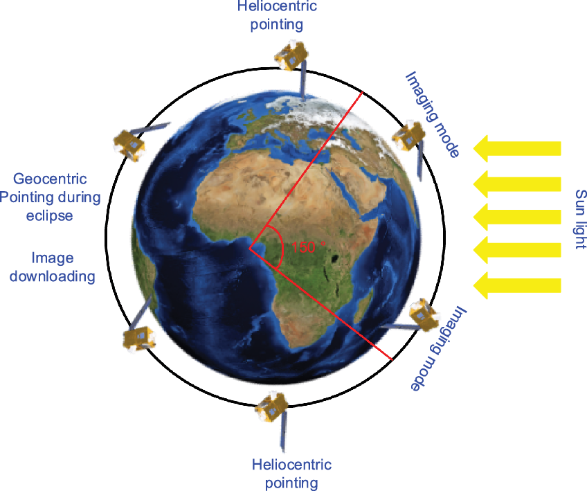
The MNO mode is the operational mode of the satellite, implementing the pointing modes required to perform imaging as well as attitude manoeuvres to achieve pointing. Attitude estimation is performed by the stellar sensor, the measurement of which is combined with that of the gyroscopes to ensure better availability of attitude measurements during the mission. Control is enabled by the four reaction wheels arranged according to an optimised pyramidal configuration, with respect to the control requirements for the three axes of the satellite, while the magnetorquers ensure the desaturation of the wheels. The attitude of the satellite in MNO is as follows:

• • Heliocentric pointing, i.e. the solar panel is pointed towards the Sun with sinusoidal motion, with rotation of $\sim$ 0.025°/s about its – X_sat axis to avoid dazzling of the star tracker (SST) by the ground at the poles.

• • Geocentric pointing in eclipse: the X_sat axis faces the Earth to allow data download.

• • Mission pointing for imaging, with respect to the local orbital reference frame, corresponding either to the manoeuvring phases during imaging missions or to the day/night or night/day maneuvers. Figure 6 illustrates the different satellite pointing modes.

  

  Figure 6. Different pointings of ALSAT-2B.

The estimation process can be split into three phases^{(Reference Ghezal, Polle, Rabejac and Montel11)} (Fig. 7):

• ‐ Prediction of the state vector: From the estimated quaternion at the previous time step and the gyro measurement, a predicted quaternion is calculated. The predicted drift is equal to the estimated drift at the previous time step.

• ‐ Innovation calculation: The angular difference between the SST-measured quaternion and the estimated quaternion is calculated at the SST measurement date, with referecen to the SST axes.

• ‐ Correction: The predicted attitude quaternion is corrected by the innovation, previously multiplied by the estimator gain.

Figure 7. ALSTA-2B gyrostellar estimator architecture.

Prediction

The prediction is based upon the following kinematics equation:

(9) \begin{equation}\dot Q = \frac{1}{2}Q \otimes \Omega \end{equation}

where $\Omega=\left[\begin{array}{c}0\\ \underline{\underline{\omega}}\end{array}\right], \underline{\omega}$ is the angular velocity rate with respect to the inertial frame, expressed in the satellite frame and $ \otimes $ is quaternion multiplication.

The equation is discretised using the Wilcox method:

(10) \begin{equation}\left\{\begin{array}{c} {\hat{Q}_{N/N-1} = \hat{Q}_{N-1/N-1} \otimes \delta Q_{N} } \\[5pt] \hat{\!d}_{N/N-1} = \ \hat{\!d}_{N-1/N-1} \end{array}\right.\end{equation}

where $\hat{Q}_{N/N}$ is the estimated attitude quaternion with respect to the inertial measurement frame at ${T_N}$ , $\hat{Q}_{N/N-1}$ is the predicted attitude quaternion with respect to the inertial measurement frame at ${T_{N - 1}}$ and $\hat{d}_{N/N-1}$ is the predicted gyro drift at ${T_N}$ , estimated at ${T_{N - 1}}$ because no gyro drift evolution model is available.

Innovation computation

The predicted quaternion defines the rotation between the inertial frame and the satellite frame (body frame), expressed in the SST measurement frame:

(11) \begin{equation}\hat{Q}_{IST} = \hat{Q}_{IB} \otimes Q_{BST}\end{equation}

The innovation is obtained through a multiplication by the SST measurement:

(12) \begin{equation}\left(\begin{array}{c} {0} \\[1pt] {\Delta \theta_{INV}} \end{array}\right)= \left(\begin{array}{c} {0} \\[5pt] {\Delta \theta_{INV,x} } \\[5pt] {\Delta \theta_{INV,y} } \\[5pt] {\Delta \theta_{INV,z} } \end{array}\right)=2 \hat{Q}_{IST} \otimes Q_{IST}^{MST}\end{equation}

where $Q_{_{}IS{T_{}}}^{MST}$ is the SST measurement, expressing the rotation between the inertial frame and the SST measurement frame and $\Delta {\theta_{INV,x}},\Delta {\theta_{INV,Y}},\Delta {\theta_{INV,z}}$ are the Euler angles of the rotation between the predicted and measured attitude of the satellite, expressed in the SST reference.

Correction

The correction vector ${X_{COR}}$ to be applied to the predicted state vector is

(13) \begin{equation}{{\bf{X}}_C} = \left( {\begin{array}{c}{\theta_C^{ST}}\\[5pt] {{d_C}}\end{array}} \right) = \left({\begin{array}{c}{\theta_{XC}^{ST}}\\[5pt] {\theta_{YC}^{ST}}\\[6pt] {\theta_{ZC}^{ST}}\\[6pt] {{d_{XC}}}\\[3pt] {{d_{YC}}}\\[3pt] {{d_{ZC}}}\end{array}} \right) = {{\bf{K}}_{KAL}}{\bf{\Delta }}{\theta_{INV}}\end{equation}

where $\theta_{XC}^{ST},\theta_{YC}^{ST},\theta_{ZC}^{ST}$ are the attitude corrections expressed in the SST measurement frame,

${d_{XC}},{d_{YC}},{d_{ZC}}$ are the drift corrections and ${{\bf{K}}_{KAL}}$ is the correction gain as a constant matrix with dimensions of 7 × 3.

The correction Euler angles are then transferred from the SST measurement frame to the satellite reference frame:

(14) \begin{equation}\theta_C^B = {Q_{BST}}\theta_C^{ST}\hat{Q}_{BST}\end{equation}

The estimated attitude at date T _N is then

(15) \begin{equation}\hat{Q}_{N/N} = \hat{Q}_{N/N-1} \otimes Q_{C,N}\end{equation}

And the estimated drift is

(16) \begin{equation} \hat{\!d}_{N/N} =\ \hat{\!d}_{N/N-1} +d_{C,N}\end{equation}

Agility performance has become one of the key factors in developing/operating modern satellite systems, especially for Earth imaging, because it determines the number of imaging targets available within the duration of a given pass.

Note here that the pyramidal configuration is one of the key features of ALSAT-2 satellites, being the first time that it has been applied on board, aimed to improve the satellite momentum to be agile and to ensure back/forward as well as along/across-track imaging (Fig. 8)^{(Reference Benzeniar and Meghabber7)}.

Figure 8. ALSAT-2B reaction wheel mounted in pyramid configuration.

The control process uses a proportional–derivative controller during the converged nominal mode:

(17) \begin{equation}{C_{com}} = - {K_p}\theta - {K_d}\dot \theta \end{equation}

where ${C_{com}}$ is the torque applied to the wheels, $\theta $ is the estimated angle from the star tracker, $\dot \theta $ is the estimated velocity from the gyroscope, ${K_p}$ is the proportional gain and ${K_d}$ is the derivative gain.

The reaction wheels generate maximum torque if two wheels rotate in one direction while the other two rotate in the opposite direction (with respect to the Y- and Z-axes).

(18) \begin{align} {C_x} & = 4 \times {C_{wheel}} \times sin\beta\nonumber \\[3pt] {C_y} & = 4 \times {C_{wheel}} \times cos\beta \times cos\alpha \\[3pt] {C_z} & = 4 \times {C_{wheel}} \times sin\alpha \times cos\beta\nonumber \end{align}

where ${C_{wheel}}$ is the elementary torque generated by a single wheel

We suppose $\vec{h}_{i}$ the angular momentum of wheel i (i = 1–4). All four wheels contribute to generate the total angular momentum of the satellite $\vec H$ :

(19) \begin{equation}{\vec H_{sat}} = \mathop \sum \limits_{ = 1}^4 \overrightarrow {{h_i}}\end{equation}

The angles α and β have values of 48° and 19° respectively, and the projection of the four h _i vectors on the X–Y–Z axes is given by the relation

(20) \begin{align}\left[ \begin{array}{c}{{H_x}}\\[4pt] {{H_y}}\\[4pt] {{H_z}}\end{array} \right] = \left[ \begin{array}{c@{\quad}c@{\quad}c@{\quad}c} - {\rm{sin}}\beta & {{\rm{sin}}\beta } & {{\rm{sin}}\beta } & { - {\rm{sin}}\beta }\\[4pt] {{\rm{cos}}\alpha {\rm{cos}}\beta } & {{\rm{cos}}\alpha {\rm{cos}}\beta } & { - {\rm{cos}}\alpha {\rm{cos}}\beta } & { - {\rm{cos}}\alpha {\rm{cos}}\beta }\\[4pt] {{\rm{cos}}\alpha {\rm{sin}}\beta } & {{\rm{cos}}\alpha {\rm{sin}}\beta } & {{\rm{cos}}\alpha {\rm{sin}}\beta } & {{\rm{cos}}\alpha {\rm{sin}}\beta }\end{array} \right] \left[ \begin{array}{c} {{h_1}}\\[4pt] {{h_2}}\\[4pt] {{h_3}}\\[4pt] {{h_4}}\end{array} \right]\end{align}

Wheel unloading or desaturation is enabled by the three magnetorquers using the following control law:

(21) \begin{equation}{\vec C_{desat}} = {K_p}\left( {{{\vec H}_{com}} - {{\vec H}_{sat}}} \right) + {K_i}\smallint \left( {{{\vec H}_{com}} - {{\vec H}_{sat}}} \right)dt\end{equation}

The magnetic moment command to the magnetorquers is then given as

(22) \begin{equation}\vec M = \frac{{{{\vec C}_{desat}} \otimes \vec B}}{{{B^2}}}\end{equation}

where ${\vec C_{desat}}$ is the desaturation torque applied to the wheels, ${\vec H_{com}}$ is the commanded angular momentum, ${\vec H_{sat}}$ is the measured satellite angular momentum, ${K_p}$ is the proportional gain, ${K_d}$ is the integral gain, $\vec M$ is the applied magnetic moment and $\vec B$ the Earth’s magnetic field.

Here, we give a brief description of the manoeuvre, but first we should distinguish between the day/night or night/day transitions and imaging manoeuvre. The former is dedicated to avoiding the star tracker being dazzled by the Earth, hence providing good performance in terms of availability. This transition manoeuvre consists of three profiles, starting with an acceleration to get a maximum torque according to

(23) \begin{equation}{\vec w_{{\rm{max}}allowed}} = \frac{{{{\vec H}_{{\rm{max}}wheel}}}}{{\mathop {{\rm{max}}\left| {{A_{wheel}}\left( i \right)} \right|}\limits_{i = 1,4} }}\end{equation}

(24) \begin{equation}{\vec H_{wheel}} = G \cdot {\vec H_{sat}} = \vec w \cdot G \cdot {I_{sat}}\end{equation}

where $\;{{{\vec{\rm w}}}_{{\rm{maxallowed}}}}$ is the maximum allowable angular velocity, $\;{{{\vec{\rm H}}}_{{\rm{wheel}}}}\,,\,{{\vec{\rm H}}_{{\rm{sat}}}}$ are the wheel and satellite angular momentum, I _sat is the satellite inertia (3 × 3 matrix), G is a 3 × 4 matrix used to extract the wheel momentum from the satellite momentum and ${\rm{\;}}{{\rm{A}}_{{\rm{wheel}}}} = {\rm{G}} \cdot {{\rm{I}}_{{\rm{sat}}}}$ (a four-dimensional vector).

Once the maximum velocity has been reached, a constant velocity is commanded, to avoid a long transient response before going to a deceleration profile. This is how the manoeuvre is implemented as shown in Figure 9.

Figure 9. Slew manoeuvre profile.

Now, for an imaging manoeuvre, we just add a settling profile (the fourth profile) to ensure perfect stability (30µrad peak to peak /4Hz) during imaging. The profile duration depends on the manoeuvre amplitude.

2.2.4 Orbit control mode (MCO)

The orbit control mode is intended to modify the orbital parameters. The off-modulation thrusters perform attitude control for the three axes. Thus, the thrusters provide both thrust, making it possible to correct the orbit, as well as attitude control. The propulsion subsystem, composed essentially of a tank sized to carry a maximum mass of 4.7kg of hydrazine, operates according to the “blow down” mode with tank pressure in the range from 24 to 5.5bar. The tank also contains the helium necessary for pressurisation. The technology used to separate the pressurising gas from the hydrazine is an impermeable elastomeric membrane. It guarantees a gas-bubble-free draw regardless of the specified environmental conditions. A thermal control function of the tank (by software) is implemented on ALSAT-2B to limit the operating pressure at the beginning of life. At the beginning of life, the thermal control of the tank ensures a temperature of 20°C, with a maximum pressure of 24bar (at 30°C). Four 1N thrusters, each fitted with two solenoid valves in series, are controlled by the power control and distribution unit (PCDU) to apply thrust. The thrusters can operate in continuous or pulsed mode. Figure 10(a) illustrates the ALSAT-2B propulsion subsystem architecture, while Fig. 10(b) shows the design implemented for the propulsion subsystem.

Figure 10. (a) ALSAT-2B propulsion subsystem architecture. (b) ALSAT-2B propulsion subsystem design.

The exit from the MCO mode is managed automatically. When the total number of pulses produced by the four thrusters reaches the requested value, it returns to MNO mode. Before the thrust execution, the ground programs one heliocentric orbit pointing, and after the thrust, two more heliocentric orbits are carried out to recharge the batteries and converge the payload thermal control. We distinguish three types of rallies towards the thrust attitude:

• ‐ A slew manoeuvre along the pitch axis for in-plane orbit correction (alignment of the thrust direction with the velocity vector)

• ‐ A slew manoeuvre along the roll axis for out-of-plane orbit correction (alignment of the thrust direction normal to the orbit plane)

• ‐ A combined roll/pitch slew manoeuvre, bringing the satellite X_sat axis into the plane containing the velocity vector and the normal to the orbit, which makes it possible to carry out a combined correction of the semi-major axis and the inclination. Optimal efficiency is obtained when the satellite X_sat axis is located at 45° from the velocity vector and from the normal to the orbit. The attitude measurement comes from the three gyroscopes; this allows these manoeuvres to be performed at any orbital position, since measurements are available continuosuly from the gyroscopes (with no need for a solar/stellar measurement), but in return this requires initialisation of this measurement. The estimator initialisation is performed at the beginning of the MCO mode using the estimate provided from the MNO mode.