2.1 Problem definition

To examine the near-tip behaviour of a fluid-driven fracture, we consider the problem of a semi-infinite fracture (figure 1) propagating with constant velocity $V$, which is understood as the instantaneous local tip velocity of the parent hydraulic fracture (HF). The host permeable linear-elastic rock is characterised by Young’s modulus $E$ and Poisson’s ratio $\unicode[STIX]{x1D708}$. Small-scale yielding (Rice Reference Rice and Liebowitz1968), i.e. it is assumed that the rock damage/yielding zone at the advancing fracture front is small compared to the length scales of other physical processes active near the tip (e.g. dissipation in the viscous fluid flow). Linear elastic fracture mechanics (LEFM) theory is therefore utilised for the modelling of the quasi-static propagation of the fracture in the rock characterised by the fracture toughness $K_{Ic}$.

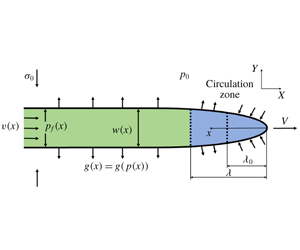
In figure 1 we show the schematics of the considered problem. The fracture, loaded internally by the fluid pressure $p_{f}(x)$, opens (with aperture distribution $w(x)$) against the in situ confining stress $\unicode[STIX]{x1D70E}_{o}$. We consider fluids presented in the model as Newtonian. Fluid flow in the fracture is described by lubrication theory (Batchelor Reference Batchelor1967).

Figure 1. Schematic picture of the fracture tip model with the pressure-dependent fluid exchange between the fracture and permeable saturated rock.

The rock adjacent to the fracture is permeable and saturated by pore fluid at ambient pore pressure $p_{o}$. The fluid exchange between the fracture and the reservoir is driven by the pressure difference between the fracture ($p_{f}$) and the reservoir ($p_{o}$). The fluid exchange process is modelled by one-dimensional pressure-dependent leak-off/leak-in (PDL) driven by pore pressure diffusion in the rock (Detournay & Garagash Reference Detournay and Garagash2003; Kovalyshen Reference Kovalyshen2010; Kovalyshen & Detournay Reference Kovalyshen and Detournay2013). This model is a convenient approximation of a full two-dimensional leak-off and associated diffusion problem (Detournay & Garagash Reference Detournay and Garagash2003) based on the assumption that the characteristic thickness of the diffusive boundary layer around the crack is small compared to the characteristic length scale of the fracture tip problem. The local rate of the fluid exchange is denoted by $g(x)$. We also assume that the pore and hydraulic fracturing fluids have similar (identical in the model) properties.

Fluid pressure $p_{f}(x)$ diminishes in the fluid flow along the fracture towards the tip. If its value at the tip, $p_{f}(0)$, drops below $p_{o}$, there exists a near-tip zone of some length $\unicode[STIX]{x1D706}_{o}$ ($x\in [0,\unicode[STIX]{x1D706}_{o}]$) along which the pore fluid flows into the fracture from the surrounding rock. For distances larger than $\unicode[STIX]{x1D706}_{o}$, the fluid pressure recovers enough to enable the leak-off of the formation fluid from the fracture back into the rock. Owing to the steady crack propagation (i.e. problem is stationary in the coordinate system $x$ moving with the crack tip), all of the formation fluid leaked-in along $x\in [0,\unicode[STIX]{x1D706}_{o}]$ has to circulate (leak-off) back into the formation, thus defining the pore-fluid circulation zone of some length $\unicode[STIX]{x1D706}>\unicode[STIX]{x1D706}_{o}$ near the fracture tip (figure 1). The crack channel within the interval $[\unicode[STIX]{x1D706},+\infty )$ is filled by the hydraulic fracturing fluid which, due to pressure continuity, is also expected to leak-off into the rock.

2.2 Governing equations

Let us consider the moving coordinate system ($x,y$) related to the fixed coordinate system ($X,Y$) by equations: $x=Vt-X$ and $y=Y$. The considered problem is stationary in the moving coordinate system. The governing equations are written for unknown fracture opening $w(x)$ and net pressure distribution $p(x)=p_{f}(x)-\unicode[STIX]{x1D70E}_{o}$ along the fracture ($0<x<+\infty$), elaborating further on the framework proposed by Garagash et al. (Reference Garagash, Detournay and Adachi2011).

2.2.1 Fracture propagation

Linear elastic fracture mechanics fracture propagation criteria under quasi-static conditions states that the stress intensity factor at the crack tip matches the rock toughness: $K_{I}=K_{Ic}$. This condition prescribes the asymptotic behaviour of the fracture opening near its front (Irwin Reference Irwin1957):

(2.1)$$\begin{eqnarray}w(x)=\frac{K^{\prime }}{E^{\prime }}\sqrt{x}.\end{eqnarray}$$

Here $E^{\prime }=E/(1-\unicode[STIX]{x1D708}^{2})$ is the plane strain modulus and $K^{\prime }=4\sqrt{(2/\unicode[STIX]{x03C0})}K_{Ic}$ is the toughness parameter.

2.2.2 Crack elasticity

The net pressure $p(x)$ in the fracture can be expressed as the crack line integral of the opening $w(x)$ using the elasticity equation (Bilby & Eshelby Reference Bilby, Eshelby and Liebowitz1968)

(2.2)$$\begin{eqnarray}p(x)=\frac{E^{\prime }}{4\unicode[STIX]{x03C0}}\int _{0}^{\infty }\frac{\text{d}w(s)}{\text{d}s}\frac{\text{d}s}{x-s}.\end{eqnarray}$$

Equation (2.2) can be inverted (Garagash & Detournay Reference Garagash and Detournay2000) to aid in the numerical implementation of the problem solution, i.e.

(2.3)$$\begin{eqnarray}w(x)=\frac{K^{\prime }}{E^{\prime }}\sqrt{x}+\frac{4}{\unicode[STIX]{x03C0}E^{\prime }}\int _{0}^{\infty }K(x,s)p(s)\,\text{d}s,\end{eqnarray}$$

where the integral kernel is $K(x,s)=\ln |(\sqrt{x}+\sqrt{s})/(\sqrt{x}-\sqrt{s})|-2\sqrt{x/s}$. This form of crack elasticity equation already accounts for the propagation condition (2.1) (i.e. the integral in (2.3) is $o(\sqrt{x})$).

2.2.3 Fluid flow

The flow of a viscous incompressible fluid in the crack channel is described by the continuity equation averaged across the fracture aperture, which, upon transforming to the moving coordinate system, is given by

(2.4)$$\begin{eqnarray}V\frac{\text{d}w}{\text{d}x}-\frac{\text{d}(wv)}{\text{d}x}+g=0,\end{eqnarray}$$

where $g$ is the local rate of fluid exchange between the fracture and the rock ($g>0$ for leak-off and $g<0$ for leak-in) given in the PDL model by the following expression (appendix A):

(2.5)$$\begin{eqnarray}g(x)=Q^{\prime }\sqrt{V}\left(\frac{p(0)+\unicode[STIX]{x1D70E}_{o}^{\prime }}{2\sqrt{x}}+\int _{0}^{x}\frac{\text{d}p}{\text{d}x^{\prime }}\frac{\text{d}x^{\prime }}{2\sqrt{x-x^{\prime }}}\right).\end{eqnarray}$$

Here $Q^{\prime }=4k/(\unicode[STIX]{x1D707}\sqrt{\unicode[STIX]{x03C0}c})$ is a leak-in coefficient defined in terms of the pore pressure diffusivity coefficient $c$, reservoir permeability $k$ and fluid viscosity $\unicode[STIX]{x1D707}$, $p(0)=p_{f}(0)-\unicode[STIX]{x1D70E}_{o}$ is the net fluid pressure value at the fracture front, and $\unicode[STIX]{x1D70E}_{o}^{\prime }=\unicode[STIX]{x1D70E}_{o}-p_{o}$ is the ambient value of the effective confining stress.

Integrating (2.4) from the tip $x=0$ to some distance $x>0$, we obtain

(2.6a,b)$$\begin{eqnarray}wv=wV+q_{\bot },\quad q_{\bot }=\int _{0}^{x}g(s)\,\text{d}s,\end{eqnarray}$$

which signifies that the local fluid volumetric flow rate at distance $x$ from the fracture tip $w(x)v(x)$ is partitioned between the fluid stored in the fracture $w(x)V$ and in the rock via the cumulative rate of fluid exchange $q_{\bot }(x)$, given by

(2.7)$$\begin{eqnarray}q_{\bot }(x)=Q^{\prime }\sqrt{V}\int _{0}^{x}\frac{p(s)+\unicode[STIX]{x1D70E}_{o}^{\prime }}{2\sqrt{x-s}}\,\text{d}s=C^{\prime }\sqrt{Vx}+Q^{\prime }\sqrt{V}\int _{0}^{x}\frac{p(s)}{2\sqrt{x-s}}\,\text{d}s.\end{eqnarray}$$

Here $C^{\prime }=Q^{\prime }\unicode[STIX]{x1D70E}_{o}^{\prime }=4k\unicode[STIX]{x1D70E}_{o}^{\prime }/(\unicode[STIX]{x1D707}\sqrt{\unicode[STIX]{x03C0}c})$ is the Carter’s leak-off coefficient. The first term on the right-hand side of (2.7) corresponds to the classical Carter’s leak-off expression strictly valid only when $p_{f}(x)=\unicode[STIX]{x1D70E}_{o}$ (or $p(x)=0$), while the second term is the pressure-dependent correction. Since the net fluid pressure $p(x)<0$ (or $p_{f}(x)<\unicode[STIX]{x1D70E}_{o}$) in a semi-infinite hydraulic fracture (e.g. Garagash & Detournay Reference Garagash and Detournay2000), the corrective pressure-dependent term is always negative or, in other words, corresponds to a corrective leak-in.

Finally, Poiseuille’s law for the fluid velocity along the crack channel

(2.8)$$\begin{eqnarray}v=\frac{w^{2}}{\unicode[STIX]{x1D707}^{\prime }}\frac{\text{d}p}{\text{d}x},\end{eqnarray}$$

with $\unicode[STIX]{x1D707}^{\prime }=12\unicode[STIX]{x1D707}$ designating the viscosity parameter, completes the fluid flow description.

3.1 Vertex solutions

Two different mechanisms govern the propagation regime of a finite hydraulic fracture (e.g. Garagash et al. Reference Garagash, Detournay and Adachi2011). The first one is the partitioning of the injected fluid between the fracture and the reservoir as a result of the leak-in and leak-off processes (fracture storage versus fluid exchange with the rock). The second mechanism is the partitioning of the total dissipated energy between the creation of the new fracture surfaces and flow of the viscous fluid along the fracture (toughness versus viscosity).

In the process of fracture growth, the partition of the fracturing fluid and the partition of the dissipated energy change over time, which can lead to the realisation of different limiting regimes dominated by one storage mechanism and one dissipation mechanism at different times. In the context of a semi-infinite hydraulic fracture, the change in the partitioning of the fluid and energy with time can be recast into the change with the distance from the fracture tip.

One can suggest four limiting propagation regimes that are characterised by the dominance of one storage/exchange mechanism and one dissipation mechanism: toughness dominated $(\unicode[STIX]{x1D707}^{\prime }=0)$, storage-viscosity dominated $(C^{\prime }=Q^{\prime }=0,K^{\prime }=0)$, leak-off-viscosity dominated $(C^{\prime }\rightarrow \infty ,K^{\prime }=0)$ and storage-leak-in-viscosity dominated $(K^{\prime }=0,C^{\prime }>0,Q^{\prime }<+\infty )$. The corresponding solutions are referred to as ‘vertex’ solutions in a problem parametric space.

While the leak-in ($Q^{\prime }$) and the leak-off ($C^{\prime }$) coefficients define the partitioning of the fluid, viscosity $\unicode[STIX]{x1D707}^{\prime }$ and toughness $K^{\prime }$ parameters are responsible for the partitioning of the dissipated energy.

The first three vertex solutions ($k$, $m$, $\widetilde{m}$) are given, e.g. by Garagash et al. (Reference Garagash, Detournay and Adachi2011), and summarised in table 1 for completeness, in terms of the following three characteristic length scales:

(3.1a-c)$$\begin{eqnarray}\displaystyle \ell _{k}=\left(\frac{K^{\prime }}{E^{\prime }}\right)^{2},\quad \ell _{m}=V\frac{\unicode[STIX]{x1D707}^{\prime }}{E^{\prime }},\quad \ell _{\widetilde{m}}=\left(C^{\prime }\sqrt{V}\frac{\unicode[STIX]{x1D707}^{\prime }}{E^{\prime }}\right)^{2/3}. & & \displaystyle\end{eqnarray}$$

Table 1. Three limiting solutions of a semi-infinite hydraulic fracture for the identified limiting values of problem parameters.

The pressure dependency of the fluid exchange between the fracture and the rock is coupled with the fluid pressure drop in the flow toward the crack tip (when viscosity is non-negligible: $\unicode[STIX]{x1D707}^{\prime }>0$). This fact suggests that the leak-in dominates near the fracture front. In other words, we anticipate that in the vicinity of the fracture tip the newly created crack volume (storage) is accommodated entirely by the pore fluid leaking-in from the rock (while the fluid flow towards the fracture tip along the crack channel is negligible there, $v\approx 0$). However, this dominance of the leak-in has to be limited to a finite near-tip region, since crack elasticity requires that $p(x)$ vanishes as $x\rightarrow \infty$, or $p_{f}(x)\rightarrow \unicode[STIX]{x1D70E}_{o}>p_{o}$, thus, eventually giving a way to the leak-off process.

Vertices $k$, $m$, $\widetilde{m}$ (table 1) are the solutions for the entire semi-infinite fracture for the corresponding limiting values of governing parameters. They can be determined from the monomial solution to the crack elasticity equation (2.2):

$$\begin{eqnarray}w_{\unicode[STIX]{x1D706}}(x)=Bx^{\unicode[STIX]{x1D706}};\quad p_{\unicode[STIX]{x1D706}}(x)=E^{\prime }Bf(\unicode[STIX]{x1D706})x^{\unicode[STIX]{x1D706}-1},\quad f(\unicode[STIX]{x1D706})=\frac{\unicode[STIX]{x1D706}\cot (\unicode[STIX]{x03C0}\unicode[STIX]{x1D706})}{4},\quad 0<\unicode[STIX]{x1D706}<1.\end{eqnarray}$$

Here particular values of the prefactor $B$ and the exponent $\unicode[STIX]{x1D706}$ are constrained by the lubrication equation when setting parameters ($C^{\prime }$, $\unicode[STIX]{x1D707}^{\prime }$ and $K^{\prime }$) to the corresponding limiting values, as detailed by Garagash et al. (Reference Garagash, Detournay and Adachi2011). In the $k$-vertex, viscosity is negligible ($\unicode[STIX]{x1D707}^{\prime }=0$) and the solution follows from the propagation condition (2.1). In the $m$-vertex, the fluid exchange ($C^{\prime }=Q^{\prime }=0$) and toughness ($K^{\prime }=0$) are negligible, and the solution is recovered by balancing the fluid flux in the crack $w(x)v(x)$ with the storage term $w(x)V$ in the continuity equation. We anticipate that in the general parametric case (i.e. not limited to the stated values of $K^{\prime }$ and other parameters) the $m$-vertex solution provides the far-field solution asymptote (e.g. Garagash et al. Reference Garagash, Detournay and Adachi2011). In the $\widetilde{m}$-vertex, the fluid storage ($C^{\prime }\rightarrow \infty$) and toughness ($K^{\prime }=0$) are negligible. In this case, the fluid flux in the crack is balanced with the Carter’s leak-off term. In the general case, the $\widetilde{m}$-vertex can be realised as an intermediate field solution (Garagash et al. Reference Garagash, Detournay and Adachi2011).

The new storage-leak-in-viscosity vertex $\widetilde{o}$ emerges as a particular case of the viscosity-dominated ($K^{\prime }=0$) behaviour linked to the dominance of the fluid leak-in (rather than the leak-off) in the near field ($x\rightarrow 0$). It corresponds to the classical zero-toughness behaviour of the crack opening, $w=B_{\widetilde{o}}x^{3/2}$, and the non-singular pressure $p=-\unicode[STIX]{x1D70E}_{0}^{\prime }-\frac{3}{2}B_{\widetilde{o}}(V^{1/2}/Q^{\prime })x$. The first term in the expression for the net pressure is obtained from balancing the leak-in and leak-off terms in the continuity equation. On the other hand, the second term arises from matching the leak-in and the fracture storage terms and gains particular importance in/near the zero-leak-off limit ($\unicode[STIX]{x1D70E}_{0}^{\prime }=0$). This vertex solution contains prefactor $B_{\widetilde{o}}$ (with units $1/\sqrt{m}$) that is unknown and a part of the overall solution. This betrays the fact that the $\widetilde{o}$-asymptote can be realised only as a near or intermediate field of the fracture, as it can not satisfy the elasticity equation over the full semi-infinite crack extent. The second term in the net pressure is found with the assumption that the $\widetilde{o}$-vertex solution is realised in the near field, and in this case, the left-hand side of the continuity equation (${\sim}w^{3}(x)p^{\prime }(x)$) for this vertex solution is negligible as compared to the terms on the right-hand side (storage, leak-off and leak-in).

For non-zero fracture toughness $K^{\prime }>0$, the near-field ($x\rightarrow 0$) behaviour of the fracture opening is given by the $k$-vertex solution (table 1), as stems from the propagation condition (2.1). The corresponding asymptotic expression for the net pressure $p(x\rightarrow 0)=-\unicode[STIX]{x1D70E}_{0}^{\prime }-(K^{\prime }V^{1/2})/(E^{\prime }Q^{\prime })$ follows from the fluid continuity equation (2.6) by balancing the fluid exchange (the leak-in pore fluid volume) with the fracture storage. (We note that the fluid flux along the crack $wv$ is negligibly small in the near-field fluid balance.) The obtained finite net pressure value at the fracture tip is drastically different from the one in the Carter’s, pressure-independent leak-off model (Garagash et al. Reference Garagash, Detournay and Adachi2011), where the pressure sustains a negative singularity as the fracturing fluid is assumed to reach the tip of the fracture. When reformulated in terms of the fluid pressure, $p_{f}(x\rightarrow 0)=p_{0}-K^{\prime }\sqrt{V}/(E^{\prime }Q^{\prime })$, this asymptote suggests that the fluid pressure at the crack tip is reduced from its drained value given by the ambient pore pressure $p_{0}$ by the amount $K^{\prime }\sqrt{V}/(E^{\prime }Q^{\prime })$. The latter, undrained pressure change vanishes for slowly propagating cracks ($V\rightarrow 0$) or/and zero rock toughness ($K^{\prime }\rightarrow 0$).

The obtained near-field $k$ ($K^{\prime }>0$) and $\widetilde{o}$ ($K^{\prime }=0$) asymptotes are summarised in table 2.

Figure 2. Parametric diagram (pyramid $m\widetilde{m}\widetilde{o}k$) and corresponding four limiting faces corresponding to the dominance of one energy dissipation or one fluid storage mechanism. Few solution trajectories parameterised by the leak-off $\unicode[STIX]{x1D712}$ and leak-in $\unicode[STIX]{x1D701}$ numbers (or their ratio $\unicode[STIX]{x1D713}=\unicode[STIX]{x1D712}/\unicode[STIX]{x1D701}$) are also shown.

Table 2. Near-field ($x\rightarrow 0$) of semi-infinite hydraulic fracture.

3.2 Structure of solution and scaling

The general solution of the considered problem can be tracked within the parametric triangular pyramid $m\widetilde{m}\widetilde{o}k$ formed by the four aforesaid vertices. The schematic diagram of this pyramid is represented in figure 2.

Four triangular faces of pyramid $m\widetilde{m}\widetilde{o}k$ correspond to either the dominance of one of the three fluid storage/exchange mechanisms or one of the dissipation mechanisms:

1. (i) storage-leak-off face $m\widetilde{m}k$: leak-in process is negligible, $Q^{\prime }=0$;

2. (ii) storage-leak-in face $m\widetilde{o}k$: leak-off process is negligible, $C^{\prime }\propto \unicode[STIX]{x1D70E}_{o}^{\prime }=0$;

3. (iii) leak-face $\widetilde{m}\widetilde{o}k$: fluid storage in the fracture is negligible, $C^{\prime }\rightarrow \infty$; and

4. (iv) viscosity-face $m\widetilde{m}\widetilde{o}$: toughness is negligible, $K^{\prime }=0$.

Six edges of the pyramid $m\widetilde{m}\widetilde{o}k$ correspond to the intersection of the corresponding two faces and, thus, reflect the dominance of one of the three fluid storage/exchange mechanisms and one of the dissipation mechanisms. For example, $\widetilde{m}\widetilde{o}$ is the leak-viscosity edge ($C^{\prime }\rightarrow \infty$ and $K^{\prime }=0$), bounding the leak $\widetilde{m}\widetilde{o}k$ ($C^{\prime }\rightarrow \infty$) and the viscosity $m\widetilde{m}\widetilde{o}$ ($K^{\prime }=0$) faces, and, thus, corresponds to the negligible storage and toughness.

The proposed pyramidal parametric space $m\widetilde{m}\widetilde{o}k$ for the fracture tip with the pressure-dependent leak-off is a direct generalisation of the triangular parametric space, face $m\widetilde{m}k$, for Carter’s (pressure-independent) leak-off (Garagash et al. Reference Garagash, Detournay and Adachi2011), by the addition of the new vertex $\widetilde{o}$. The emergent edges $\widetilde{o}k$, $\widetilde{m}\widetilde{o}$ and $m\widetilde{o}$ are expected to describe the transitions of the corresponding limiting solutions with distance from the crack tip between the corresponding vertices (from the second to the first, i.e. $\widetilde{m}\widetilde{o}$-edge corresponds to the transition from the near field $\widetilde{o}$ to the far field $\widetilde{m}$, etc). As discussed above, the $\widetilde{o}$-vertex solution can be realised only in the near field of a semi-infinite fracture, thus suggesting that the $\widetilde{o}k$-edge may in fact correspond to the near-field expansion of the $k$-vertex ($w\propto x^{1/2}$) which includes the next order correction given by the $\widetilde{o}$-vertex solution ($w\propto x^{3/2}$), and this correction may come to eventually dominate (over the $k$-term) with increasing distance from the tip.

In the case of the other two edges involving the $\widetilde{o}$-vertex as the fracture near field, i.e. $\widetilde{m}\widetilde{o}$ ($K^{\prime }=0$, $C^{\prime }\rightarrow \infty$) and $m\widetilde{o}$ ($K^{\prime }=0$, $C^{\prime }\propto \unicode[STIX]{x1D70E}_{o}^{\prime }=0$), they should in principle provide solutions for the entire semi-infinite HF under the corresponding limiting values of the parameters. Before attempting these (and other edge) solutions, let us attempt to constrain the a priori unknown near-field coefficient $B_{\widetilde{o}}$ in the $\widetilde{o}$ expression for the opening $w=B_{\widetilde{o}}x^{3/2}$ ($x\rightarrow 0$). Using the inverted form of the elasticity equation (2.3) with $K^{\prime }=0$, and formally passing to the asymptotic limit $x\rightarrow 0$ under the integral, we obtain

(3.2)$$\begin{eqnarray}B_{\widetilde{o}}=\frac{8}{3\unicode[STIX]{x03C0}E^{\prime }}\int _{0}^{\infty }\frac{p(s)}{s^{3/2}}\,\text{d}s.\end{eqnarray}$$

Since $p(s\rightarrow 0)=-\unicode[STIX]{x1D70E}_{0}^{\prime }-\frac{3}{2}B_{\widetilde{o}}(V^{1/2}/Q^{\prime })s$ (table 2), the above integral expression for $B_{\widetilde{o}}$ converges (finite) for the $m\widetilde{o}$-edge (when $\unicode[STIX]{x1D70E}_{o}^{\prime }=0$) and diverges for the $\widetilde{m}\widetilde{o}$-edge. This suggests that the underlining formal limit-taking procedure to arrive to (3.2) is not applicable to the latter ($\widetilde{m}\widetilde{o}$-edge), while conversely (3.2) can be used to constrain coefficient $B_{\widetilde{o}}$ in the former case ($m\widetilde{o}$-edge). Specifically, we observe for the $m\widetilde{o}$-edge that if the net pressure is negative in the entire crack coordinate domain ($p(s)<0$ for all $s>0$), which is suggested by the negative net pressure values in both the near field and far field, then (3.2) results in $B_{\widetilde{o}}<0$ or, in other words, negative crack opening near the tip. This contradiction rules out the existence of the $m\widetilde{o}$-edge solution (under the plausible assumption of the negative net pressure in the crack), which implies that the general solution to the problem does not have a well-defined limiting solution when both toughness and leak-off (or, conversely, ambient effective stress) equal zero.

The general solution of the fracture tip problem within the parametric pyramid transitions with increasing distance from the tip from the near-field $k$ to the far-field $m$-vertex, and in different limiting cases can collapse onto or be attracted to the series of faces and/or edges, as apparent from their parametric definitions. To identify non-dimensional parameters which fix a given solution trajectory in the parametric space, we follow the methodology of Garagash et al. (Reference Garagash, Detournay and Adachi2011) and introduce characteristic scales for the transition distance $\ell _{\ast }$, opening $w_{\ast }$ and pressure $p_{\ast }$ closely related to the evolution of the solution along a given edge in the parametric space between the two corresponding vertices, or the ‘edge scalings’.

Edge scalings $mk$, $\widetilde{m}k$ and $m\widetilde{m}$ are defined after Garagash et al. (Reference Garagash, Detournay and Adachi2011) such that the solutions for either $p(x)$ or $w(x)$ for the corresponding two vertices forming the edge in question ‘intersect’ at $x\sim \ell _{\ast }$. For example, in the case of the storage $mk$-edge, we find the characteristic length by contrasting the $k$ and $m$ asymptotes for the opening, $w_{\ast }=\ell _{k}^{1/2}\ell _{\ast }^{1/2}=\ell _{m}^{1/3}\ell _{\ast }^{2/3}$, while $p_{\ast }$ follows from the elastic scaling constraint $w_{\ast }/\ell _{\ast }=p_{\ast }/E^{\prime }$. Edge scalings which involve vertex $\widetilde{o}$ (i.e. $\widetilde{m}\widetilde{o}$ and $\widetilde{o}k$) are obtained similarly but also recognising that the $\widetilde{o}$-asymptote depends on the solution trajectory (via a priori unknown prefactor). In the $\widetilde{m}\widetilde{o}$-case the transition length scale $\ell _{\ast }$ is found by contrasting the leading order $\widetilde{o}$-asymptote for the net pressure (i.e. $p\approx -\unicode[STIX]{x1D70E}_{o}^{\prime }$) with that of the $\widetilde{m}$-vertex, i.e. $p_{\ast }=\unicode[STIX]{x1D70E}_{o}^{\prime }=E^{\prime }(\ell _{\widetilde{m}}/\ell _{\ast })^{3/8}$, while $w_{\ast }$ follows from the elastic constraint. In the $\widetilde{o}k$-scaling the characteristic pressure is taken equal to $p_{\ast }=\unicode[STIX]{x1D70E}_{0}^{\prime }$. Using $p_{\ast }$, elastic scaling constraint and balancing $\widetilde{o}$- and $k$-vertex solutions, we find that $\ell _{\ast }=K^{\prime 2}/\unicode[STIX]{x1D70E}_{o}^{\prime 2}$ and $w_{\ast }=K^{\prime 2}/E^{\prime }\unicode[STIX]{x1D70E}_{o}^{\prime }$. All of the above edge scalings are recorded in table 3.

Table 3. Characteristic distance from the tip $\ell _{\ast }$, pressure $p_{\ast }$ and opening $w_{\ast }=(p_{\ast }/E^{\prime })\ell _{\ast }$, corresponding to the five scalings of the problem.

Comparing three transition (edge) length scales within a given parametric face of the pyramid $m\widetilde{m}\widetilde{o}k$ allows us to identify a ‘trajectory number’ parameterising that face solution. Considering, for example, the zero-leak-in face $m\widetilde{m}k$, one can introduce a single number expressible as a ratio of any two of the face’s three transition length scales ($\ell _{mk}$, $\ell _{m\widetilde{m}}$, and $\ell _{\widetilde{m}k}$) (Garagash et al. Reference Garagash, Detournay and Adachi2011):

(3.3)$$\begin{eqnarray}\unicode[STIX]{x1D712}=\left(\frac{\ell _{m\widetilde{m}}}{\ell _{mk}}\right)^{1/6}=\left(\frac{\ell _{mk}}{\ell _{\widetilde{m}k}}\right)^{1/2}=\left(\frac{\ell _{m\widetilde{m}}}{\ell _{\widetilde{m}k}}\right)^{1/8}=\frac{C^{\prime }E^{\prime }}{K^{\prime }V^{1/2}}.\end{eqnarray}$$

This number, which can be interpreted as a dimensionless leak-off or ambient effective stress (since $C^{\prime }=Q^{\prime }\unicode[STIX]{x1D70E}_{o}^{\prime }$), or non-dimensional reciprocal of toughness, parameterises solution trajectory within the $m\widetilde{m}k$-face. The limiting case $\unicode[STIX]{x1D712}\rightarrow 0$ corresponds to the storage-dominated $mk$-edge solution

(3.4)$$\begin{eqnarray}\text{zero leak-in},\quad \unicode[STIX]{x1D712}=0:\quad k\underset{\ell _{mk}}{\rightarrow }m,\end{eqnarray}$$

which transitions from the $k$- to the $m$-vertex with distance from the tip over length scale $\ell _{mk}$ (shown by the blue coloured trajectory in figure 2). While the other limiting case $\unicode[STIX]{x1D712}\rightarrow \infty$ corresponds to the separation of the corresponding transitional scales, $\ell _{\widetilde{m}k}\ll \ell _{m\widetilde{m}}$, (3.3), leading to the nested solution structure corresponding to the succession of the two edge solutions ($\widetilde{m}k$ and $m\widetilde{m}$)

(3.5)$$\begin{eqnarray}\text{zero leak-in},\quad \unicode[STIX]{x1D712}\rightarrow \infty :\quad k\underset{\ell _{\widetilde{m}k}}{\rightarrow }\widetilde{m}\underset{\ell _{m\widetilde{m}}}{\rightarrow }m,\end{eqnarray}$$

signifying transition with distance from the tip first from the $k$- to $\widetilde{m}$-vertex over length scale $\ell _{\widetilde{m}k}$ and then from the $\widetilde{m}$- to $m$-vertex over length scale $\ell _{m\widetilde{m}}$ (shown by the brown coloured trajectory in figure 2).

Similarly, for the zero-storage face $\widetilde{m}\widetilde{o}k$, $\unicode[STIX]{x1D712}\rightarrow \infty$, we define another number in terms of the ratios of any two of the corresponding three edge length scales ($\ell _{\widetilde{o}k}$, $\ell _{\widetilde{m}\widetilde{o}}$, and $\ell _{\widetilde{m}k}$)

(3.6)$$\begin{eqnarray}\unicode[STIX]{x1D701}=\left(\frac{\ell _{\widetilde{o}k}}{\ell _{\widetilde{m}k}}\right)^{1/6}=\left(\frac{\ell _{\widetilde{m}\widetilde{o}}}{\ell _{\widetilde{o}k}}\right)^{1/2}=\left(\frac{\ell _{\widetilde{m}\widetilde{o}}}{\ell _{\widetilde{m}k}}\right)^{1/8}=\frac{E^{\prime }}{K^{\prime }}\left(\unicode[STIX]{x1D707}^{\prime }Q^{\prime }V^{1/2}\right)^{1/3},\end{eqnarray}$$

which can be interpreted as dimensionless leak-in or a reciprocal of toughness. This number parameterises solution trajectory within the $\widetilde{m}\widetilde{o}k$-face. The limiting case $\unicode[STIX]{x1D701}\rightarrow 0$ corresponds to the leak-off-dominated $\widetilde{m}k$-edge solution, also a part of the limiting trajectory (3.5) in the $m\widetilde{m}k$-face. While $\unicode[STIX]{x1D701}\rightarrow \infty$ corresponds to the separation of the relevant transitional scales, $\ell _{\widetilde{o}k}\ll \ell _{\widetilde{m}\widetilde{o}}$, (3.6), leading to the nested solution structure corresponding to the succession of the two edge solutions ($\widetilde{o}k$ and $\widetilde{m}\widetilde{o}$) with distance from the tip

(3.7)$$\begin{eqnarray}\unicode[STIX]{x1D712}\rightarrow \infty ,\quad \unicode[STIX]{x1D701}\rightarrow \infty :\quad k\underset{\ell _{\widetilde{o}k}}{\rightarrow }\widetilde{o}\underset{\ell _{\widetilde{m}\widetilde{o}}}{\rightarrow }\widetilde{m}.\end{eqnarray}$$

For the zero-toughness face $m\widetilde{m}\widetilde{o}$, $\unicode[STIX]{x1D712}\rightarrow \infty$, we can define another number in terms of the ratio of the $\widetilde{m}\widetilde{o}$- and $m\widetilde{m}$-edge length scales

(3.8)$$\begin{eqnarray}\unicode[STIX]{x1D713}=\left(\frac{\ell _{m\widetilde{m}}}{\ell _{\widetilde{m}\widetilde{o}}}\right)^{1/8}=\unicode[STIX]{x1D70E}_{o}^{\prime }\left(\frac{Q^{\prime }}{\unicode[STIX]{x1D707}^{\prime 1/2}V}\right)^{2/3},\end{eqnarray}$$

which can be interpreted as, e.g. a dimensionless effective confining stress. Note that $\unicode[STIX]{x1D713}$ is not an independent parameter, but expressible in terms of the previously introduced leak-off $\unicode[STIX]{x1D712}$ and leak-in $\unicode[STIX]{x1D701}$ numbers, $\unicode[STIX]{x1D713}=\unicode[STIX]{x1D712}/\unicode[STIX]{x1D701}$. This number parameterises solution trajectory within the $m\widetilde{m}\widetilde{o}$-face, such that $\unicode[STIX]{x1D713}\rightarrow \infty$ corresponds to the separation of the two length scales, $\ell _{\widetilde{m}\widetilde{o}}\ll \ell _{m\widetilde{m}}$, (3.8), resulting in a solution comprised of the two edge solutions ($m\widetilde{o}$ and $m\widetilde{m}$)

(3.9)$$\begin{eqnarray}\unicode[STIX]{x1D712}\rightarrow \infty ,\quad \unicode[STIX]{x1D713}=\unicode[STIX]{x1D712}/\unicode[STIX]{x1D701}\rightarrow \infty :\quad \widetilde{o}\underset{\ell _{\widetilde{m}\widetilde{o}}}{\rightarrow }\widetilde{m}\underset{\ell _{m\widetilde{m}}}{\rightarrow }m.\end{eqnarray}$$

The other limit, $\unicode[STIX]{x1D713}=0$, corresponding to the viscosity-leak-in $m\widetilde{o}$-edge, is not expected to exist per discussion in the above. The behaviour of the solution within the $m\widetilde{m}\widetilde{o}$ and particularly how it approaches the non-existing $m\widetilde{o}$-edge with diminishing value of $\unicode[STIX]{x1D713}$ is to be explored numerically.

We note that in the case when the parametric conditions in (3.7) and (3.9) are combined, i.e. when $\unicode[STIX]{x1D712}\rightarrow \infty ,\unicode[STIX]{x1D701}\rightarrow \infty$ and $\unicode[STIX]{x1D713}=\unicode[STIX]{x1D712}/\unicode[STIX]{x1D701}\rightarrow \infty$, the three scales separate, $\ell _{\widetilde{o}k}\ll \ell _{\widetilde{m}\widetilde{o}}\ll \ell _{m\widetilde{m}}$, and the ‘triple-nested’ solution structure is realised

(3.10)$$\begin{eqnarray}\unicode[STIX]{x1D712}\rightarrow \infty ,\quad \unicode[STIX]{x1D701}\rightarrow \infty ,\quad \unicode[STIX]{x1D713}=\unicode[STIX]{x1D712}/\unicode[STIX]{x1D701}\rightarrow \infty :\quad k\underset{\ell _{\widetilde{o}k}}{\rightarrow }\widetilde{o}\underset{\ell _{\widetilde{m}\widetilde{o}}}{\rightarrow }\widetilde{m}\underset{\ell _{m\widetilde{m}}}{\rightarrow }m,\end{eqnarray}$$

as shown by the green coloured trajectory in figure 2.

For the fourth and final face of the pyramid, the zero-leak-off face $m\widetilde{o}k$, $\unicode[STIX]{x1D712}=0$, we can use the previously defined non-dimensional leak-in number $\unicode[STIX]{x1D701}$ to track solution trajectories, such that $\unicode[STIX]{x1D701}=0$ corresponds to the storage $mk$-edge and $\unicode[STIX]{x1D701}\rightarrow \infty$ corresponds to the non-existing limit of either the $m\widetilde{o}$-edge or the $\widetilde{o}k$-edge. (Note that the $\widetilde{o}k$-edge can only be realised as the near or near-to-intermediate field of a given solution; thus, non-existence of the $m\widetilde{o}$ solution, which would form the intermediate-to-far-field solution in the limit $\unicode[STIX]{x1D701}\rightarrow \infty$, implies the absence of the near-to-intermediate-field, $\widetilde{o}k$-edge, solution within the zero-leak-off face $m\widetilde{o}k$.)

3.3 Asymptotic expansions of the vertices

Some insight into how the solution departs from the vertices in the parametric space in response to small perturbation of problem parameters and distance from the fracture tip can be afforded by constructing corresponding asymptotic expansions.

3.3.1 Expansion near $k$-vertex

The near-field $k$-vertex expression (table 2) for the net pressure is simply given by the value at the tip set by the balance between the incipient fluid exchange and crack opening, respectively, and, thus, independent of the fluid flow along the crack channel. The latter becomes more important when moving away from the tip, and can be accounted for by incorporating next-order terms in the $k$-vertex asymptotic expansion (§ 1 of the supplementary material available at https://doi.org/10.1017/jfm.2020.193). The $k$-expansion for the net fluid pressure is given by

(3.11)$$\begin{eqnarray}\displaystyle & \displaystyle \unicode[STIX]{x1D701}>0:\quad \frac{p}{E^{\prime }}=\frac{\ell _{k}^{1/2}}{\ell _{1}^{1/2}}\left[-\frac{1}{\unicode[STIX]{x1D701}^{3}}+\frac{1}{\unicode[STIX]{x1D6FE}(\unicode[STIX]{x1D701})}\left(\frac{x}{x_{o}}\right)^{\unicode[STIX]{x1D6FE}(\unicode[STIX]{x1D701})}\right], & \displaystyle\end{eqnarray}$$

(3.12)$$\begin{eqnarray}\displaystyle & \displaystyle \unicode[STIX]{x1D701}=0:\quad \frac{p}{E^{\prime }}=\frac{\ell _{k}^{1/2}}{\ell _{1}^{1/2}}\ln \left(\frac{x}{x_{o}}\right) & \displaystyle\end{eqnarray}$$

in the general $\unicode[STIX]{x1D701}>0$ case and in the Carter’s $\unicode[STIX]{x1D701}\rightarrow 0$ limit (Garagash et al. Reference Garagash, Detournay and Adachi2011), respectively. Length scale $\ell _{1}$ is defined in terms of a pair of transitional length scales

$$\begin{eqnarray}\ell _{1}=(\ell _{mk}^{-1/2}+\ell _{\widetilde{m}k}^{-1/2})^{-2}.\end{eqnarray}$$

Exponent $\unicode[STIX]{x1D6FE}=\unicode[STIX]{x1D6FE}(\unicode[STIX]{x1D701})$ in (3.11) is provided implicitly by

$$\begin{eqnarray}\frac{2}{\sqrt{\unicode[STIX]{x03C0}}}\frac{\unicode[STIX]{x1D6E4}(\unicode[STIX]{x1D6FE}+\frac{3}{2})}{\unicode[STIX]{x1D6E4}(\unicode[STIX]{x1D6FE})}=\unicode[STIX]{x1D701}^{3},\end{eqnarray}$$

and $x_{o}$ is a priori unknown part of the solution. One can directly confirm that (3.11) reduces to (3.12) in the Carter’s limit $\unicode[STIX]{x1D701}\rightarrow 0$ in view of the vanishing power-law exponent $\unicode[STIX]{x1D6FE}(\unicode[STIX]{x1D701}\rightarrow 0)\sim \unicode[STIX]{x1D701}^{3}$.

We again point out the marked difference in the net pressure behaviour near the fracture tip between the general case (pressure dependent leak-off case $\unicode[STIX]{x1D701}>0$) and Carter’s limit. In the former, the net pressure at the tip is bounded $p(0)=-E^{\prime }(\ell _{k}/\ell _{0})^{1/2}=-(\unicode[STIX]{x1D70E}_{o}^{\prime }+K^{\prime }V^{1/2}/E^{\prime }Q)$, while in the latter – logarithmically singular.

The corresponding $k$-vertex expansion for the crack opening is

(3.13)$$\begin{eqnarray}\displaystyle & \displaystyle \unicode[STIX]{x1D701}>0:\quad w=\ell _{k}^{1/2}x^{1/2}+\frac{\ell _{k}^{1/2}}{\ell _{1}^{1/2}}\left[\frac{4\tan \unicode[STIX]{x03C0}\unicode[STIX]{x1D6FE}}{\unicode[STIX]{x1D6FE}(1+\unicode[STIX]{x1D6FE})}\frac{x^{\unicode[STIX]{x1D6FE}+1}}{x_{o}^{\unicode[STIX]{x1D6FE}}}+\frac{x^{3/2}}{x_{1}^{1/2}}\right], & \displaystyle\end{eqnarray}$$

(3.14)$$\begin{eqnarray}\displaystyle & \displaystyle \unicode[STIX]{x1D701}=0:\quad w=\ell _{k}^{1/2}x^{1/2}+\frac{\ell _{k}^{1/2}}{\ell _{1}^{1/2}}4\unicode[STIX]{x03C0}x, & \displaystyle\end{eqnarray}$$

where $x_{o}$ and $x_{1}$ are a priori unknown parts of the solution. Once again, the Carter’s expression (3.14), identical to that of Garagash et al. (Reference Garagash, Detournay and Adachi2011) follows from the general expression (3.13) when taking the limit $\unicode[STIX]{x1D701}\rightarrow 0$ in the latter. We observe that the choice of the next-order term (after the leading term ${\sim}x^{1/2}$) in the opening expansion depends on the value of $\unicode[STIX]{x1D6FE}(\unicode[STIX]{x1D701})$. Specifically, it is given by the $x^{\unicode[STIX]{x1D6FE}+1}$ term when $\unicode[STIX]{x1D6FE}(\unicode[STIX]{x1D701})+1<3/2$, corresponding to $\unicode[STIX]{x1D701}<0.862$, and by the $x^{3/2}$ term otherwise (when $\unicode[STIX]{x1D701}>0.862$). In relation to the problem parametric diagram, the $\unicode[STIX]{x1D701}$-dependent form of the next-order term in (3.13) determines how the solution trajectory emanates from the $k$-vertex along a given $\unicode[STIX]{x1D701}$ trajectory. For example, considering the zero-storage $\widetilde{m}\widetilde{o}k$-face, the zero-leak-in ($\unicode[STIX]{x1D701}=0$) trajectory exits the $k$-vertex along the $\widetilde{m}k$-edge described by the linear correction $x^{\unicode[STIX]{x1D6FE}(0)+1}$ ($\unicode[STIX]{x1D6FE}(0)=0$) to the opening, and the zero-leak-off ($\unicode[STIX]{x1D701}=\infty$) trajectory exits the $k$-vertex along the $\widetilde{o}k$-edge described by the $x^{3/2}$ correction to the opening.

3.3.2 Expansion near the $m$-vertex

The $m$-vertex solution does not depend on the rock toughness and the parameters defining fluid-exchange processes. Moving away from the far-field region, where the $m$-vertex dominates, towards the crack tip, the latter effects start to influence the solution. These higher-order effects can be captured in the $m$-vertex expansion which can be obtained using the procedure of Garagash et al. (Reference Garagash, Detournay and Adachi2011) (their appendix C) in the following form:

(3.15)

(3.16)

Here coefficients $\unicode[STIX]{x1D6FD}_{-j}$ are

and $\unicode[STIX]{x1D6FF}_{-j}=\unicode[STIX]{x1D6FD}_{-j}\,f(\frac{2}{3}-j/6)$ for $j=0,1,2,3$, ${\unicode[STIX]{x1D6FF}\unicode[STIX]{x0030A}}_{-3}={\unicode[STIX]{x1D6FD}\unicode[STIX]{x0030A}}_{-3}\,f(7/6)$, $(\unicode[STIX]{x1D6FF}_{-4})_{\ast }=(\unicode[STIX]{x1D6FD}_{-4})_{\ast }\,f(h)$ with $h=0.138673$.

The terms in (3.15) and (3.16) underlined by a single line are scaled by the characteristic length $\ell _{m\widetilde{m}}$ and represent leak-off corrections to the $m$-vertex solution. The terms underlined by a double line can be scaled by either of the three pertinent transitional length scales (i.e. $\ell _{m\ast }$ is given by either $\ell _{mk}$, $\ell _{m\widetilde{m}}$ or $\ell _{m\widetilde{o}}$) since the coefficient $\unicode[STIX]{x1D6FD}_{-4}(\unicode[STIX]{x1D712},\unicode[STIX]{x1D701})$ in front of it can be found only from the complete numerical solution. As a result, this term can be interpreted as correction in either toughness, leak-off or leak-in. The corresponding expressions for the coefficient $(\unicode[STIX]{x1D6FD}_{-4})_{\ast }$ are linked by the following relations: $(\unicode[STIX]{x1D6FD}_{-4})_{k}=\unicode[STIX]{x1D712}^{4-6h}(\unicode[STIX]{x1D6FD}_{-4})_{\widetilde{m}}=\unicode[STIX]{x1D701}^{4-6h}(\unicode[STIX]{x1D6FD}_{-4})_{\widetilde{o}}$.

The structure of the derived $m$-vertex expansion differs from that in the case of the Carter’s leak-off (Garagash et al. Reference Garagash, Detournay and Adachi2011) by a single term, underlined in the above by a dotted line and corresponding to the pressure-dependent, leak-in correction, scaled by the $\ell _{m\widetilde{o}}=(E^{\prime }/\unicode[STIX]{x1D70E}_{o}^{\prime })^{2}(\unicode[STIX]{x1D707}^{\prime }Q^{\prime }V^{1}/2)^{2/3}$ transitional length scale.

3.3.3 Expansion near the $\widetilde{m}$-vertex

The $\widetilde{m}$-vertex solution may arise at intermediate distances $\max (\ell _{\widetilde{m}k},\ell _{\widetilde{m}\widetilde{o}})\ll x\ll \ell _{\widetilde{m}m}$ from the fracture tip, when the featured transitional length scales separate, within one of the corresponding limiting solution trajectories given by $k\rightarrow \widetilde{m}\rightarrow m$, (3.5), $\widetilde{o}\rightarrow \widetilde{m}\rightarrow m$, (3.9) or the combination thereof $k\rightarrow \widetilde{o}\rightarrow \widetilde{m}\rightarrow m$, (3.10), and shown by the brown and green lines in figure 2. The essential condition for the existence of the intermediate $\widetilde{m}$-asymptote is therefore $\unicode[STIX]{x1D712}\gg 1$ and $\unicode[STIX]{x1D713}=\unicode[STIX]{x1D712}/\unicode[STIX]{x1D701}\gg 1$, where the latter is always satisfied along the zero-leak-in (Carter’s) edge, $\unicode[STIX]{x1D701}=0$, previously explored by Garagash et al. (Reference Garagash, Detournay and Adachi2011).

The asymptotic expansion about the $\widetilde{m}$-vertex solution, including small corrections due to toughness, storage and pressure-dependent leak-off effects (see § 2 of the supplementary material for details) is given by

(3.17)

(3.18)

where $\widetilde{h}=0.0699928$ and known coefficients are given by $\widetilde{\unicode[STIX]{x1D6FD}_{0}}=2.53356,\widetilde{\unicode[STIX]{x1D6FD}}_{1}=1.30165,\widetilde{\unicode[STIX]{x1D6FD}}_{2}=-0.451609$, $\mathring{\widetilde{\unicode[STIX]{x1D6FD}}}_{-3}=-0.524805$ and by $\widetilde{\unicode[STIX]{x1D6FF}}_{j}=\widetilde{\unicode[STIX]{x1D6FD}}_{j}\,f(\frac{5}{8}+j/8)$ for $j=0,1,2$, $\mathring{\widetilde{\unicode[STIX]{x1D6FF}}}_{-3}=\mathring{\widetilde{\unicode[STIX]{x1D6FD}}}_{-3}\,f(1/4)$, $\widetilde{\unicode[STIX]{x1D6FF}}_{-1}=\widetilde{\unicode[STIX]{x1D6FD}}_{-1}\,f(\widetilde{h})$ and $\widetilde{\unicode[STIX]{x1D6FF}}_{3}=\widetilde{\unicode[STIX]{x1D6FD}}_{3}/4\unicode[STIX]{x03C0}$. Parameters $\widetilde{\unicode[STIX]{x1D6FD}}_{-1}$ and $\widetilde{x}_{0}$ are a priori not known and are a part of the general numerical solution.

The terms underlined by the dotted and double lines correspond to the leak-in and toughness/leak-in corrections to the leading order ($\widetilde{m}$-vertex) term within the $\widetilde{m}\widetilde{o}k$-face solution, appropriately scaled with that face’s transitional length scales. The single line designates corrections due to fracture storage effects in the $m\widetilde{m}$-edge solution, appropriately scaled by that edge’s transitional length scale. In the zero storage case ($\ell _{\widetilde{m}m}=\infty$), the leading term and terms underlined by a double line yield the far field ($x\gg \ell _{\widetilde{m}k}$) of the $\widetilde{m}k$-edge solution. Furthermore, in the zero toughness case ($\ell _{\widetilde{m}k}=0$), the leading term and terms underlined by a single line compose the near field ($x\ll \ell _{\widetilde{m}m}$) of the $\widetilde{m}m$-edge solution.

4.1 Normalised equations

Upon introducing the normalised coordinate $\unicode[STIX]{x1D709}=x/\ell _{\ast }$, fracture opening $\unicode[STIX]{x1D6FA}=w/w_{\ast }$ and net pressure $\unicode[STIX]{x1D6F1}=p/p_{\ast }$, the corresponding normalised governing equations in different edge scalings (table 3) are given in table 4. Normalised equations are parameterised by a pair of the non-dimensional numbers; which, depending on the used scaling, are either ($\unicode[STIX]{x1D712},\unicode[STIX]{x1D701}$) or ($\unicode[STIX]{x1D713},\unicode[STIX]{x1D701}$), as defined in (3.3), (3.6) and (3.8).

When presenting the overall solution, we will make the most use of the $mk$-scaling, as it is based on the transition between the near $k$ and the far $m$ field behaviour of the general solution. In the limiting cases, when either one of the dissipation mechanisms or one of the storage mechanisms is negligible, corresponding to the four different (one-parametric) faces of the parametric pyramid $m\widetilde{m}\widetilde{o}k$, we will use the scaling pertinent to the corresponding near-to-far transition. For example, the zero-leak-in face $m\widetilde{m}k$ ($Q^{\prime }=0$) and the zero-leak-off face $m\widetilde{o}k$$(C^{\prime }\propto \unicode[STIX]{x1D70E}_{o}^{\prime }=0)$ are both conveniently solved in the $mk$-scaling with $\unicode[STIX]{x1D701}=0$ (parameterised by $\unicode[STIX]{x1D712}$) and with $\unicode[STIX]{x1D712}=0$ (parameterised by $\unicode[STIX]{x1D701}$), respectively. The zero-storage face $\widetilde{m}\widetilde{o}k$ ($C^{\prime }=\infty$) is conveniently solved in the $\widetilde{m}k$-scaling with $\unicode[STIX]{x1D712}=\infty$ (parameterised by $\unicode[STIX]{x1D701}$). Finally, for the zero-toughness face $m\widetilde{m}\widetilde{o}$ ($K^{\prime }=0$), and since the $m\widetilde{o}$-edge solution does not exist, we will use the $\widetilde{m}\widetilde{o}$-scaling with $\unicode[STIX]{x1D701}=\infty$ (parameterised by $\unicode[STIX]{x1D713}=\unicode[STIX]{x1D712}/\unicode[STIX]{x1D701}$).

To compute the numerical solution, we extend the numerical algorithm of Garagash et al. (Reference Garagash, Detournay and Adachi2011), their appendix F, to accommodate for the distinctive features of our model, which include the drastically different, non-singular near field compared to the singular one in the Carter’s HF tip analysed in the previous work. We recount details of the numerical algorithm in § 3 of the supplementary material.

Table 4. Normalised governing equations for the scaled opening $\unicode[STIX]{x1D6FA}=w/w_{\ast }$ and net pressure $\unicode[STIX]{x1D6F1}=p/p_{\ast }$ as a function of the scaled position $\unicode[STIX]{x1D709}=x/\ell _{\ast }$ in different scalings $(\ell _{\ast },w_{\ast },p_{\ast })$ from table 3.

4.2 Edge solutions

The $mk$-, $\widetilde{m}k$- and $\widetilde{m}m$-edge solutions have been previously obtained by Garagash et al. (Reference Garagash, Detournay and Adachi2011), see their figure 3 for the opening and net pressure profiles in the respective edge scalings. The solution for the new $\widetilde{m}\widetilde{o}$-edge in its respective scaling is shown in figure 3. For the latter, we estimate $B_{\widetilde{o}}\approx 3.322w_{\widetilde{m}\widetilde{o}}/\ell _{\widetilde{m}\widetilde{o}}^{3/2}$ for the dimensional coefficient $B_{\widetilde{o}}$ of the $\widetilde{o}$-vertex ($w=B_{\widetilde{o}}x^{3/2}$) realised in the near field of this edge. As stipulated earlier, the edge solutions detail the transition with distance from the tip between the corresponding pair of the vertex solutions describing the near and the far field, respectively. For example, in figure 3 we show such a transition between the near, $\widetilde{o}$-vertex, and the far, $\widetilde{m}$-vertex, fields for the $\widetilde{m}\widetilde{o}$-edge solution.

Figure 3. Fracture opening (a) and net fluid pressure (b) profiles with distance from the crack tip for the $\widetilde{m}\widetilde{o}$-edge in the pertinent scaling (table 3). Vertex solutions corresponding to the near- and far-field asymptotes are also shown.

Figure 4. Zero-leak-in ($\unicode[STIX]{x1D701}=0$) $m\widetilde{m}k$-face solution for the fracture opening (a,b) and net fluid pressure (c,d) profiles in the $mk$-scaling for various values of the leak-in number $\unicode[STIX]{x1D701}$. Solutions are shown in (a,c) the explicit form and (b,d) normalised by the $m$-vertex solution. The $\widetilde{m}k$- and $m\widetilde{m}$-edges, and the $k$, $m$ and $\widetilde{m}$-vertices are also shown in (b,d).

Figure 5. Zero-leak-off ($\unicode[STIX]{x1D712}=0$) $m\widetilde{o}k$-face solution for the fracture opening (a,b) and net fluid pressure (c,d) profiles in the $mk$-scaling for various values of the leak-in number $\unicode[STIX]{x1D701}$: (a,c) explicit form and (b,d) normalised by the $m$-vertex solution. The $k$- and $m$-vertices are also shown in (b,d).

4.3 Face solutions

One-parametric families of solutions for the crack opening and net-pressure corresponding to the $m\widetilde{m}k$, $m\widetilde{o}k$, $\widetilde{m}\widetilde{o}k$ and $m\widetilde{m}\widetilde{o}$ faces of the parametric pyramid (figure 2) are shown in figures 4–7 in their preferred scalings, (a,c), and also in the form normalised by the respective far-field asymptote, (b,d). In these plots, we also show the vertex solutions as correspond to the near, far, and (where appropriate) intermediate fields of a given face solution.

The Carter’s, zero-leak-in ($\unicode[STIX]{x1D701}=0$), $m\widetilde{m}k$-face solution is shown in figure 4 for various values of the leak-off number $\unicode[STIX]{x1D712}$ from $\unicode[STIX]{x1D712}=0$ to $\unicode[STIX]{x1D712}=100$. The former corresponds to the storage $mk$-edge solution trajectory ($k\rightarrow m$), while the latter closely approximates the two-edge ($\widetilde{m}k$ and $m\widetilde{m}$) solution trajectory marked by the emergence of the intermediate $\widetilde{m}$-vertex asymptote ($k\rightarrow \widetilde{m}\rightarrow m$). This face solution has been obtained previously by Garagash et al. (Reference Garagash, Detournay and Adachi2011) and shown here for completeness.

Figure 6. Zero-storage ($\unicode[STIX]{x1D712}=\infty$) $\widetilde{m}\widetilde{o}k$-face solution for the fracture opening (left) and net fluid pressure (right) profiles in the $\widetilde{m}k$-scaling for various values of the leak-in number $\unicode[STIX]{x1D701}$: (a,c) explicit form and (b,d) normalised by the $\widetilde{m}$-vertex solution. The $\widetilde{m}\widetilde{o}$- and $\widetilde{o}k$-edges, and the $k$, $\widetilde{m}$ and $\widetilde{o}$-vertices are also shown in (b) and (d).

The zero-leak-off ($\unicode[STIX]{x1D712}=0$), $m\widetilde{o}k$-face solution is shown in figure 5 in the $mk$-scaling for various values of the leak-in number $\unicode[STIX]{x1D701}$ from $\unicode[STIX]{x1D701}=0$ to $\unicode[STIX]{x1D701}=20$. The former, once again, corresponds to the storage $mk$-edge solution, while the latter signals large leak-in conditions. The solution is seen to evolve with increasing leak-in number such that the region dominated by the near-field $k$-asymptote expands outwards from the fracture tip, while the transition to the far-field $m$-asymptote takes place in an increasingly abrupt fashion, as particularly evident for the crack opening (figure 5a,b). The net pressure near-field behaviour is dominated by the nearly constant (tip) value, which domain is seen to expand outward from the tip with an increasing leak-in number. For large values of $\unicode[STIX]{x1D701}$, the net pressure initially decreases with the distance from the tip (signalling the dominance of leak-in and the reversed direction of the fluid flow inside the crack channel there), passes through the minimum and eventually recovers towards the zero value as the solution transitions towards the far-field $m$-asymptote. The net-pressure minimum becomes increasingly abrupt with increasing $\unicode[STIX]{x1D701}$, marking effective pinching of the fracture there and spatially correlating with the maximum crack opening gradient. The crack is effectively closed over the enlarging with the $\unicode[STIX]{x1D701}$ region adjacent to the fracture tip such that its effective tip corresponds to the ‘pinching’ at the net-pressure minimum. No emergent intermediate $\widetilde{o}$-vertex ($3/2$ opening slope) is evident with increasing $\unicode[STIX]{x1D701}$ (which would have led to the two-edge limiting solution trajectory $k\rightarrow \widetilde{o}\rightarrow m$), underscoring the previous assertion that the $m\widetilde{o}$-edge solution does not exist in the limit $\unicode[STIX]{x1D701}\gg 1$.

The zero-storage ($\unicode[STIX]{x1D712}=\infty$), $\widetilde{m}\widetilde{o}k$-face solution is shown in figure 6 in the $\widetilde{m}k$-scaling for various values of the leak-in number $\unicode[STIX]{x1D701}$ from $\unicode[STIX]{x1D701}=0$ to $\unicode[STIX]{x1D701}=10$. As previously, the former corresponds to the $mk$-edge solution, while the increasing leak-in leads to a somewhat similar evolution of the solution to that within the $m\widetilde{o}k$-face considered above (figure 5). That is, increasing leak-in leads to the expansion of the near $k$ field outward from the crack tip, seen as the nearly constant net pressure (tip) value in figure 6(c), with one important distinction from the $m\widetilde{o}k$-face in that the net-pressure is now monotonically increasing everywhere along the crack, without developing a pinching point (the local minimum). As a result, the intermediate $\widetilde{o}$ behaviour is seen to emerge at large leak-in ($\unicode[STIX]{x1D701}=10$), indicating the convergence of the solution trajectory towards the two-edge ($\widetilde{o}k$ and $\widetilde{m}\widetilde{o}$) trajectory, $k\rightarrow \widetilde{o}\rightarrow \widetilde{m}$. This trend is explored for yet larger values of $\unicode[STIX]{x1D701}$ in figure 1 of the supplementary material.

The zero-toughness ($\unicode[STIX]{x1D712}=\infty$), $m\widetilde{m}\widetilde{o}$-face solution is shown in figure 7 for various values of the effective-stress number $\unicode[STIX]{x1D713}=\unicode[STIX]{x1D712}/\unicode[STIX]{x1D701}$ from $\unicode[STIX]{x1D713}=0.5$ to $\unicode[STIX]{x1D713}=100$. The small $\unicode[STIX]{x1D713}$ value solution is approaching the non-existing $m\widetilde{o}$-edge limit, which is, as discussed previously in the context of approaching $m\widetilde{o}$-edge from within the $\widetilde{m}\widetilde{o}k$-face, characterised by the net pressure minimum and the crack pinching point. A large $\unicode[STIX]{x1D713}$ solution approaches the limit of the two-edge ($\widetilde{m}\widetilde{o}$ and $m\widetilde{m}$) solution trajectory $\widetilde{o}\rightarrow \widetilde{m}\rightarrow m$ which is realised over a very wide range of distances from the tip (see figure 2 of the supplementary material which shows the solutions in the extended coordinate range).

Figure 7. Zero-toughness ($\unicode[STIX]{x1D712}=\infty$) $m\widetilde{m}\widetilde{o}$-face solution for the fracture opening (a,b) and net fluid pressure (c,d) profiles in the $m\widetilde{o}$-scaling for various values of the leak-off-to-leak-in ratio $\unicode[STIX]{x1D713}=\unicode[STIX]{x1D712}/\unicode[STIX]{x1D701}$: (a,c) explicit form and (b,d) normalised by the $m$-vertex solution. The $\widetilde{m}\widetilde{o}$- and $m\widetilde{m}$- edges, and the $\widetilde{o}$, $m$ and $\widetilde{m}$-vertices are also shown in (b,d).

Figure 8. Solution for the fracture opening (a–c) and net fluid pressure (d–f) shown in the $mk$-scaling for the fixed ratio $\unicode[STIX]{x1D712}/\unicode[STIX]{x1D701}^{3}=1$ and different values of $\unicode[STIX]{x1D712}$: (a,d) $\unicode[STIX]{x1D712}=0.1,\unicode[STIX]{x1D701}=0.46$, (b,e) $\unicode[STIX]{x1D712}=1,\unicode[STIX]{x1D701}=1$, (c,f) $\unicode[STIX]{x1D712}=10,\unicode[STIX]{x1D701}=2.15$. The corresponding Carter’s solutions ($\unicode[STIX]{x1D701}=0$) are shown by dashed lines for comparison.

4.4 Examples of the general solution inside the parametric pyramid

For the presentation of particular solution trajectories within the parametric pyramid (i.e. when $0<\unicode[STIX]{x1D712},\unicode[STIX]{x1D701}<\infty$), we choose several values of the leak-off parameter:$\unicode[STIX]{x1D712}=0.1$, 1 and 10, and values of the leak-in parameter $\unicode[STIX]{x1D701}$ are selected so as to maintain a constant $O(1)$ non-dimensional leak-off-to-leak-in ratio $\unicode[STIX]{x1D712}/\unicode[STIX]{x1D701}^{3}=1$, i.e. $\unicode[STIX]{x1D701}=\unicode[STIX]{x1D712}^{1/3}=0.46,1,2.15$, respectively. Fracture opening and net fluid pressure profiles for the aforesaid cases are shown in the $mk$-scaling in figure 8 and normalised by the $m$-vertex solution in figure 9. The corresponding Carter’s leak-off solutions ($\unicode[STIX]{x1D701}=0$) are also shown by dashed black lines for comparison. Additionally, in figure 9 we show the near-field ($k$), far-field ($m$) and intermediate-field ($\widetilde{m}$) vertex solutions and their expansions (§ 3.3) by coloured dashed lines in order to underscore the corresponding asymptotic domains and degree of approximation for the solution afforded by the asymptotic expansions.

Figure 9. Solution for the fracture opening (a–c) and net fluid pressure (d–f) from figure 8 normalised by the far-field $m$-vertex solution. Near-, intermediate- ($\unicode[STIX]{x1D712}=10$) and far-field asymptotic expansions are shown by dashed coloured lines.

One of the distinguishing features of the obtained profiles as compared to the Carter’s leak-off case is the finite value of the net fluid pressure at the fracture tip. In the $mk$-scaling, it is defined by the equation $p(0)/p_{mk}=-(\unicode[STIX]{x1D712}+1)/\unicode[STIX]{x1D701}^{3}$ (table 2). From figures 8(a,d) and 9(a,d) we can find out that the departure of the solution from the Carter’s one is small for $\unicode[STIX]{x1D712}=0.1$ case, but it becomes more considerable for the $\unicode[STIX]{x1D712}=1$ (figures 8b,e and 9b,e) and $\unicode[STIX]{x1D712}=10$ (figures 8c,f and 9c,f).

The applicability zone of the $m$-expansion shrinks when the value of the leak-off parameter $\unicode[STIX]{x1D712}$ increases. At the same time, the coordinate range, where $k$-expansion approximates the numerical solution, expands and its length is much larger than in the Carter’s leak-off case. Neither $\widetilde{m}$ nor $\widetilde{o}$-vertex solutions are realised as intermediate asymptotes in the solutions for the parametric choices in figures 8 and 9, i.e. $\unicode[STIX]{x1D712}\leqslant 10$ and $\unicode[STIX]{x1D701}\leqslant 2.15$, since the conditions for these intermediate behaviours call for $\unicode[STIX]{x1D712},\unicode[STIX]{x1D713}=\unicode[STIX]{x1D712}/\unicode[STIX]{x1D701}\gg 1$ and $\unicode[STIX]{x1D712},\unicode[STIX]{x1D701}\gg 1$, respectively (see (3.9) and (3.7)). However, the intermediate $\widetilde{m}$-expansion (3.17), (3.18) does appear to closely approximate the numerical solution in the intermediate field in the $\unicode[STIX]{x1D712}=10$ case (figure 9c,f) signalling the emergent intermediate asymptotic behaviour. Indeed, this trend persists in figure 10, where we show the normalised solutions for higher values of the leak-off and leak-in numbers, $\unicode[STIX]{x1D712}=100,\unicode[STIX]{x1D701}=4.64$ and $\unicode[STIX]{x1D712}=1000,\unicode[STIX]{x1D701}=10$. We observe that the solution is closely approximated by (i) the $\widetilde{m}\widetilde{o}k$-face solution ($\unicode[STIX]{x1D712}=\infty$, see figure 6) and (ii) the $m\widetilde{m}$-edge solution matched over intermediate distances from the tip. In other words, corresponding solution trajectories are approaching the limit of $k\rightarrow (\widetilde{o})\rightarrow (\widetilde{m})\rightarrow m$ (see the green coloured trajectory in figure 2), where parenthesised intermediate vertices are emergent within the considered solutions.

Figure 10. Fracture opening and net fluid pressure profiles normalised by the $m$-vertex solution for cases $\unicode[STIX]{x1D712}=100,\unicode[STIX]{x1D701}=4.64$ and $\unicode[STIX]{x1D712}=1000,\unicode[STIX]{x1D701}=10$.

In order to further highlight the dependence of the general numerical solution on the leak-in number $\unicode[STIX]{x1D701}$, we plot two series of solutions in figures 11 and 12 for fixed values of the leak-off number, $\unicode[STIX]{x1D712}=1$ and $\unicode[STIX]{x1D712}=100$, respectively, and variable leak-in number $\unicode[STIX]{x1D701}$. We confirm the significant departure of the solution from the zero leak-in Carter’s case with increasing $\unicode[STIX]{x1D701}$, which can be in part attributed to (i) the near-field behaviour (${\sim}\sqrt{x}$ for the opening and constant value for the net pressure) reaching further away from the fracture tip; and (ii) significant reduction in the net-pressure and crack opening in the intermediate field with increasing $\unicode[STIX]{x1D701}$.

Figure 11. Fracture opening and net fluid pressure profiles with distance from the crack tip in $mk$-scalings (table 3) for $\unicode[STIX]{x1D712}=1$ and the set of $\unicode[STIX]{x1D701}$ values: $\unicode[STIX]{x1D701}=0$, 0.27, 0.43, 0.68, 1.08, 1.71, 2.71. The dashed line plots Carter’s leak-off solution.

Figure 12. Fracture opening and net fluid pressure profiles with distance from the crack tip in $mk$-scalings (table 3) for $\unicode[STIX]{x1D712}=100$ and the set of $\unicode[STIX]{x1D701}$ values: $\unicode[STIX]{x1D701}=0$, 0.27, 0.58, 1.26, 2.71, 5.85, 12.6. The dashed line plots Carter’s leak-off solution.