1. INTRODUCTION
Autonomous Underwater Vehicles (AUVs) are being used more and more. A typical AUV mission is seabed mapping with a side-scan sonar. To ensure the quality of map data, the trajectory of the AUV must be a straight line throughout the operation. The AUV can only avoid colliding with obstacles by adjusting course in the vertical plane. Another typical AUV mission is to follow the seabed at a fixed altitude, taking pictures with an optical camera for biological or other scientific investigations; for such missions, the AUV must avoid collisions during seabed-following navigation.
When navigating the AUV within the vertical plane, the depth and altitude must be considered. For example, when navigating at a fixed depth, aside from maintaining the depth, the distance to the seabed must be considered to ensure the AUV does not scrape the seabed if the terrain drastically changes. If the AUV moves too far from the seabed, the accuracy of data may be compromised because the side-scan sonar may fail to receive echoes from the seabed. When steering an AUV at a fixed altitude, the depth of the AUV must be noted, particularly in proximity to a marine trench, lest the AUV dive below its maximum operating depth; conversely, when the water depth approaches zero, the AUV runs the risk of surfacing, which would subject it not only to the impact of winds and waves, but also to the danger of collision with surface vessels or floating objects.
In terms of real-time path planning and anti-collision navigation, numerous methods and techniques have been developed for unmanned ground vehicles. One of the most commonly used is the Artificial Potential Field Method (APFM), proposed by Khatib (Reference Khatib1986). APFM is a simple, fast, and efficient algorithm. It requires no global search path planning and can react instantly to obstacles (Khosla and Volpe, Reference Khosla and Volpe1988). However, this method has flaws, including the local minimum problem that occurs when the vehicle runs into a trap situation such as a U-shaped obstacle (Koren and Borenstein, Reference Koren and Borenstein1991), and the problem of close proximity of an obstacle to a goal, which can cause the vehicle to become stuck or unable to reach the goal (Rimon and Koditschek, Reference Rimon and Koditschek1992). Some solutions have been advanced for these problems, such as enhanced potential functions (Ge and Cui, Reference Ge and Cui2000; Reference Ge and Cui2002), and improved algorithms (Yin and Yin, Reference Yin and Yin2008; Gao et al., Reference Gao, Wei, Gong, Yin and Ji2013).
In recent years, techniques for unmanned ground vehicles have gradually spread to AUVs; some researchers have explored the applications of the APFM. For example, Ding et al. (Reference Ding, Jiao, Bian and Wang2005) proposed a path planning algorithm based on a virtual potential field, which performed in both simulations and experiments. Gao et al. (Reference Gao, Xu, Zhao and Yan2008) proposed a potential field method for an AUV navigation controller; Saravanakumar and Asokan (Reference Saravanakumar and Asokan2013) proposed a multipoint potential field method to solve the problem of local minima in three-dimensional AUV path planning and Cheng et al. (Reference Cheng, Zhu, Sun, Chu, Nie and Zhang2015) integrated artificial potential fields with velocity synthesis algorithms, producing a path planning algorithm that enables effective avoidance of dynamic obstacles and the influence of ocean currents.
Although much headway has been made for AUV obstacle avoidance, most studies have concentrated on horizontal controls, and literature on vertical navigation has been relatively scant. However, vertical navigation is in fact more crucial in practice. Regarding vertical navigation, Antonelli et al. (Reference Antonelli, Chiaverini, Finotello and Schiavon2001) used an AUV to conduct seabed surveys at a fixed depth; Kanakakis et al. (Reference Kanakakis, Valavanis and Tsourveloudis2004) built modules based on actual parameters of AUVs and sonars and conducted depth-control simulations pertaining to changes in seabed terrain; Hanumant (Reference Hanumant1995) used an underwater altimeter to conduct bottom-following missions and Creuze and Jouvencel (Reference Creuze and Jouvencel2002) used depth data for collision avoidance.
In any event, the most vital aspect pertaining to obstacle avoidance and bottom following is controller design, and numerous studies have addressed controllers and AUV control strategies. For example, Kaminer et al. (Reference Kaminer, Pascoal, Silvestre and Khargonekar1991) applied H∞ synthesis theory to the design of an AUV controller, and then evaluated its performance in simulations. Logan (Reference Logan1994) made a comparison between a synthesised H∞/μ controller and a sliding mode controller by conducting simulations and analyses with a nonlinear model of an AUV. Feng and Allen (Reference Feng and Allen2002) combined a linear matrix inequality approach to H∞ control theory with mixed weighted sensitivity functions for the design of an AUV controller and tested that controller in simulations. Moreira and Soares (Reference Moreira and Soares2008) proposed H2 and H∞ AUV controller designs and compared their performance and robustness levels in the presence of waves with a nonlinear model. Petrich and Stilwell (Reference Petrich and Stilwell2011) proposed an H∞ controller design that addressed the structured uncertainty of coupling items, and tested its robustness, resistance to interference and efficacy through simulations and field trials.
This study has developed a robust AUV navigation controller. To ensure system stability and performance, H∞ control theory was adopted. APFM was incorporated for path planning, obstacle avoidance and accurate bottom following.
This article is organised as follows: Section 2 addresses the methodology, including the basic principles of APFM, algorithms for depth and altitude control and H∞ control theory; Section 3 addresses simulations and analyses; Section 4 addresses laboratory trials and Section 5 presents the conclusion.
2. METHODOLOGY
2.1. Basic principles of the artificial potential field method
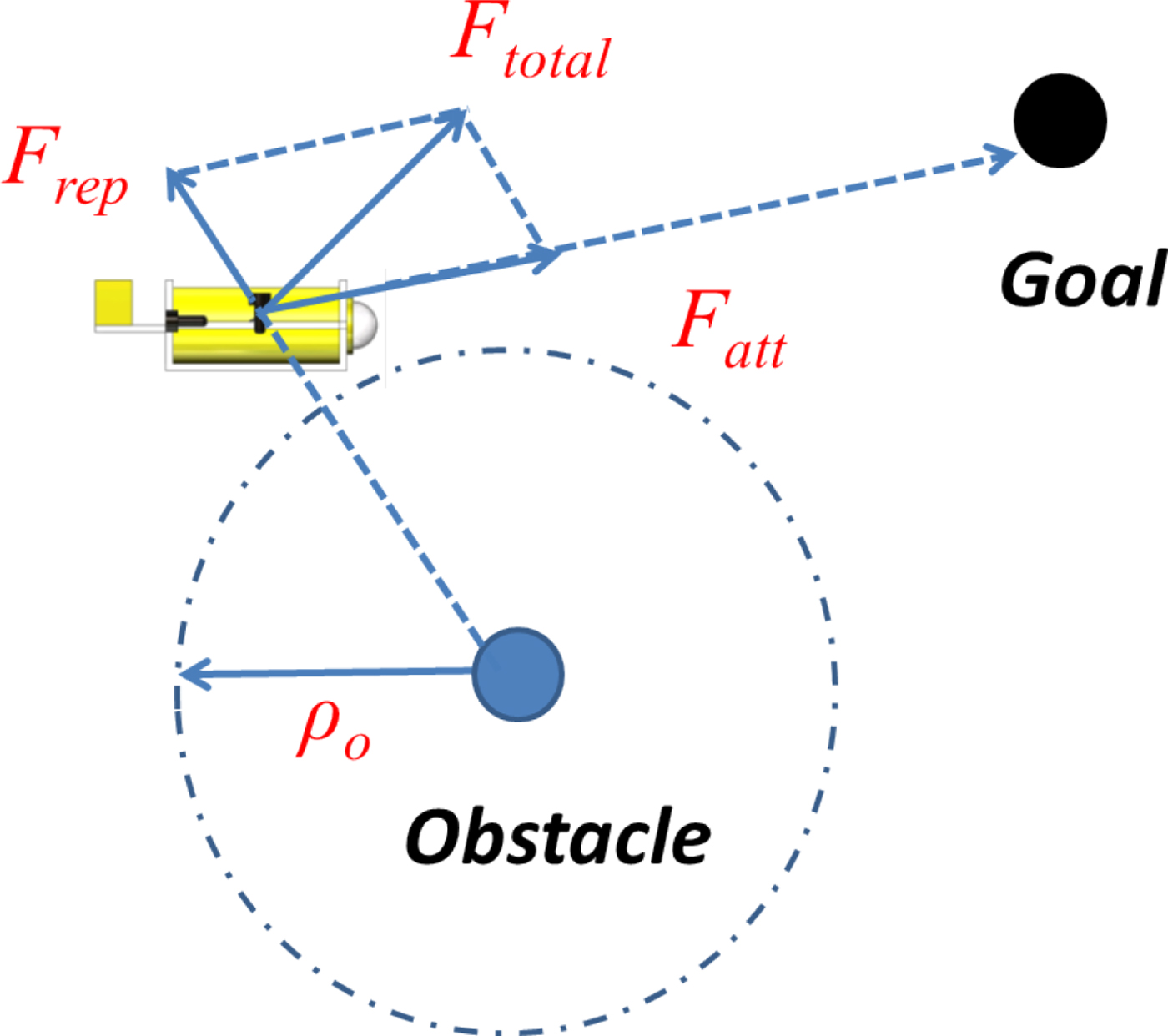
The APFM is a path planning algorithm introduced by Khatib (Reference Khatib1986). With a simple numerical model suitable for real-time obstacle avoidance and navigation, the APFM has seen widespread use in unmanned ground vehicles. For AUV applications, a virtual potential field must be defined, in which the AUV, Goal, and Obstacle are treated as different points. The Goal has an attractive field, and the Obstacle has a repulsive field. As shown in Figure 1, the AUV moves towards the Goal under its attractive force, and away from the Obstacle under its repulsive force; thus, the AUV moves in the direction of the resultant (of the attractive and repulsive vectors).

Figure 1. Artificial potential field.
Assuming the position of the AUV is X i = (x, y), the function for the Goal's attractive field can be defined as follows:
 $$U_{att} \lpar X_{i}\rpar =\displaystyle{{1}\over{2}}\alpha \rho^{2}\lpar X_{i} \comma \; X_{g}\rpar$$
The function for the Obstacle's repulsive field is as follows:
 $$U_{rep} \lpar X_{i}\rpar =\left\{\matrix{\displaystyle{{1}\over{2}}\beta \left(\displaystyle{{1}\over{\rho \lpar X_{i}\comma \; X_{o}\rpar }}-\displaystyle{{1}\over{\rho_{o}}}\right)^{2} \hfill &\rho \lpar X_{i}\comma \; X_{o}\rpar \le \rho_{0} \hfill \cr 0 \hfill &\rho \lpar X_{i}\comma \; X_{o}\rpar \gt \rho_{0}\hfill}\right.$$
where: α and β are the gain factors for the attractive force and repulsive force, respectively; X i, X g, and X o are the spatial positions of the AUV, Goal and Obstacle, respectively;  $\rho \lpar X_{i}\comma \; X_{g}\rpar $ and
  $\rho \lpar X_{i}\comma \; X_{o}\rpar $ are the spatial distances from the AUV to the Goal and Obstacle, respectively and ρo is the Obstacle's radius of influence on the AUV, which is not effective when the AUV is not within the repulsive field.
By calculating the negative gradient of the attractive and repulsive fields, the corresponding attractive function and repulsive function can be obtained as follows:
Attractive function:
 $$F_{att} \lpar X_{i}\rpar =-\nabla U_{att} \lpar X_{i}\rpar =\alpha \rho \lpar X_{i}\comma \; X_{g}\rpar$$
Repulsive function:
 $$\eqalign{F_{rep} \lpar X_{i}\rpar &=-\nabla U_{rep} \lpar X_{i}\rpar \cr &= \left\{\matrix{\beta \left(\displaystyle{{1}\over{\rho \lpar X_{i}\comma \; X_{o}\rpar }}-\displaystyle{{1}\over{\rho_{o}}}\right)\displaystyle{{1}\over{\rho^{2}\lpar X_{i}\comma \; X_{o}\rpar }}\comma \;\hfill &\rho \lpar X_{i}\comma \; X_{o}\rpar \le \rho_{0} \hfill \cr 0\comma \; \hfill &\rho \lpar X_{i}\comma \; X_{o}\rpar \gt \rho_{0} \hfill}\right.}$$
Hence, the resultant force on the AUV is as follows:
 $$F_{total} \lpar X_{i}\rpar =F_{att} \lpar X_{i}\rpar +F_{rep} \lpar X_{i}\rpar$$
The depth-control algorithm and altitude control algorithm for the AUV's obstacle avoidance and bottom-following operations are derived from these basic principles.
2.2. Depth-control algorithm
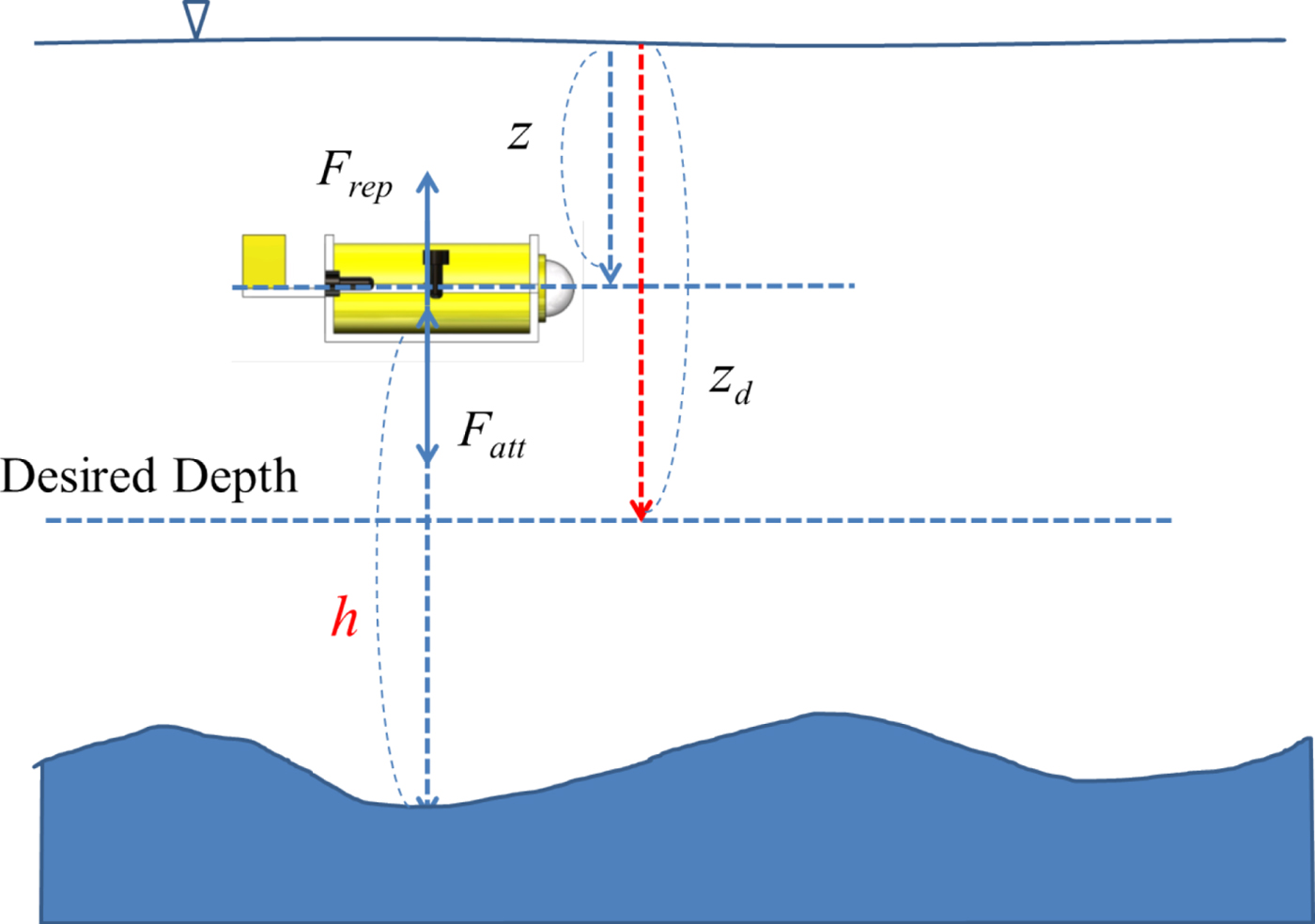
As per the APFM, the depth-control algorithm defines the attractive field as a depth function and the repulsive field as an altitude function, with a predetermined minimal safe altitude for obstacle avoidance. The AUV approximates a desired depth according to the resultant force of the attractive and repulsive forces, so as to prevent collisions with the seabed and obstacles. As shown in Figure 2, the virtual force only works along the z-axis. The desired depth defines an attractive field; the AUV is attracted to the desired depth; conversely, an obstacle has a repulsive field, whose repulsive force only works on the AUV when it comes into range; otherwise, the AUV will only be subjected to the attractive force. The depth-control function for the attractive potential field can be defined as (Gao et al., Reference Gao, Xu, Zhao and Yan2008):

Figure 2. Depth control.
 $$U_{att} \lpar z\rpar = \left\{\matrix{k_{az} \vert z-z_{d} \vert \comma \; \hfill &\vert z-z_{d}\vert \gt l_{z} \hfill \cr \displaystyle{{k_{az}}\over{2l_{z}}}\lpar z-z_{d}\rpar^{2}\comma \; \hfill &\vert z-z_{d} \vert \le l_{z} \hfill}\right.$$
where: z is the depth of the AUV; z d is the desired depth; k az is the gain value of the attractive force and l z is the attraction switching condition such that, when the difference between z and z d is larger than l z, a linear function holds; otherwise, the standard quadratic function for the artificial potential field is used.
The attractive force is the negative gradient of the attractive potential field, and it can be defined as follows:
 $$\eqalign{F_{att} \lpar z\rpar &= -\nabla U_{att} \lpar z\rpar \cr &= \left\{\matrix{-k_{az} \hbox{sgn}\lpar z-z_{d}\rpar \comma \; \hfill &\vert z-z_{d}\vert \gt l_{z} \hfill \cr - \displaystyle{{k_{az}}\over{l_{z}}}\lpar z-z_{d}\rpar \comma \; \hfill &\vert z-z_{d} \vert \le l_{z} \hfill}\right.}$$
When the AUV is close to the seabed, it is repelled by the repulsive field, defined as:
 $$U_{rep} \lpar h\rpar = \left\{\matrix{\displaystyle{{1}\over{2}}k_{rh}\left(\displaystyle{{1}\over{h}}-\displaystyle{{1}\over{h_{0}}}\right)^{2}\comma \; \hfill &0 \lt h\le h_{0} \hfill \cr 0\comma \; \hfill &h \gt h_{0} \hfill}\right.$$
where: h is the altitude from the seabed to the AUV; k rh is the gain value of the repulsive force and h 0 is the range of the repulsive field. When h > h 0, the AUV is out of range of the repulsive force.
The repulsive force is the negative gradient of the repulsive potential field; it can be defined as follows:
 $$\eqalign{F_{rep} \lpar h\rpar &=-\nabla U_{rep} \lpar h\rpar \cr &=\left\{\matrix{k_{rh} \left(\displaystyle{{1}\over{h}}-\displaystyle{{1}\over{h_{o}}}\right)\displaystyle{{1}\over{h^{2}}}\comma \; \hfill &0 \lt h\le h_{0} \hfill \cr 0\comma \; \hfill &h \gt h_{0} \hfill} \right.}$$
Combining the attractive and repulsive forces yields the resultant force:
 $$F_{total} =F_{att} \lpar z\rpar +F_{rep} \lpar h\rpar$$
The AUV controls its depth according to the resultant force, which can be defined as the following function:
 $$z_{com} =k_{z} F_{total}$$
where z com is the depth-control command for the AUV, and k z is the scale factor for the depth-control command.
2.3. Altitude-control algorithm
The altitude-control algorithm defines the attractive field as an altitude function, and the repulsive field a depth function, with a predetermined maximum operating depth for the AUV. The AUV maintains its altitude according to the resultant force it is subjected to, so that when the AUV conducts bottom following at a fixed altitude, it will not descend lower than a structurally safe depth.
As shown in Figure 3, h d represents the desired altitude for the AUV bottom following. The AUV moves to h d because h d attracts the AUV. The maximum operating depth is defined as a repulsive field, which prevents the AUV from descending below its depth limit.
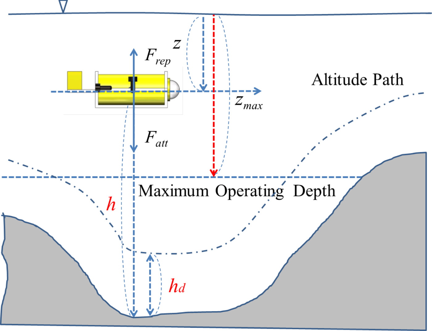
Figure 3. Altitude control.
The altitude-control attractive function can be defined as (Gao et al., Reference Gao, Xu, Zhao and Yan2008):
 $$U_{att} \lpar h\rpar =\left\{\matrix{k_{ah} \vert h-h_{d} \vert \comma \; \hfill &\vert h-h_{d} \vert \gt l_{h} \hfill \cr \displaystyle{{k_{ah}}\over{2l_{h}}}\lpar h-h_{d}\rpar^{2}\comma \; \hfill &\vert h-h_{d} \vert \le l_{h} \hfill}\right.$$
where: h d is the desired altitude; k ah is the gain value of the attractive force, and l h is the condition for the switching of the attractive function. When the difference between h and h d is larger than l h, the attractive function is linear; otherwise, it is a standard quadratic function for the artificial potential field.
The attractive force is the negative gradient of the attractive field, and it can be defined as follows:
 $$\eqalign{F_{att} \lpar h\rpar &=-\nabla U_{att} \lpar h\rpar \cr &= \left\{\matrix{-k_{ah} \hbox{sgn}\lpar h-h_{d}\rpar \comma \; \hfill &\vert h-h_{d}\vert \gt l_{h} \hfill \cr -\displaystyle{{k_{ah}}\over{l_{h}}}\lpar h-h_{d}\rpar \comma \; \hfill &\vert h-h_{d}\vert \le l_{h} \hfill}\right.}$$
In light of the structural strength of the AUV, its maximum operating depth must be adopted as the repulsive field, to prevent the AUV from diving below its depth limit. The repulsive function can be defined as (Gao et al., Reference Gao, Xu, Zhao and Yan2008):
 $$U_{rep} \lpar z\rpar =\left\{\matrix{\displaystyle{{k_{rz}}\over{2}}\left(\displaystyle{{1}\over{z_{\max} -z}}-\displaystyle{{1}\over{r_{0}}}\right)^{2}\comma \; \hfill &0 \lt z_{\max} -z\le r_{o} \hfill \cr 0\comma \; \hfill &z_{\max} -z \lt r_{0} \hfill}\right.$$
where: z max is the maximum operating depth; k rz is the gain value of the repulsive force and r 0 is the radius of the repulsive field.
The repulsive force is defined as:
 $$\eqalign{F_{rep} \lpar z\rpar &=-\nabla U_{rep} \lpar z\rpar \cr &= \left\{\matrix{-k_{rz} \left(\displaystyle{{1}\over{\lpar z_{\max} -z\rpar }}-\displaystyle{{1}\over{r_{0}}}\right)\displaystyle{{1}\over{\lpar z_{\max} -z \rpar^{2}}}\comma \; \hfill &0 \lt z_{\max} -z\le r_{0} \hfill \cr 0\comma \; \hfill &z_{\max} -z \gt r_{0} \hfill}\right.}$$
The resultant force on the AUV is shown as follows:
 $$F_{total} =F_{att} \lpar h\rpar +F_{rep} \lpar z\rpar$$
As the AUV maintains its altitude according to the resultant force, the operation can be represented by a simple linear function as follows:
 $$h_{com} =k_{h} F_{total}$$
where h com is the altitude-control command for the AUV and k h is the scale factor for the altitude-control command.
2.4. H∞ control theory
Obstacle avoidance and seabed following must be planned with the APFM and conducted with the H∞ controller, because the H∞ controller's robustness allows it to suppress external interference, maintain system stability and sustain precise control. The H∞ controller allows the minimal ∞ norm for the transfer function from the exogenous inputs and the controlled outputs and stabilises the entire closed-loop system. The ∞ norm can be defined as follows (Doyle et al., Reference Doyle, Glover, Khargonekar and Francis1989):
 $$\Vert G \Vert _{\infty } \equiv \sup\limits_{\omega}\ \bar{\sigma} [G (j \omega)]$$
where: G(s) is the transfer function of the system; sup is the least upper bound; and  $\bar{\sigma}$ is the maximum singular value of G(s), which is the least upper bound of the transfer function's maximum singular values for all frequencies.
The equations of state for this linear time-invariant system G(s) are as follows:
 $$\eqalign{\dot{X}\lpar t\rpar &= AX\lpar t\rpar +Bu\lpar t\rpar \cr y_{S} \lpar t\rpar &=CX\lpar t\rpar +Du\lpar t\rpar }$$
where: X is the system's state variables; u is the control input; y s is the plant output; and A, B, C and D are constant matrices. Three weight functions are added to the system to form an augmented system P(s) as shown in Figure 4, in which the three weight functions are defined as follows:

Figure 4. Augmented system.
 $$W_{1} = \left[\matrix{A_{W1} &B_{W1} \cr C_{W1} &D_{W1}}\right]\comma \; \quad W_{2} =\left[\matrix{A_{W2} &B_{W2} \cr C_{W2} &D_{W2}}\right]\comma \; \quad W_{3} =\left[\matrix{A_{W3} &B_{W3} \cr C_{W3} &D_{W3}}\right]$$
This augmented system can be expressed in a standard control framework, as shown in Figure 5, where the controlled output Z(t) includes the tracking error e(t), control input u(t), and plant output y s(t); and the exogenous input R(t) includes the reference signal r(t), external interference d(t) and sensor noise n(t). The controlled output and exogenous input can be expressed as follows:
Figure 5. Standard control framework.
 $$R\lpar t\rpar \equiv \left[\matrix{r\lpar t\rpar \cr d\lpar t\rpar \cr n\lpar t\rpar }\right]\comma \; \quad z\lpar t\rpar \equiv \left[\matrix{z_{1} \lpar t\rpar \cr z_{2} \lpar t\rpar \cr z_{3} \lpar t\rpar }\right]=\left[\matrix{W_{1} e\lpar t\rpar \cr W_{2} u\lpar t\rpar \cr W_{3} y_{S} \lpar t\rpar }\right]$$
The augmented system can be expressed as a state matrix:
 $$\left[\matrix{\dot{X} \cr \dot{X}_{W_{1}} \cr \dot{X}_{W_{2}} \cr \dot{X}_{W_{3}} \cr z_{1} \cr z_{2} \cr z_{3} \cr e}\right]=\left[\matrix{A &0 &0 &0 &0 &B \cr -B_{W_{1}} &A_{W_{1}} &0 &0 &B_{W_{1}} &-B_{W_{1}} D \cr 0 &0 &A_{W_{2}} &0 &0 &B_{W_{2}} \cr B_{W_{3}} C &0 &0 &A_{W_{3}} &0 &B_{W_{3}} D \cr -D_{W_{1}} C &C_{W_{1}} &0 &0 &D_{W_{1}} &-D_{W_{1}} D \cr 0 &0 &C_{W_{2}} &0 &0 &D_{W_{2}} \cr D_{W_{3}} C &0 &C_{W_{3}} &0 &0 &D_{W_{3}} D \cr -C &0 &0 &0 &I &-D}\right]\left[\matrix{X \cr X_{W_{1}} \cr X_{W_{2}} \cr X_{W_{3}} \cr R \cr u}\right]$$
which can be simplified into the following:
 $$\left[\matrix{\dot{X}\lpar t\rpar \cr Z\lpar t\rpar \cr e\lpar t\rpar }\right]=\left[\matrix{A &B_{1} &B_{2} \cr C_{1} &D_{11} &D_{12} \cr C_{2} &D_{21} &D_{22}}\right]\left[\matrix{X\lpar t\rpar \cr R\lpar t\rpar \cr u\lpar t\rpar }\right]$$
where A, B 1, B 2, C 1, C 2, D 11, D 12, D 21 and D 22 are all constant matrices.
It can then be reformed as follows:
 $$\left[\matrix{z_{1} \cr z_{2} \cr z_{3} \cr \ldots \cr e}\right]=\left[\matrix{W_{1} &-W_{1} G &-W_{1}&\vdots &-W_{1} G \cr 0 &0 &0 &\vdots &W_{2} \cr 0 &W_{3} G &0 &\vdots &W_{3} G \cr \ldots &\ldots &\ldots &\ldots &\ldots \cr I &-G &-I &\vdots &-G}\right]\left[\matrix{r \cr d \cr n \cr \ldots \cr u}\right]$$
or simplified to:
 $$\left[\matrix{Z\lpar s\rpar \cr \ldots \ldots \cr e\lpar s\rpar }\right]=\left[\matrix{P_{11} \lpar s\rpar &\vert &P_{12} \lpar s\rpar \cr ---- &- &---- \cr P_{21} \lpar s\rpar &\vert &P_{22} \lpar s\rpar }\right]\left[\matrix{R\lpar s\rpar \cr \ldots\ldots \cr u\lpar s\rpar }\right]$$
 As the transfer function  $u\lpar s\rpar =K\lpar s\rpar \cdot e\lpar s\rpar $, this gives the following relations:
 $$Z\lpar s\rpar =P_{11} \lpar s\rpar \cdot R\lpar s\rpar +P_{12} \lpar s\rpar \cdot K\lpar s\rpar \cdot e\lpar s\rpar$$
 $$e\lpar s\rpar =P_{21} \lpar s\rpar \cdot R\lpar s\rpar +P_{22} \lpar s\rpar \cdot K\lpar s\rpar \cdot e\lpar s\rpar$$
 $$\Rightarrow e\lpar s\rpar =\lpar I-P_{22} \lpar s\rpar \cdot K\lpar s\rpar \rpar ^{-1}P_{21} \lpar s\rpar \cdot R\lpar s\rpar$$
Substituting Equation (28) into Equation (26) yields:
 $$Z= [P_{11} +P_{12} \cdot K\lpar I-P_{22} \cdot K\rpar ^{-1}P_{21}] \cdot R$$
The linear fraction transformation F 1(P, K) of the transfer function from R(s) to Z(s) can be expressed as follows:
 $$F_{l} \lpar P\comma \; K\rpar =P_{11} +P_{12} K [I-P_{22} K]^{-1}P_{21}$$
The H∞ controller allows the minimal H∞ norm for the transfer function F l(P, K) from the exogenous inputs and the controlled outputs; it stabilises the entire closed-loop system. Therefore, for the H∞ norm for the transfer function F l(P, K), a value smaller than γ should be defined as follows:
 $$\Vert F_{l} \lpar P\comma \; K\rpar \Vert _{\infty} =\sup\limits_{\omega \lpar t\rpar } \displaystyle{{\Vert Z \Vert _{2}}\over{\Vert R \Vert _{2}}} \lt \gamma$$
 Usually γ is a value smaller than one and bears the physical meaning that the energy  $\lpar \Vert R \Vert _{2}\rpar $ of the exogenous input is transformed by the controller, and the energy
  $\lpar \Vert Z \Vert _{2}\rpar $ of the system output is γ times lower than the input energy
  $\Vert R \Vert _{2}$.
Hwang (Reference Hwang1993; Reference Hwang2002) proposed a polynomial approach to the H∞ control problem. It is relatively simple and convenient in calculation, because it only requires the positive definite solutions of two Riccati equations. The system's equations of state are as follows:
 $$\eqalign{\dot{X}\lpar t\rpar &=AX\lpar t\rpar +B_{1} w\lpar t\rpar +B_{2} u\lpar t\rpar \cr Z\lpar t\rpar &=C_{1} X\lpar t\rpar +D_{12} u\lpar t\rpar \cr e\lpar t\rpar &=C_{2} X\lpar t\rpar +D_{21} w\lpar t\rpar }$$
Polynomial approaches must meet the following conditions:
(i) (A, B1) must be stabilisable, and (C1, A) must be detectable;
(ii) (A, B2) must be stabilisable, and (C2, A) must be detectable;
(iii)
 $D_{12}^{T} D_{12} =I$, and $D_{21} D_{21}^{T} =I$.


To obtain the solution for the H∞ controller, the gain for state feedback control K c and the observer gain K f must be acquired first (Doyle et al., Reference Doyle, Glover, Khargonekar and Francis1989; Hwang, Reference Hwang1993):
 $$K_{c} =-\lpar B_{2}^{T} k_{\infty} X+D_{12}^{T} C_{1}\rpar$$
 $$K_{f} =-\lpar I-h_{\infty } k_{\infty}\rpar ^{-1}\lpar h_{\infty} C_{2}^{T} +B_{1} D_{21}^{T} \rpar$$
where k ∞ and h ∞ are the positive definite solutions for the following Riccati equations, respectively:
 $$\eqalign{&\lpar A-B_{2} D_{12}^{T} C_{1}\rpar ^{T}k_{\infty } +k_{\infty } \lpar A-B_{2} D_{12}^{T} C_{1} \rpar +k_{\infty } \lpar B_{1} B_{1}^{T} -B_{2} B_{2}^{T}\rpar k_{\infty} \cr &\quad +C_{1}^{T} \lpar I-D_{12} D_{12}^{T}\rpar \lpar I-D_{12} D_{12}^{T}\rpar C_{1} =0}$$
 $$A_{t} h_{\infty } +h_{\infty } A_{t}^{T} +h_{\infty} \lpar C_{1}^{T} C_{1} -C_{2}^{T} C_{2} \rpar h_{\infty } +B_{1t} B_{1t}^{T} =0$$
and:
 $$A_{t} =A-B_{1} D_{21}^{T} C_{2}\comma \; \quad B_{1t} =B_{1} \lpar I-D_{21}^{T} D_{21}\rpar$$
Then, the optimal H∞ control is as follows:
 $$K\lpar s \rpar =\left[{A+B_{1} B_{1}^{T} k_{\infty} +B_{2} K_{c} +K_{f} C_{2} \over K_{c}}\!\!{\vert \over \vert}\!\!{-K_{f} \over 0}\right]$$
For a standard feedback control system whose plant is G(s) and whose controller is K(s), the sufficient condition for its stability is as follows:
 $$\Vert KG\Vert _{\infty} \lt 1$$
 The stability and performance of the closed-loop system can be defined by the sensitivity function  $S =1/\lpar I+GK\rpar $, power transfer function
  $P = K/\lpar I+GK\rpar $, and complementary sensitivity function
  $T =GK/\lpar I+GK\rpar $. Therefore, suitably designed weight functions that allow favourable singular values for sensitivity, complementary sensitivity and power transfer must be introduced to attain the required system performance, favourable robustness, tracking ability and noise elimination capacity. To this end, the following conditions must be satisfied:
 $$\eqalign{&\Vert SW_{1} \Vert _{\infty} \le 1 \cr &\Vert PW_{2} \Vert _{\infty} \le 1 \cr &\Vert TW_{3} \Vert _{\infty} \le 1}$$
3. SIMULATION ANALYSIS
3.1. AUV Motion in the vertical plane
This study of AUV motion concentrates on the control for vertical movements and only the equations of the heave must be addressed (Fang et al., Reference Fang, Chang and Luo2006; Reference Fang, Hou and Luo2007).
 $$\eqalign{&\lpar m-Z_{\dot{w}}\rpar \dot{w}+my_{G} \dot{p}-mx_{G} \dot{q} \cr &\quad = mz_{G} \lpar p^{2}+q^{2}\rpar -mr\lpar x_{G} p+y_{G} q\rpar +q\lpar m-X_{\dot{u}}\rpar u-p\lpar m-Y_{\dot{v}}\rpar v \cr &\qquad +\lpar Z_{w} +Z_{w\vert w \vert } \vert w \vert \rpar w+\lpar W-B\rpar \cos \theta \cos \phi +F_{z}}$$
where: the inertia and added mass term is  $\lpar m-Z_{\dot{w}}\rpar \dot{w}+my_{G} \dot{p}-mx_{G} \dot{q}$; the centripetal force term is
  $mz_{G} \lpar p^{2}+q^{2}\rpar -mr\lpar x_{G} p+y_{G}q\rpar $; the Coriolis force term is
  $q\lpar m-X_{\dot{u}}\rpar u-p\lpar m-Y_{\dot{v}}\rpar v$; the damping force term is
  $\lpar Z_{w} +Z_{w\vert w \vert } \vert w \vert \rpar w$; the restoring force term is
  $\lpar W-B\rpar \cos \theta \cos \phi $ and the external force term is F z.
A self-developed AUV has been designed and built at the Cheng Kung University, which is  $1{\cdot}1 \times 0{\cdot}385 \times 0{\cdot}35$ m in size. The specifications of the AUV are listed in Table 1, and the hydrodynamic coefficients for added mass and damping measured through the Planar Motion Mechanism (PMM) are as listed in Table 2 (Fang et al., Reference Fang, Wang, Wu and Lin2015).
Table 1. Specifications of the AUV.
Table 2. Added Mass and Fluid Damping Coefficients.
In Tables 1 and 2, m is the mass; W is the weight; B is the buoyancy; I x, I y, I z, I xy and I yz are the inertia moments;  $\dot{u}\comma \; \enspace \dot{v}\comma \; \enspace \dot{w}\comma \; \enspace \dot{p}\comma \; \enspace \dot{q}$ and
  $\dot{r}$ are the linear accelerations and angular accelerations along the three axes of the body coordinate system;
  $X_{\dot{u}}$,
  $Y_{\dot{v}}$,
  $Z_{\dot{w}}$,
  $K_{\dot{p}}$,
  $M_{\dot{q}}$ and
  $N_{\dot{r}}$ are the hydrodynamic coefficients of added mass; X u, Y v, Z w, K p, M q and N r are the linear damping coefficients;
  $X_{u\vert u \vert }$,
  $Y_{v\vert v \vert }$,
  $Z_{w\vert w \vert }$,
  $K_{p\vert p \vert }$,
  $M_{q\vert q \vert } $ and
  $N_{r\vert r \vert } $ are the quadratic damping coefficients and F x, F z and M z are the horizontal axial thrust, vertical axial thrust, and horizontal turning moment, respectively. The centre of gravity is
  $\lpar x_{G}\comma \; y_{G}\comma \; z_{G}\rpar $ and the centre of buoyancy is
  $\lpar x_{B}\comma \; y_{B}\comma \; z_{B}\rpar $.
3.2. Design of the H∞ controller
By substituting the specifications and coefficients of the AUV in Tables 1 and 2 into the aforementioned dynamic equation, it can be simplified into the following matrices:
 $$\eqalign{\left[\matrix{\dot{w} \cr \dot{z}}\right]&=\left[\matrix{-0.96-1.47\vert w \vert &0 \cr 1 &0}\right]\left[\matrix{w \cr z}\right]+\left[\matrix{0.0095 \cr 0}\right]F_{z} \cr y_{d} &=\left[\matrix{0 &1}\right]\left[\matrix{w \cr z}\right]}$$
where the state variables are w and z, which are the rate of diving and depth of the AUV, respectively; F z is the control input and y d is the measurement output.
We set the weight functions W 1, W 2 and W 3 as:
 $$W_{1} =\displaystyle{{10}\over{100s+1}}\comma \; \quad W_{2} =\displaystyle{{1}\over{1000}}\comma \; \quad W_{3} =\displaystyle{{s+550}\over{300s+800}}$$
The original system is augmented with those weight functions; the gain for state feedback control K cl and the observer gain K fl can be obtained from the MATLAB simulation as follows:
When  $\gamma = 0.9758$,
 $$\eqalign{K_{c1} &=\left[\matrix{2233 &-981 &-2652 &-476}\right]\cr K_{f1} &=\left[\matrix{-0.4384 &0 &0.0351 &0.0132}\right]^{T}}$$
the robust controller is:
 $$K\lpar S\rpar =\left[\matrix{ak &bk \cr ck &dk}\right]$$
where:
 $$\eqalign{ak &= \left[\matrix{-0.01 &0 &0 &0 \cr 9.298 &-5.045 &-11.043 &-1.983 \cr 0 &1 &-0.08 &0.211 \cr 0 &0 &0.97 &-2.587}\right]\comma \; \quad bk=\left[\matrix{0.4384 \cr 0 \cr -0.0351 \cr -0.0132}\right]\cr ck &= \left[\matrix{2233 &-981 &-2652 &-476}\right]\comma \; \quad dk= [0]}$$
Then, the transfer function for the robust controller K(s) can be expressed as:
 $$\eqalign{K\lpar s\rpar &=\displaystyle{{1078\, s^{3}+3912\, s^{2} + 2766\, s + 4.031} \over {s^{4}+7.722\, s^{3} + 24.58\, s^{2} + 30.75\, s + 0.3051}} \cr &= \displaystyle{{1078.16 \lpar s+2.667\rpar \lpar s+0.96\rpar \lpar s+0.00146\rpar }\over{\lpar s+2.885\rpar \lpar s+0.01\rpar \lpar s^{2} +4.827s + 10.58\rpar }}}$$
3.3. Frequency-domain response simulation
The depth-control frequency-domain response simulation of the H∞ controller yielded the relationship between weight and singular values of system sensitivity shown in Figure 6. The open-loop system KG satisfies the restrictions of W 1 at low frequencies and the restrictions of W 3 at high frequencies. After W 1 had been determined, the singular values of its sensitivity function were under the reciprocal of W 1 (i.e.  $W_{1}^{-1}\rpar $, satisfying the requirements for bottom following. When W 2 was set to be constant and the capacity of the thrusters was restricted, the curve of the singular values showed that the singular values of power transfer function R were under the reciprocal of W 2 (i.e.
  $W_{2}^{-1}\rpar $, satisfying the requirements. The power function R was able to prevent system saturation. After W 3 had been determined, the singular values of the complementary sensitivity function were all under the reciprocal of W 3 (i.e.
  $W_{3}^{-1} \rpar $, meaning the system resisted noise. Because the noise received by the sensor mostly originated from high-frequency signals, such as electromagnetic interference phenomena and the AUV's vibrations, the complementary sensitivity function T must generate low values at high frequencies to counteract noise.
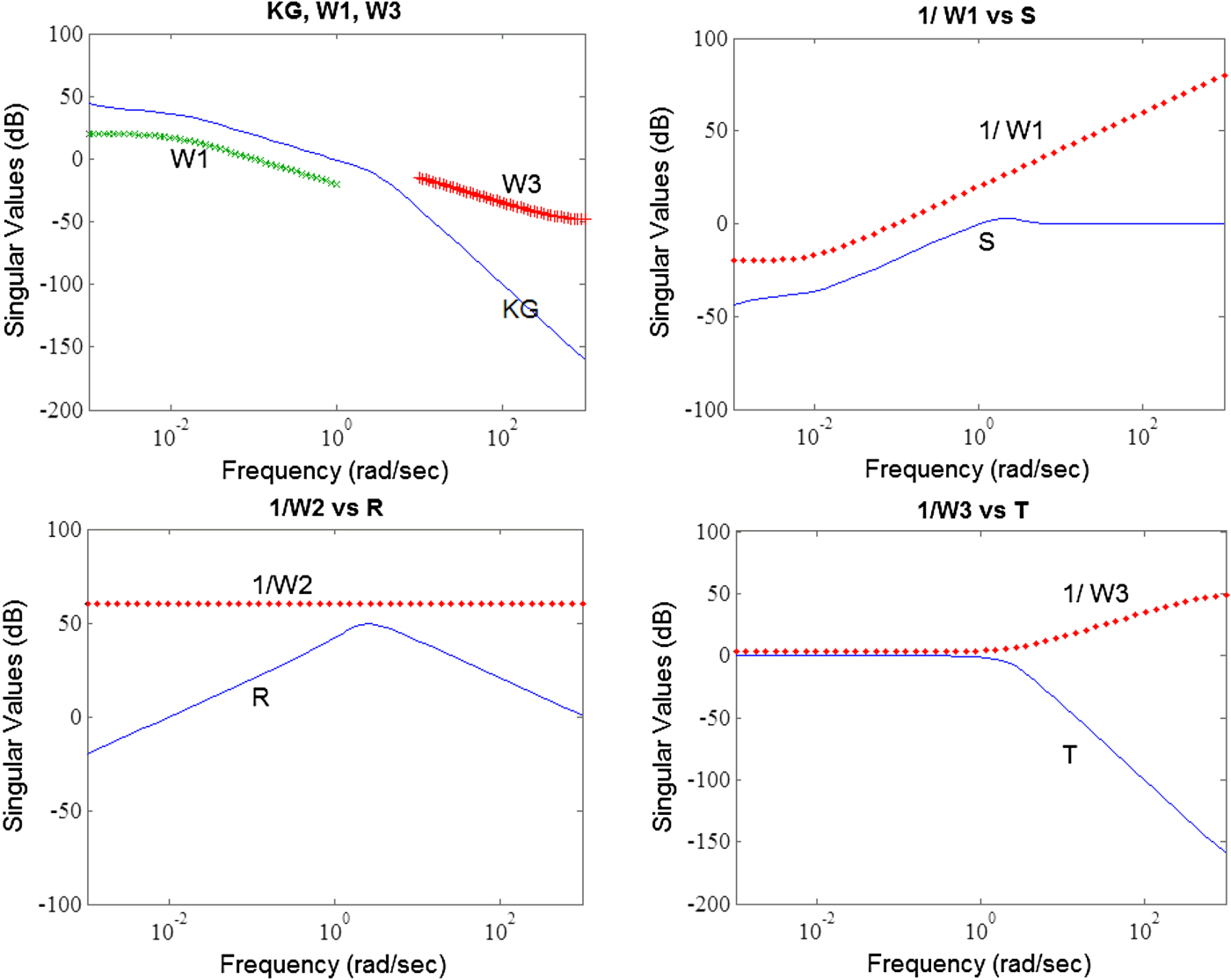
Figure 6. Results of frequency-domain response simulations for the H∞ controller.
3.4. Noise interference simulation
In a noise interference simulation, the performance of an H∞ controller and a Proportional Integral Derivative (PID) controller were compared; both were based on the system dynamics of the AUV and underwent adequate parameter adjustments. Figures7(a), 7(c) and 7(e) show the contrast after adding an external interference signal 2sin(t); the H∞ controller was robust and was only slightly influenced by the interference, unlike the PID controller, which jittered noticeably. Figures7(b), 7(d) and 7(f) show the addition of random interference, which also corroborated the robustness of the H∞ controller.
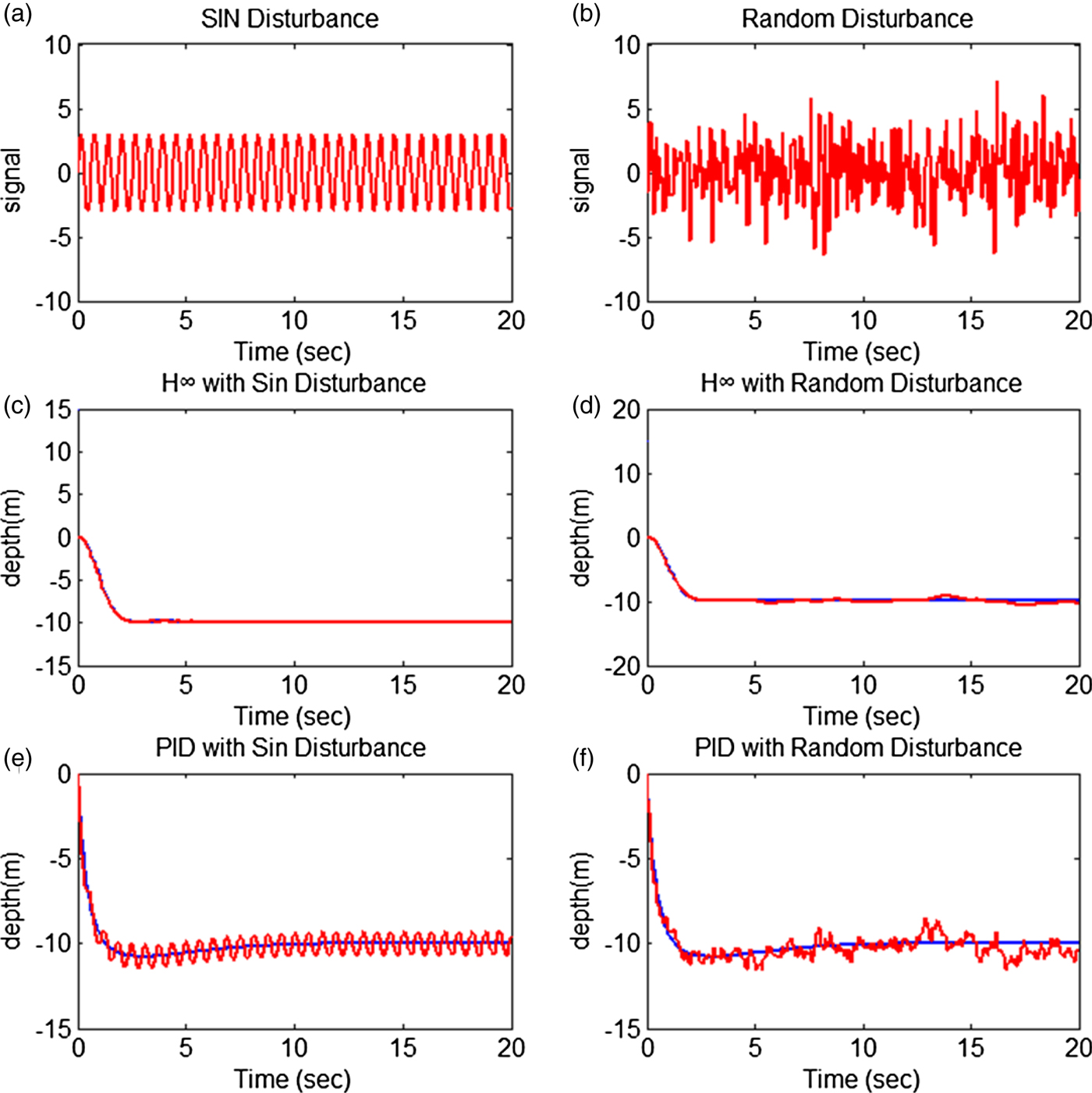
Figure 7. Comparison of the H∞ controller and PID controller under external interference.
3.5. Control simulation
Owing to the varying contours of the seabed, the H∞ controller must issue different depth or altitude control commands for the AUV to conduct precision tracking. Simulations tested the depth control and altitude control algorithms:
3.5.1. Depth control simulations
3.5.1.1. Case 1: Obstacle avoidance at − 5 m depth
In this simulation, the AUV negotiated the varying contours of a seabed; conditions were as follows: AUV speed = 0·5 m/sec; k az (gain value of the attractive force) = 0·5; l z (condition for the switching of attractive function) = 2 m; k rh (gain value of the repulsive force) = 0·8; h 0 (range of the repulsive field) = 5 m; and z d (desired depth) =− 5 m. In Figure 8, the black dashed line represents the seabed profile, the red solid line the AUV depth trajectory, and the blue dotted line the AUV altitude. Judging from the AUV depth trajectory (red line), initially, the AUV was subjected to a constant attractive force and dived at a steady speed, until the difference between the AUV depth and the decided depth is not larger than 2 m, the attractive force acted by the standard quadratic function of the artificial potential field. At that moment, because the sea bottom was some distance away, the influence of the repulsive force was negligible and the AUV cruised at a fixed depth, until the rise of the seabed (x = 20~30) caused an escalation in repulsive force, which in turn compelled the AUV to change its course and ascend, until it passed the obstacle and returned to the original desired depth.

Figure 8. Obstacle avoidance simulation at − 5 m depth.
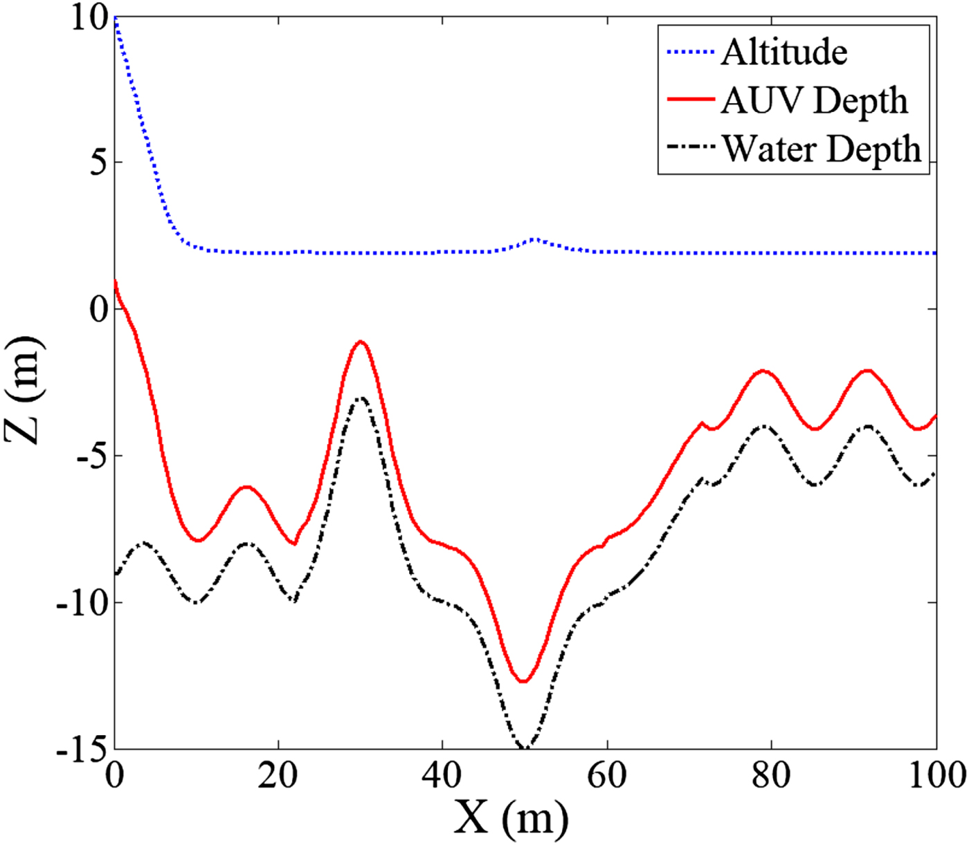
3.5.1.2. Case 2: Obstacle avoidance at − 7 m depth
In this simulation, the conditions were the same as those of Case 1, except that the desired depth was −7 m. Figure 9 presents the results. The AUV depth trajectory (red line) initially dived but reached the repulsive field before reaching the desired depth; as the AUV approached the bottom, the repulsive force surpassed the attractive force, and the resultant force compelled the AUV to adjust its depth; thus, it cruised above the seabed instead of crashing into it. Later, midway through the operation, the terrain became a downward slope, which increased the depth of the sea bottom and decreased the repulsive force; the attractive force again brought the AUV downward to the desired depth. When the terrain rose again, the escalating repulsive force compelled the AUV to climb up quickly to prevent collision, until it reached a shallow shelf, where it cruised at a fixed depth and accomplished the obstacle avoidance mission. The simulation results clearly indicate that the proposed APFM was able to maintain effective depth control and was able to keep the AUV above the bottom in shallow water, so as to prevent collision with the seabed. Additionally, it was able to quickly bring the AUV over a suddenly rising precipice. As for the problem of local minima, although the AUV was not able to reach any specified depth that was too close to the bottom, this apparent drawback is actually a feature because it serves as a safety measure that prevents the AUV from hitting the seabed.
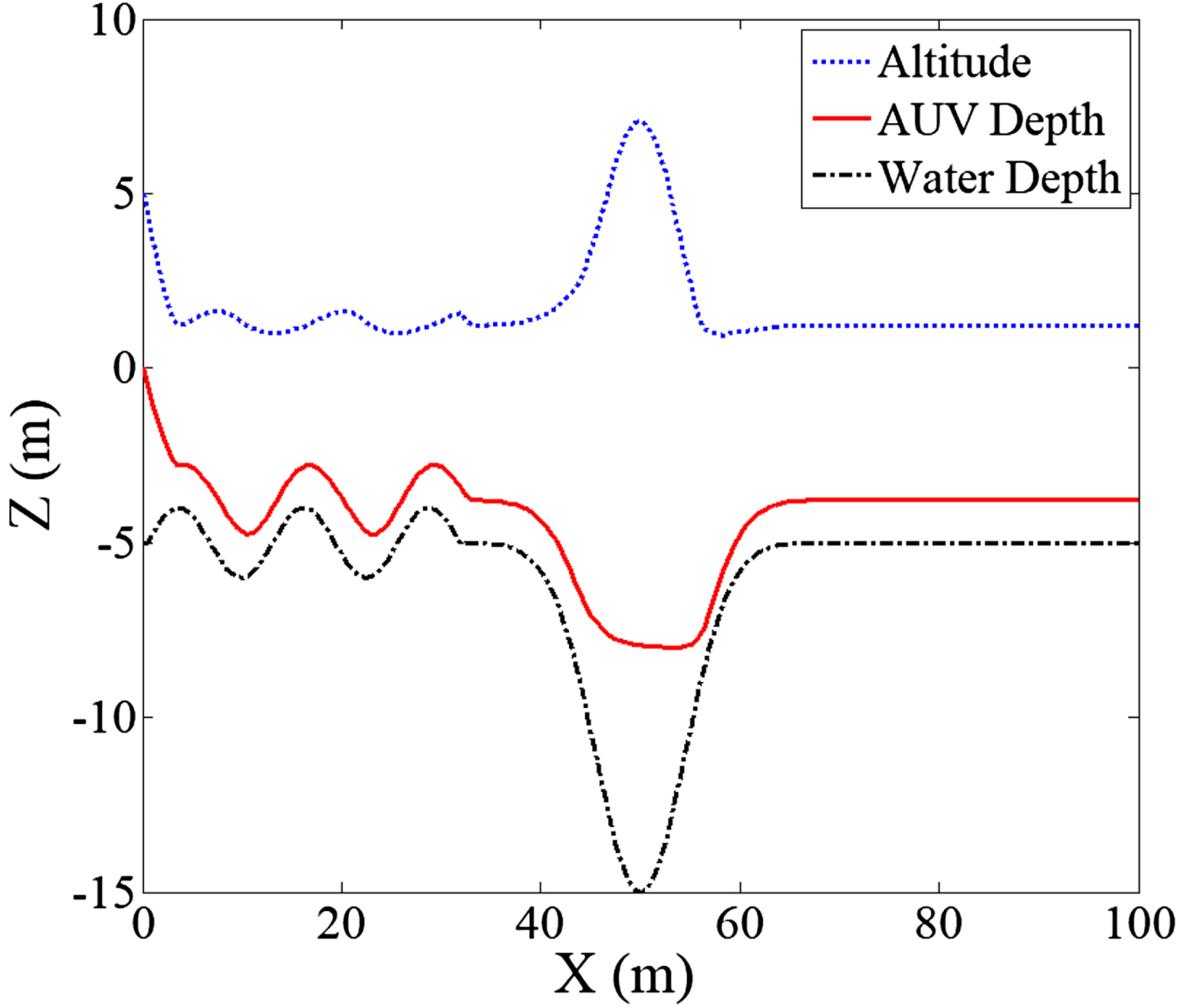
Figure 9. Obstacle avoidance simulation at − 7 m depth.
3.5.2. Altitude control simulations
3.5.2.1. Case 1: Altitude control simulation at − 15 m maximum operating depth
The conditions for this altitude control simulation were set as follows: AUV speed = 0·5 m/sec; h d (desired altitude) = 2 m; k ah (gain value of the attractive force) = 0·5; l h (condition for the switching of attractive function) = 2 m; k rz (gain value of the repulsive force)= 0·5; r 0 (range of the repulsive field) = 5 m and z max (maximum operating depth) =− 15 m. The simulation results are shown in Figure 10; initially, the AUV was only subjected to an attractive force and dived toward the desired altitude. When it reached the desired altitude, several metres remained between the desired altitude and maximum operational depth, thus the AUV was still outside of the range of the repulsive force; the attractive force was the only component of the resultant force on the AUV. From the course of the blue dotted line, which represents the cruising altitude of the AUV, it can be determined that the AUV cruised at a fixed altitude past the contours of the seabed; and according to the red solid line (depth of the AUV), the trajectory of the AUV also appeared to match perfectly with the profile of the seabed, indicating that the AUV was able to accomplish the bottom-following operation.

Figure 10. Bottom-following simulation at − 15 m maximum operating depth.
3.5.2.2. Case 2: Altitude control simulation at − 10 m maximum operating depth
The conditions for Case 2 were the same as those of Case 1, except that the maximum operating depth z max = −10 m. As shown in Figure 11, when the AUV reached the middle section where the water was deeper than 10 m, the limit for the maximum operating depth exerted an increased repulsive force on the AUV, and the altered resultant force compelled the AUV to stop descending. According to the red line (depth trajectory), the AUV never dived beyond 10 m underwater, proving that the controller successfully prevented the AUV from exceeding the maximum operating depth.
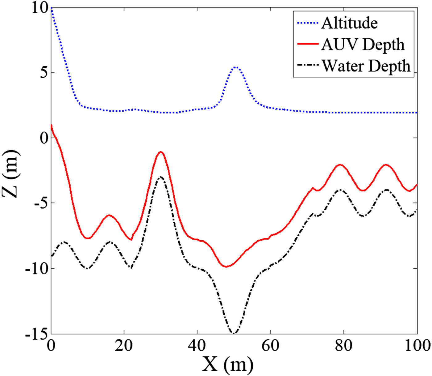
Figure 11. Bottom-following simulation at − 10 m maximum operating depth.
4. LABORATORY TRIALS
4.1. Self-Developed AUV
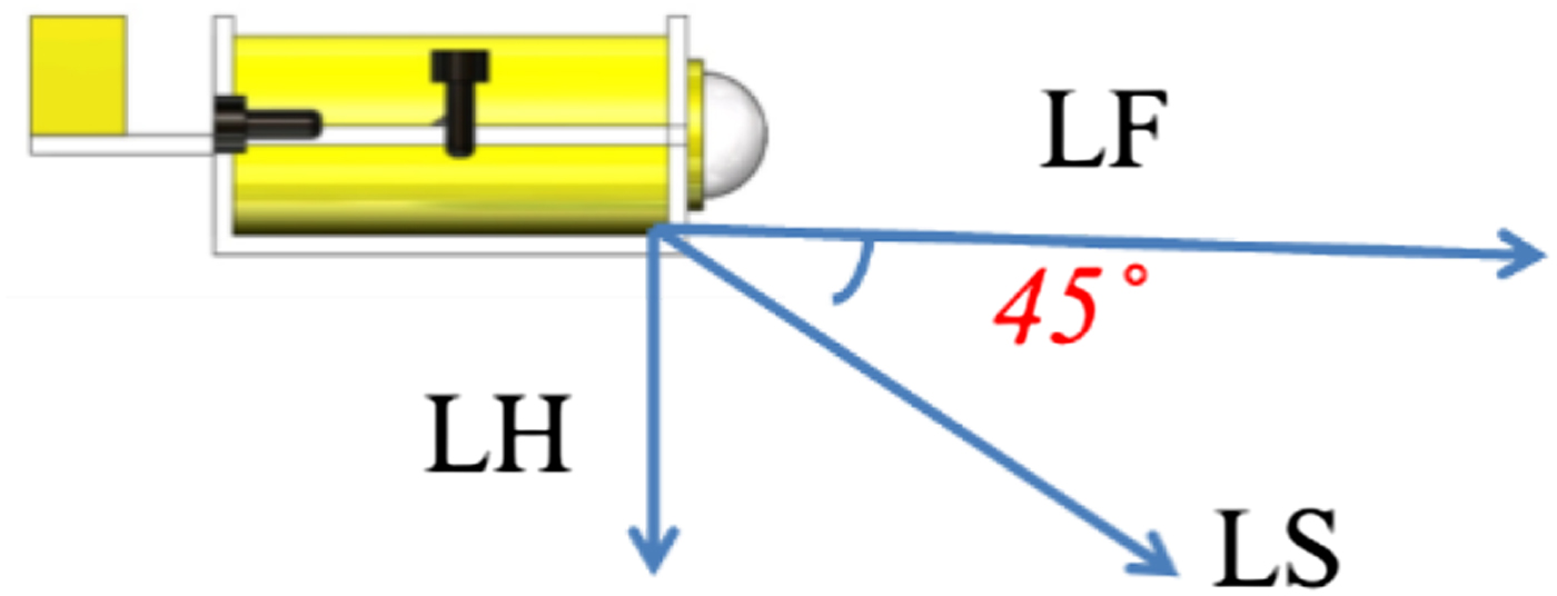
The self-developed AUV contained a power system and a control system in its waterproof hull. This consisted of four thrusters: two for surging and yawing, and the other two for heaving and rolling. It was equipped with a Doppler Velocity Log (DVL) to measure its speed, an inertial measurement unit for its attitude angles, a pressure gauge to measure its underwater depth and an underwater altimeter to measure its distance to the seabed or an obstacle. The AUV carried three altimeters for the seabed and obstacles; they were installed parallel, perpendicular, and at 45° to the hull (Figure 12), for measuring the distance to any obstacle ahead (LF), to the sea bottom directly below (LH), and to the sea bottom at 45° ahead (LS), respectively.

Figure 12. Orientations of the on board underwater altimeters.
The AUV used a CompactRIO (National Instruments) real-time controller as its primary hardware controller. The CompactRIO had Field Programmable Gate Array (FPGA) chips as processors; it was capable of parallel operations and was highly compatible with all types of sensors. The integrated LabVIEW graphical development platform enabled highly efficient customisation that allowed rapid deployment of the system. The trials were carried out in the towing tank of the Department of Systems and Naval Mechatronic Engineering, National Cheng Kung University. The tank measured  $165 \times 8 \times 4$ m; a long desk was placed at the bottom as an obstacle (Figure 13). The desk measured
  $1{\cdot}7 \times 0{\cdot}5 \times 0{\cdot}75$ m.
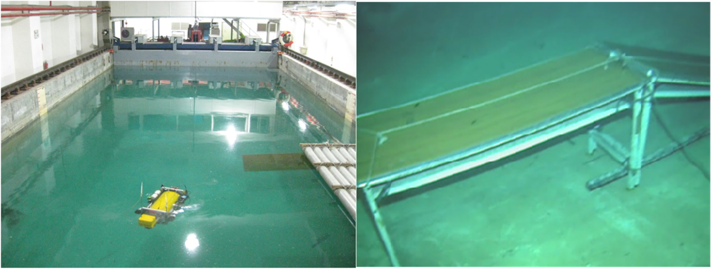
Figure 13. Towing tank and underwater obstacle.
4.2. Bathymetric measurement
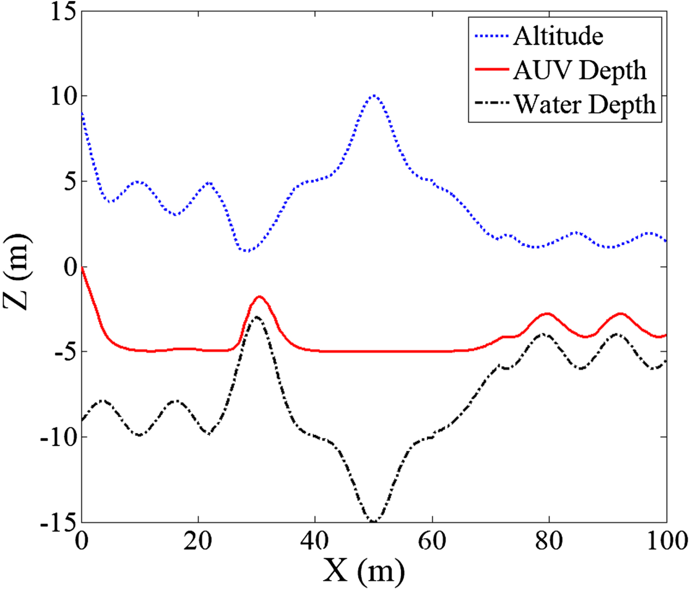
For the measurement of water depth trial, the on board pressure gauge and underwater altimeter measured the depth and altitude, from which the water depth was calculated. From the DVL, the speed of the AUV was determined to be approximately 0·2 m/sec. The measured results are shown in Figure 14, with the blue dotted line representing the measured AUV altitude, the red solid line representing the AUV depth, and the black dashed line representing the measured water depth. The height of the underwater obstacle was calculated from this data.

Figure 14. Bathymetric measurement results of the surface-cruising AUV.
4.3. Depth control trial
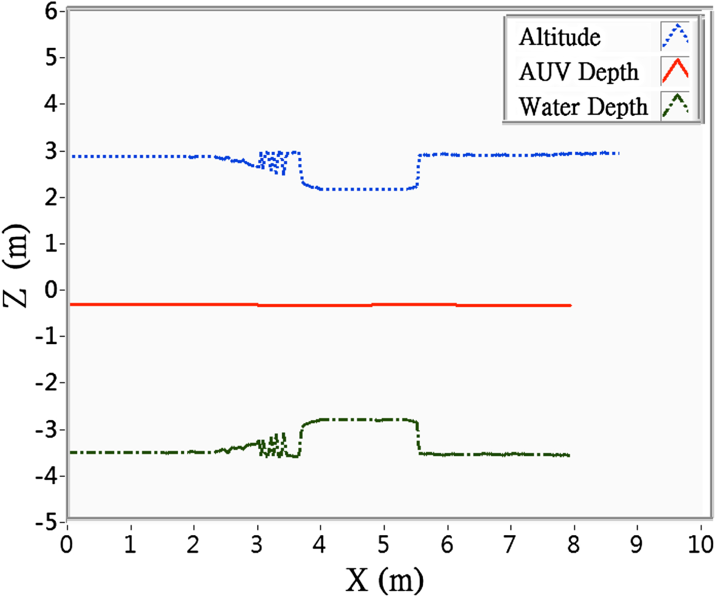
For comparison, a depth-control trial was conducted both with and without obstacle avoidance settings. The conditions were set as follows: desired depth = 1·7 m, speed = 0·25 m/sec, k az (gain value of the attractive force) = 0·5, l z (condition for the switching of attractive function) = 2 m; k rh (gain value of the repulsive force) = 0·8 and h 0 (range of the repulsive field) = 5 m. It was first conducted without obstacle avoidance settings, and the results were as shown in Figure 15. The red line shows that the AUV moved at a fixed depth throughout the course, including when it moved over the obstacle. According to the altitude data, the AUV passed the obstacle at a point only 0·7 m above the obstacle; collision would have occurred had the AUV dived slightly deeper.

Figure 15. Depth control trial at desired depth of − 1·7 m, without obstacle avoidance settings.
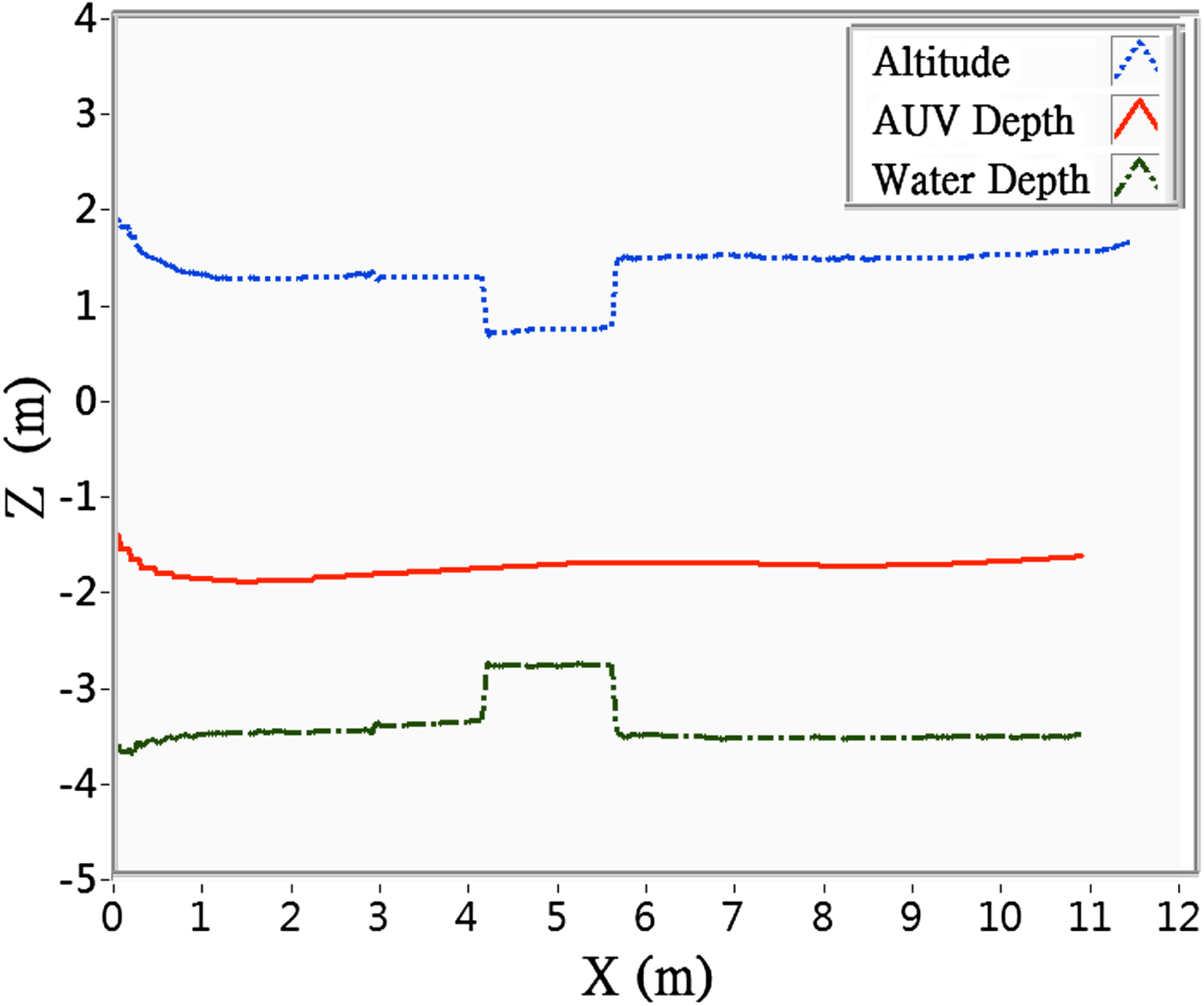
The trial was repeated with the same conditions, but with obstacle avoidance settings. The results were as shown in Figure 16, which indicates that in the beginning, the attractive force was greater than the repulsive force, hence the AUV dived down to the desired depth, until it came within range of the obstacle, at which point the decreased altitude and intensified repulsive force changed the direction of the resultant force, altered the depth-control command, and caused the AUV to veer upward to prevent collision with the obstacle, until it successfully passed the obstacle, after which the increased altitude and decreased repulsive force brought the AUV back to the desired depth.

Figure 16. Depth control trial at desired depth of − 1·7 m, with obstacle avoidance settings.
4.4. Altitude control trial
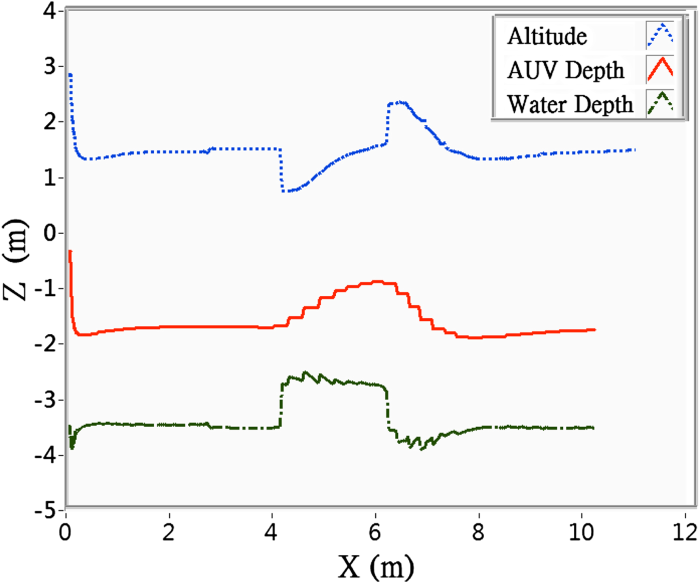
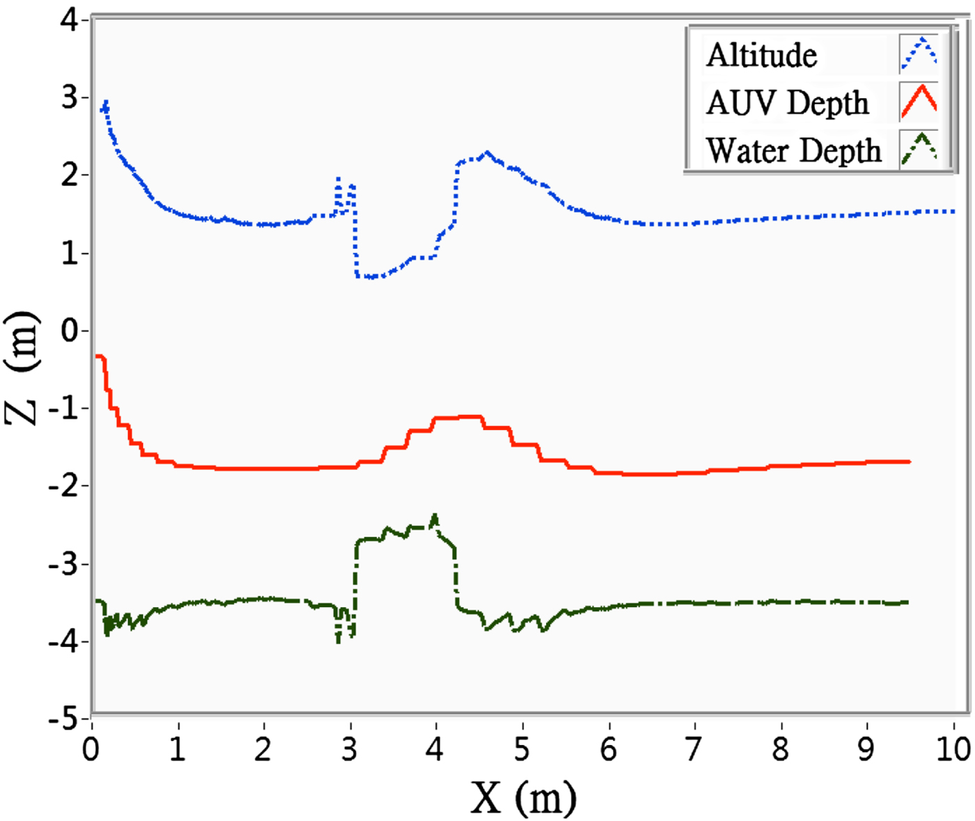
The purpose of the altitude control trial was to verify the AUV's bottom-following capability. The trial was conducted with different AUV speeds, and the results are shown in Figures 17 and 18. The maximum operating depth was set to be 5 m. At the start, the attractive force brought the AUV down to the desired altitude, after which the AUV cruised at the fixed altitude until it came within range of the obstacle; then the increased repulsive force compelled the AUV to ascend to maintain its distance from the obstacle. The results indicate that the AUV passed the altitude control trial because it was capable of following the contours of the terrain at a fixed altitude, and the trajectory of its movement maintained a constant distance from the profile of the bottom.

Figure 17. Cruising at 0·3 m/sec at desired altitude of 1·5 m.
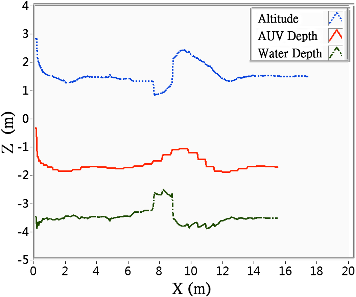
Figure 18. Cruising at 0·4 m/sec at desired altitude of 1·5 m.
5. CONCLUSION
This study proposed an APFM-based H∞ control approach for obstacle-avoidance (depth control) and bottom-following (altitude control) algorithms. The obstacle avoidance algorithm sets a desired depth to prevent the AUV from colliding with the seabed or an obstacle. Although it cannot solve the problem of local minima, which can render the AUV unable to reach its destination when the desired depth is too close to the seabed, this limitation promotes safety and ensures that the AUV will not hit the seabed. The altitude control algorithm sets a maximum operating depth to prevent the AUV from diving so far that it exceeds the limit of its structural strength when following the seabed. Simulation and laboratory trial results show that the AUV was able to meet the expected performance requirement by obeying the safety restrictions on the desired depth and altitude for all seabed terrain without any collisions. Moreover, the H∞ controller was capable of precision navigation, thus verifying the feasibility and effectiveness of the proposed combination of H∞ control and the APFM. The follow-up to this study will consider underwater signal interference, and will emphasise how to eliminate sensor noise, enhance measurement accuracy, and prevent misjudgement of signals. The results will be tested in sea trials to verify their feasibility.