Much is at stake in the 2018 state legislative elections as the Democrats battle to wrest control of key chambers from the Republicans with an eye towards redistricting after 2020. Five states clustered around the Great Lakes—Minnesota, Wisconsin, Michigan, Ohio, and Pennsylvania—as well as North Carolina and Florida—are of particular note. Collectively they account for 104 US House seats, and arguably determined the winner of the 2016 presidential election.
These states are ground zero in the “voting wars,” with all of them among the most extreme state legislative gerrymanders in the country,Footnote 1 and Wisconsin the subject of the partisan gerrymandering case Gill v. Whitford.Footnote 2 Voter identification requirements, early voting roll back, and voter list purges are election laws that have been newly implemented in many of these states.
Are these Republican gerrymanders so extreme that the Democrats will be shut out of power for another decade?Footnote 3 The forecasts presented here, made on August 27, 2018, indicate the Democrats’ prospects of winning legislative control in these states is low, with the exception of Michigan, the North Carolina Senate, and the Minnesota House. As explained in more detail in this article, the predictions presented here are in a good position to take partisan gerrymandering into account, as they predict election outcomes at the district level, and therefore take distortions in the translation of votes into seats into account. Table 1 reports the predicted change in the percentage of Democrats and also the probability each chamber will have a Democratic or Republican majority. Figures 1 and 2 display the predicted change in the percentage of Democrats by the percentage of seats they currently hold. The median prediction from the simulations is that the Democrats will pick up nine chambers in the upcoming election.
Table 1 Predicted Probability of Party Control for Chambers after the 2018 Elections
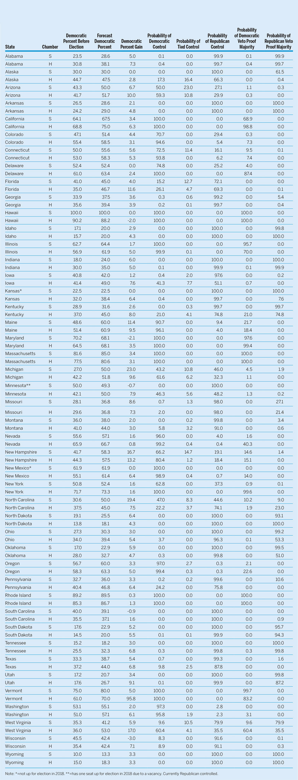
Note: *=not up for election in 2018. **=has one seat up for election in 2018 due to a vacancy. Currently Republican controlled.

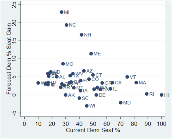
Figure 1 2018 State Senate Forecasts: Predicted Democratic Seat Gain by Current Democratic Seats

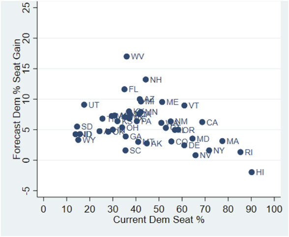
Figure 2 2018 State House Forecasts: Predicted Democratic Seat Gain by Current Democratic Seats
The Democrats have essentially no chance of taking the Ohio Senate or House, or the Pennsylvania Senate. In Wisconsin, they have just under a 10% chance of winning control of either chamber. They also have no chance of taking the Minnesota Senate, since only one of its seats is up this year (to fill a vacancy). The next tier in regards to Democratic prospects are in the Florida House and Senate, and the North Carolina and Pennsylvania Houses, which they have about a one-in-four or less chance of taking.
The remaining four chambers—the North Carolina Senate, the Minnesota House, and both chambers of Michigan—are tossups. The Minnesota House has a 46.3% chance of flipping, the North Carolina Senate has a 47.0% chance, while the Michigan Senate has a 43.2% chance, and the Michigan House has a 61.6% chance.
Democratic prospects in the Michigan Senate are surprising given they currently only hold 10 out of its 38 seats. Where will the 10 seats come from in the scenarios in which they win? The Michigan Senate is unusual in that it has four-year non-staggered terms, which are all up this year. This makes state senates much more volatile. For example, figure 1 indicates that the four state senates with the greatest amount of predicted change have all their seats up. Figure 2 shows the same predictions for state Houses.
Next, a wave of Republican incumbents initially elected in 2010—a Republican wave year—are all retiring because of term limits. Next, a large number of Republican held seats are within reach for the Democrats there, as illustrated in figure 3. In 2014, five seats were lost by the Democrats in the 45-50% range, one with 49.96% of the vote.

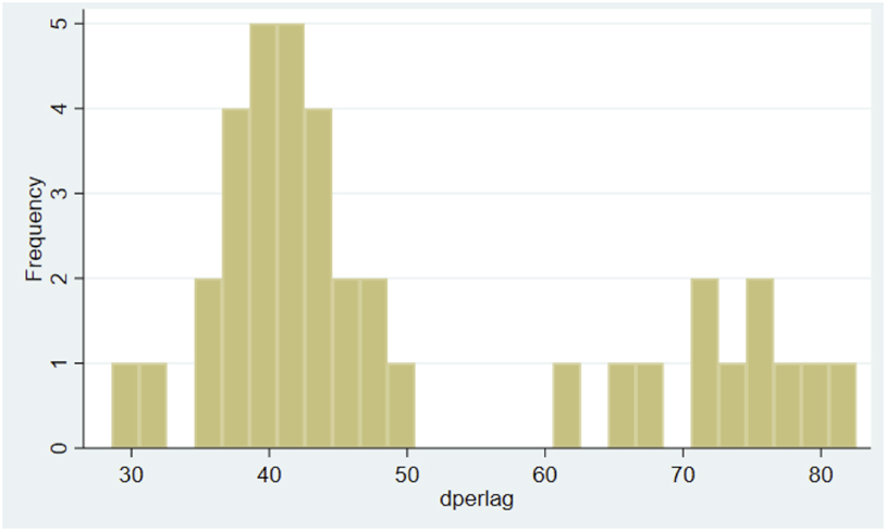
Figure 3 2014 Democratic Percent of the Vote in Michigan State Senate Races
Next, the distribution of 2014 votes is almost comical, in that they are piled around the 40% mark, which is what one would expect a party to do if they were gerrymandering a map. Historically, only one-in-eight seats flip parties if it was won with between 40 and 45% of the vote for the losing party last time, but the odds improve for the favored party in midterm years. More importantly, the number of seats within range of conceivably flipping is so high that the Democrats only have to win five of the 18 seats won with between 36 and 44% of the vote last time to take the Senate, assuming they win the five closest to 50%.
In 2010, Wisconsin and Maine were the first states since 1974 to flip from one trifecta to another—in other words, unified Democratic control of state government flipped to unified Republican control. Given that the Michigan gubernatorial race is considered a close race by many, Michigan might add to this short list this year.
In 2010, Wisconsin and Maine were the first states since 1974 to flip from one trifecta to another—in other words, unified Democratic control of state government flipped to unified Republican control. Given that the Michigan gubernatorial race is considered a close race by many, Michigan might add to this short list this year.
Also of note is the New York Senate, where a coalition of eight Democrats and the Republicans have held sway, although the Independent Democratic Caucus has disbanded and those senators say they will caucus with the Democrats. Even if we assume there is a 50% chance they will caucus with the Republicans, there is a 62.8% chance the Democrats will be in the majority in the New York Senate.
The model indicates the Iowa House has a 41.3% chance of going to the Democrats and even indicates they have a one-in-five chance of taking the Kentucky House.
ACCURACY OF 2010 AND 2014 STATE LEGISLATIVE FORECASTS
This is the third consecutive midterm for which I have made state legislative forecasts. No other quantitatively based district level forecasts for state legislative elections have been made, at least publicly.
These models performed well in both 2010 and 2014, although both forecasts understated the extent of the Republican wave in both years. In 2010, the PS forecast made on July 22, 2010 predicted that the Republicans would pick up 11 chambers, while they actually picked up 21, with 82% of chambers being correctly called (see Klarner Reference Klarner2010; Reference Klarner2011). A later forecast, made on September 18 (Klarner Reference Klarner2010b) predicted the Republicans would gain 15 chambers, and called 89% of them correctly.
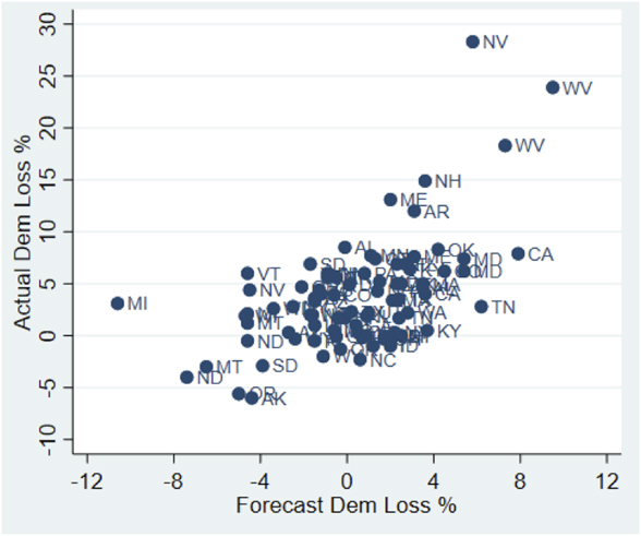
In 2014, the Republicans picked up 11 chambers, and the forecasts called 74 out of 86 chambers correctly (86.0%) (Klarner Reference Klarner2014). Humorously, an error in the simulation code identified after the election actually made the pre-election forecasts more accurate—the publicly made forecasts based on the error called 91.9% of chambers correctly. This is a noteworthy lesson about why not much should be inferred about the quality of a model based on how well it does for one prediction. The mean absolute value of error in percentage of seats held by the Democrats was 4.14%. A scatterplot of the forecast change in Democratic seats with the actual change in Democratic seats appears in figure 4, which depicts the unpublicized and less accurate forecasts.

Figure 4 2014 Forecasts Actual vs. Predicted Democratic Seat Loss
PREDICTION MODEL
Aspects of the prediction models used in 2010 (Klarner Reference Klarner2010) that are the same as the current model are as follows. State legislative elections conducted between 1968 and the present were used to assess the impact of predictor variables on election outcomes at the district level. Only regularly scheduled partisan elections conducted in even-numbered years were included in the analysis.
Predictor variables appear at three levels: district-election year, state-election year, and nation-election year.
District predictors include lagged vote share, incumbency, whether a candidate held office in the other chamber of the legislature immediately before running, and whether a candidate held legislative office in the past, but not the immediate past.
District predictors include lagged vote share, incumbency, whether a candidate held office in the other chamber of the legislature immediately before running, and whether a candidate held legislative office in the past, but not the immediate past. Other variables tracking how long incumbents have been in office were also included. Each independent variable’s lagged component also appears in the model. Controls for free-for-all multimember districts being under-contested and the level of contestation of the prior election are also included.
State level variables include a state midterm penalty (the party of the governor tends to lose seats when the governor is not up for reelection) while change in state real disposable income was omitted because tests indicated these did not bring down forecast error.
National level variables intended to capture the national partisan wave include presidential approval, a national midterm penalty variable, and change in real disposable income. The specific way these variables are coded is explained in Klarner (Reference Klarner2010).
“Drop-1 analysis” was utilized to assess whether including predictor variables reduced prediction error. In this context, “drop-1 analyses” means that the dependent variable (Democratic percentage of the vote) was turned to system missing for each election year in turn, for all state legislative elections in the country that year, coefficients were estimated using the remaining years, and forecast error in the omitted biennium was assessed.
When data were missing—most often lagged variables, missing because of redistricting—Stata’s missing data imputation algorithm was used. Drop-1 analyses indicated that prediction error goes down when missing data imputation is used, even for districts that do not have missing lagged values.
Beyond the shared attributes of the 2010 and 2018 models, numerous improvements have been made (see appendix). As explained in the appendix, these include interactions for the type of contest (such as a contest between the same winner and loser from last time), modeling the declining incumbency effect, and the addition of “supplemental” lagged variables, such as lagged values from the other chamber of the legislature when there are identical districts.
Perhaps the most noteworthy published finding about state legislative elections to date is the interaction between how much is spent on the state legislature and the electoral boost that incumbents get (Berry, Berkman, and Schneiderman Reference Berry, Berkman and Schneiderman2000). However, analyses indicated that including this interaction did not reduce prediction error, and so was removed from the model.
How the national wave is modeled has also been markedly altered. First, congressional vote intention has been added as a predictor variable, as the goal currently is to maximize forecast accuracy. Second, the four national level predictor variables have been reduced to just one variable.
Because the model presented here is a model of change, lagged independent variables for all variables are included, as was done in prior models.
A hierarchical linear model is used to estimate the impact of the predictor variables on election outcomes, and is reported in table 2. The same amount of error at higher levels is more damaging to chamber predictions, as district level predictions cancel out to an extent, so the hierarchical model allows the magnitude of these different sources of error to be computed. The findings of the model were largely consistent with theoretical expectations.
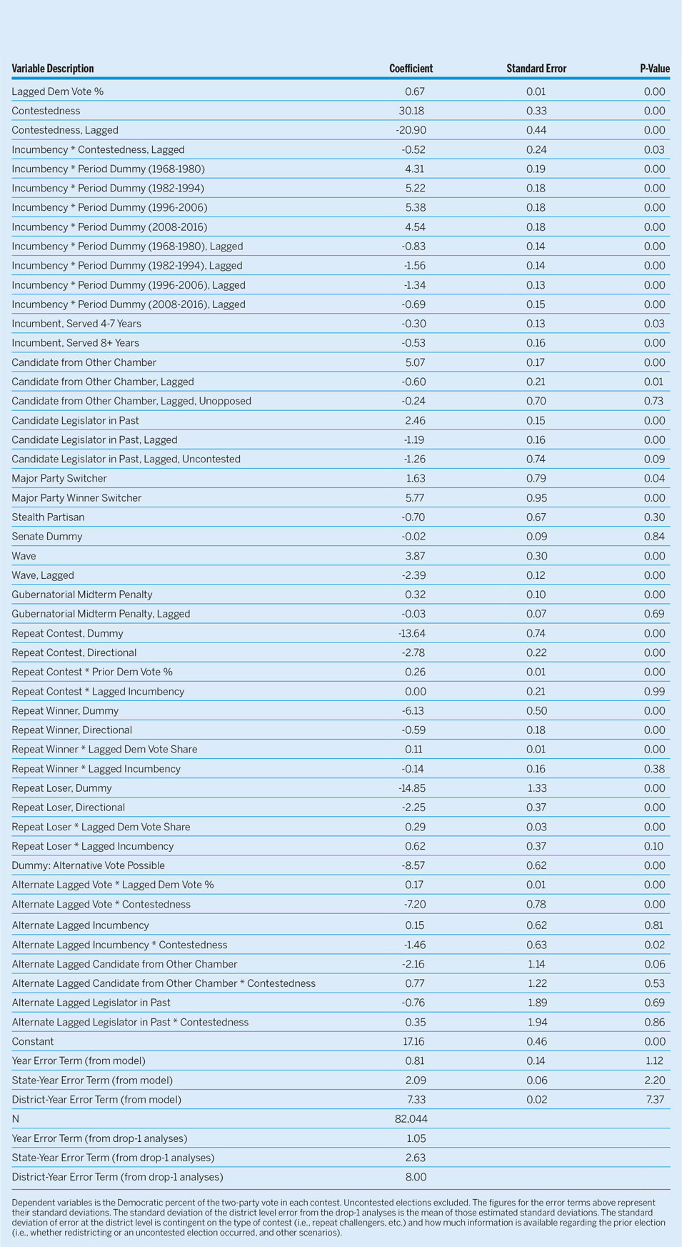
Table 2 Determinants of Democratic Vote Percentage in State Legislative Elections, 1968–2016

Dependent variables is the Democratic percent of the two-party vote in each contest. Uncontested elections excluded. The figures for the error terms above represent their standard deviations. The standard deviation of the district level error from the drop-1 analyses is the mean of those estimated standard deviations. The standard deviation of error at the district level is contingent on the type of contest (i.e., repeat challengers, etc.) and how much information is available regarding the prior election (i.e., whether redistricting or an uncontested election occurred, and other scenarios).
2018 VALUES
Candidates were collected from each state as filing deadlines passed. The last filing deadline passed on July 12, 2018, in New York, which is also a key state. Candidates were integrated into the State Legislative Election Returns database, and name matching was done to establish the identity of these candidates, after which incumbency, and other factors were also coded. When two or more candidates filed for one primary for one seat, it was assumed that incumbents would beat candidates from the other chamber, candidates from the other chamber would beat candidates with past legislative service, and candidates with past legislative service would beat candidates with no legislative service. As primaries have been conducted, 2018 incumbency scores have been altered appropriately based on primary outcomes.
SIMULATIONS
After point predictions were produced from the prediction model, simulations were conducted to see how uncertainty about each election would influence uncertainty about winning a particular chamber. The probability of ties in even seat chambers and veto-proof majorities are also displayed. For free-for-all multimember districts, an intermediate step where the number of seats a party wins based on the predicted percentage of votes that party is forecast to have in that iteration of the simulation is also conducted. This is because if the Democrats win 45% of the vote in a district with two seats, such as in the Arizona House, they may win either zero or one seat, depending on how the votes are distributed.
SUPPLEMENTARY MATERIAL
To view supplementary material for this article, please visit https://doi.org/10.1017/S1049096518001555