2.1 Undeformable bubbles

First, we consider rigid and stress-free boundary conditions on the surfaces of undeformed bubbles. These are relevant for the study of inertial migration in the cases of infinite Marangoni effect and clean surface respectively.

On the one hand, in the limit of infinite Marangoni effect, the flow at the bubble surface corresponds to that of a rigid solid that rotates with rotational velocity $\unicode[STIX]{x1D734}$ and is determined by the no-slip condition and the equilibrium of moments respectively,

These conditions are the same as those governing the case of infinitely viscous drops or solid spheres. Thus, their interactions with the liquid are identical.

On the other hand, in the case of clean bubbles, the stress-free boundary condition, which consists of vanishing tangential stresses and the impermeability condition, is applied for the case of clean bubbles, i.e.

where the surface variable $\hat{p}_{s}$ is the reduced counterpart of the impermeable surface pressure $p_{s}=\hat{p}_{s}+\boldsymbol{f}\boldsymbol{\cdot }(\boldsymbol{x}-\unicode[STIX]{x1D73A})$ that the liquid exerts on the bubble surface. These conditions are the same as those governing the case of inviscid drops. Thus, their interactions with the liquid are identical.

2.2 Deformable bubbles

Second, we consider the case of deformable bubbles, which is relevant for the study of capillary migration. In this case, the surface position is governed by the following equilibrium of stresses and the impermeability condition:

where $\unicode[STIX]{x27E6}\unicode[STIX]{x1D749}\unicode[STIX]{x27E7}=[p_{G}-\boldsymbol{f}\boldsymbol{\cdot }(\boldsymbol{x}-\unicode[STIX]{x1D73A})]{\mathcal{I}}+\hat{\unicode[STIX]{x1D749}}$ is the jump of the stress tensor and the global variable $p_{G}$ , i.e. neither domain nor surface, is the gas pressure governed by the Young–Laplace law, which depends on the volume of the bubble, ${\mathcal{V}}_{B}$ . The exterior surface differential operator $\boldsymbol{D}_{S}$ is defined by its application to a quantity $\unicode[STIX]{x1D711}$ , either scalar, vector or tensor, as

where $\unicode[STIX]{x1D6F4}$ is a surface bounded by a contour $\unicode[STIX]{x1D6E4}$ , the outer normal of which is denoted by $\boldsymbol{n}_{S}$ . The vector $\boldsymbol{n}_{S}$ is perpendicular to the contour $\unicode[STIX]{x1D6E4}$ and to the outer normal vector of the surface $\unicode[STIX]{x1D6F4}$ , $\boldsymbol{n}$ , as schematised in figure 2. It should be noted that $\boldsymbol{D}_{S}\unicode[STIX]{x1D6FE}$ includes the normal pressure proportional to the curvature and the Marangoni effect (not considered in this work), $\boldsymbol{D}_{S}\unicode[STIX]{x1D6FE}=-\unicode[STIX]{x1D6FE}\boldsymbol{n}\unicode[STIX]{x1D735}_{\!S}\boldsymbol{\cdot }\boldsymbol{n}+\unicode[STIX]{x1D735}_{\!S}\unicode[STIX]{x1D6FE}$ , with $\unicode[STIX]{x1D735}_{\!S}=({\mathcal{I}}-\boldsymbol{n}\boldsymbol{n})\boldsymbol{\cdot }\unicode[STIX]{x1D735}$ the surface gradient operator.

Figure 2. Sketch of the contour $\unicode[STIX]{x1D6E4}$ limiting the fluid surface $\unicode[STIX]{x1D6F4}$ ; $\boldsymbol{n}$ is the outer normal to the surface and $\boldsymbol{n}_{S}$ is the outer normal to the contour contained in $\unicode[STIX]{x1D6F4}$ such that $\boldsymbol{n}\boldsymbol{\cdot }\boldsymbol{n}_{S}=0$ .

Since $\unicode[STIX]{x1D6F4}_{B}$ for a bubble is a closed surface and has no contour, it can be inferred from (2.11) that the surface tension exerts no force on the bubble as a whole. Thus, the integral of (2.10a ) over $\unicode[STIX]{x1D6F4}_{B}$ leads to (2.4), and therefore (2.4) is redundant in the case of deformable bubbles.

Finally, since the domain is deformable, the volume and transverse position of the deformed bubble need to be defined,

where ${\mathcal{V}}_{B}$ is the domain occupied by the bubble.

2.3 Scaling and numerics

Equations (2.1)–(2.12) can be made dimensionless with the hydraulic diameter of the channel $d_{h}$ , the mean velocity of the flow $J$ and the viscous stress $\unicode[STIX]{x1D707}J/d_{h}$ as characteristic length, velocity and pressure respectively. Equations (2.1)–(2.12) are referred to hereafter as their dimensionless counterparts obtained by the substitution in these equations of

where the dimensionless numbers are

Typical values for water in a microchannel of diameter $d_{h}=500~\unicode[STIX]{x03BC}\text{m}$ and a flow rate of $J=0.1~\text{m}~\text{s}^{-1}$ correspond to dimensionless numbers of $Re=50$ and $Ca=1.4\times 10^{-3}$ . The dimensional domain variables can be recovered by

and the dimensional global variables by

Because of symmetry around $z=0$ , $\boldsymbol{f}$ and $\unicode[STIX]{x1D73A}$ are aligned. Thus, we choose, without loss of generality, that $\boldsymbol{e}_{y}$ is aligned with both. We define their magnitudes in this direction as $f=\boldsymbol{f}\boldsymbol{\cdot }\boldsymbol{e}_{y}$ and $\unicode[STIX]{x1D700}=\unicode[STIX]{x1D73A}\boldsymbol{\cdot }\boldsymbol{e}_{y}$ respectively. In addition, also due to symmetry, the rotation takes place within the plane $x$ – $y$ , and we define its magnitude as $\unicode[STIX]{x1D734}=\unicode[STIX]{x1D6FA}\boldsymbol{e}_{z}$ .

In the numerical simulations, the relations between $\unicode[STIX]{x0394}p$ and $J$ , $\unicode[STIX]{x1D700}$ and $f$ as well as, in the case of deformable bubbles, $p_{G}$ and ${\mathcal{V}}_{B}$ , need to be parametrised. For this purpose, we impose $J$ , $\unicode[STIX]{x1D700}$ and ${\mathcal{V}}_{B}$ , whereas $\unicode[STIX]{x0394}p$ , $f$ and $p_{G}$ are solved. This particular choice is because we make the system of equations dimensionless with $J$ , the function $\unicode[STIX]{x1D700}=\unicode[STIX]{x1D700}(f)$ might be multivalued, whereas the inverse, $f=f(\unicode[STIX]{x1D700})$ , is not, and the size of the bubble ${\mathcal{V}}_{B}$ together with its transverse position $\unicode[STIX]{x1D73A}$ fix the domain ${\mathcal{V}}$ . Although for deformable bubbles the domain deforms, it is numerically convenient to use an initial domain as similar as possible to the deformed one. Furthermore, it is the case for small $Ca$ values for which the bubble is spherical and $Ca$ can be increased using continuation methods, enhancing convergence.

We consider that the bubble is undeformable for strictly $Ca=0$ , and deformable for $Ca\neq 0$ .

In the case of undeformable bubbles, the variables used in the simulations are the domain variables $\hat{p}$ and $\boldsymbol{v}$ , the surface variable $\hat{p}_{s}$ (only for a stress-free interface) and the global variables $f$ , $V$ , $\unicode[STIX]{x0394}p$ and $\unicode[STIX]{x1D6FA}$ (only for a rigid interface). These variables are governed by (2.1)–(2.6) and either (2.8) or (2.9), for bubbles with rigid or stress-free interfaces respectively.

In the case of deformable bubbles, the variables are the domain variables $\hat{p}$ and $\boldsymbol{v}$ , and the global variables $p_{G}$ , $f$ , $V$ and $\unicode[STIX]{x0394}p$ . These variables are governed by (2.1), (2.2), (2.3), (2.5), (2.6) and (2.10). The deformation of the bubble is handled using the arbitrary Lagrangian–Eulerian (ALE) method (Donea, Giuliani & Halleux Reference Donea, Giuliani and Halleux1982) together with the volume and transverse position definitions (2.12).

The aforementioned systems of equations are solved using the finite element method (FEM). The equations are implemented in weak form using the software COMSOL and the moving mesh module that implements the ALE method. Details of the definition and discretisation using the FEM of the surface operators such as $\boldsymbol{D}_{S}$ and $\unicode[STIX]{x1D735}_{\!S}$ are given in appendix A.

We have validated the implementation of the previous equations by comparing the equilibrium position of a particle with diameter $d=0.305$ for $Re=0.196$ , in the absence of body force, obtained by other authors both numerically and experimentally; see figure 2 in Yang et al. (Reference Yang, Wang, Joseph, Hu, Pan and Glowinski2005). We benefit from the symmetry with respect to the $z=0$ plane to reduce by a factor of $2$ the domain size, although the computational time – which remains within the range of a few minutes (1–3 min) for one solution on a regular desk computer – is not limiting in the computations reported here. We have also carefully checked the convergence of a tetrahedral mesh with hexahedral elements on the bubble surface. Symmetric meshes with respect to the $x=0$ plane have been found to increase the accuracy on the solution.

3.1 Inertial migration

Straight channels represent a particular geometry in which a constant flow does not depend on the Reynolds number provided that no turbulence develops, and it corresponds to the purely creeping flow which is reversible. However, the presence of the bubble modifies the flow structure in such a manner that inertial forces come into play and, thus, break the reversibility of the flow. In this case, the bubble experiences a transverse force of inertial origin even for small but finite inertial forces (Segré & Silberberg Reference Segré and Silberberg1962). This motivates an expansion of the system of equations (2.1)–(2.6) and either (2.8) or (2.9) for small Reynolds number as $\unicode[STIX]{x1D713}=\sum _{j=0}^{\infty }Re^{j}\unicode[STIX]{x1D713}_{j}$ , where $\unicode[STIX]{x1D713}$ represents any of the dependent variables $\hat{p}$ , $\boldsymbol{v}$ , $\boldsymbol{f}$ , $V$ , $\unicode[STIX]{x0394}p$ and either $\hat{p}_{s}$ or $\unicode[STIX]{x1D734}$ , which yields (Cox & Brenner Reference Cox and Brenner1968), up to first order,

with vanishing body force in the axial direction (2.2),

together with the linearisation of the velocity at the walls (2.3),

of the equilibrium equations for the bubble (2.4),

of the periodic conditions (2.5),

and of the mean flow (2.6),

The linearisation of the boundary conditions on the bubble surface is

for a rigid interface, or

for a stress-free interface. It should be noted that the migration force can be alternatively computed using the reciprocal theorem, as performed by Ho & Leal (Reference Ho and Leal1974) in the limit of $Re\ll 1$ and $d\ll 1$ .

The solution of the system (3.1)–(3.8) for the inertial migration force, bubble velocity, pressure drop and rotational velocity (only applicable in the case of a rigid interface) is of the form, truncated at $O(Re^{2})$ ,

where the removed terms have been found numerically to be vanishing, i.e. $f_{0}=V_{1}=\unicode[STIX]{x1D6FD}_{1}=\unicode[STIX]{x1D6FA}_{1}=0$ , as can be inferred from the symmetries and reversibilities of the flow shown in appendix B. Consequently, the balanced body force comes from the first-order solution, whereas the velocity and pressure correction factor and rotational velocity come from the zeroth-order solution. Results on the inertial migration force $f$ have been recently reported (Yang et al. Reference Yang, Wang, Joseph, Hu, Pan and Glowinski2005; Di Carlo et al. Reference Di Carlo, Edd, Humphry, Stone and Toner2009; Stan et al. Reference Stan, Guglielmini, Ellerbee, Caviezel, Stone and Whitesides2011). We contribute with the systematic study of the effect of the bubble size $d$ on $f$ in addition to the functions $V(\unicode[STIX]{x1D700},d)$ , $\unicode[STIX]{x1D6FD}(\unicode[STIX]{x1D700},d)$ and $\unicode[STIX]{x1D6FA}(\unicode[STIX]{x1D700},d)$ (if applicable).

Figure 4. The effect of the transverse position $\unicode[STIX]{x1D700}$ of a bubble with a rigid interface and size $d=0.4$ in the pure linear inertial regime on the (a) balanced body force, (b) bubble velocity, (c) pressure correction factor and (d) rotational velocity.

In figure 4, we depict the solution (3.9) for a representative bubble of size $d=0.4$ in the small-Reynolds-number limit for values of the transverse position within the geometrically feasible range $-\unicode[STIX]{x1D700}_{\ast }<\unicode[STIX]{x1D700}<\unicode[STIX]{x1D700}_{\ast }$ , where $\unicode[STIX]{x1D700}_{\ast }=(1-d)/2$ corresponds to the position of a spherical bubble touching the wall. In figure 4(a), we can observe the existence of multiple equilibrium positions of the bubble for a range of values of the balanced body force $f$ . This multiplicity of solutions is lost for sufficiently large values of the balanced body force and for bubbles closer to the wall. In particular, for the case of a neutral bubble, i.e. no body force, $f=0$ , there exist typically three equilibrium solutions, whose stability is determined by the slope $\unicode[STIX]{x2202}_{\unicode[STIX]{x1D700}}f$ , two of which are stable, denoted by (i) and (iii), whose attraction ranges are separated by the unstable one (ii). It is represented by the line decorated with arrows, indicating the transverse motion of a bubble when located out of the equilibrium position. In addition, this can be observed by turning the force on towards negative values but moderate ones, so that multiple solutions still exist, as exemplified for $f/Re=-0.15$ in figure 4(a). In effect, this results in a positive force exerted on the bubble, and, therefore, bubbles at stable positions, namely in positions (i) and (iii), are shifted upward towards positions (iv) and (vi), i.e. in the same direction as the force exerted on the bubble, namely to the right in figure 4(a). Unstable bubbles, namely at position (ii), are shifted in the opposite direction towards (v), revealing the unstable character of this position. Analogous reasons show that the positions (iv)–(vi) show the same character as (i)–(iii). Once the equilibrium position for a given body force $f$ is known, one can obtain from figure 4(b–d) the values of $V$ , $\unicode[STIX]{x0394}p$ and $\unicode[STIX]{x1D6FA}$ . In effect, at the centre of the channel, i.e. $\unicode[STIX]{x1D700}=0$ , the bubble velocity is maximal, the pressure drop is minimal and the rotational velocity reverses orientation. Given the symmetries of the functions in (3.9) with respect to the position of the bubble, it is sufficient to explain them only for positive transverse positions, $\unicode[STIX]{x1D700}\geqslant 0$ . One can note the odd symmetry of the balance body force for which any condition has an equivalent for the opposite position, as illustrated in figure 4(a) by the positions ( $\text{iv}^{\prime }$ ), ( $\text{v}^{\prime }$ ), ( $\text{vi}^{\prime }$ ) in the case of moderate and positive force, $f/Re=+0.15$ .

Figure 5. Streamlines $\boldsymbol{v}_{0}$ , and colourmap for the pressure field, $\hat{p}_{0}-x\unicode[STIX]{x1D6E5}_{x}p_{P}$ , in the leading-order creeping regime at the symmetry plane $z=0$ for neutral bubbles $f/Re=0$ with rigid interface and size $d=0.4$ . The labels correspond to points in figure 4(a).

The flow pattern and pressure field allow us to rationalise expressions (3.9). In particular, the zeroth-order solutions, depicted in figure 5, reveal the antisymmetry and reversibility of the creeping flow. The positions of the bubbles in figure 5 correspond to the points in figure 4 labelled with the same roman number. It can be observed that points (i) and (iii) correspond to upside-down flip due to the symmetry around the plane $y=0$ .

Figure 6. Streamlines in the leading-order creeping regime, $\boldsymbol{v}_{0}$ , and colourmap for the perturbation pressure field in the pure linear inertial regime, $\hat{p}_{1}$ , at the symmetry plane $z=0$ for (i–iii) neutral $f/Re=0$ and (iv–vi) non-neutral $f/Re=-0.15$ bubbles with rigid interface and size $d=0.4$ . The labels correspond to points in figure 4(a).

The behaviour of inertial migration can be explained with the help of the zeroth-order flow pattern and the first-order correction of the pressure field shown in figure 6. In this latter case, the flow is symmetric and antireversible, as explained in appendix B, which forces the first-order bubble velocity, pressure drop and rotational velocity to vanish, whereas the first-order balanced body force can be non-zero. In figure 4(a), points (i)–(iii) correspond to neutral bubbles, which means that the underpressure and overpressure zones observed in figure 6(i)–(iii) should counterbalance one another. To understand the stability of neutral bubbles, we plot in figure 6(iv)–(vi) the counterparts for a moderate negative body force, as in figure 4(a). The displacement of bubbles from positions (i) to (iv) and (iii) to (vi) respectively leads to a variation of the net force exerted on the bubble in the opposite direction to the displacement. In both cases, an increase of the underpressure and a decrease of the overpressure can be seen, which provides the migration force balancing the body force. In contrast, the displacement from (ii) to (iv) leads to a variation in this force in the same direction as the displacement, due to an underpressure from this side, making this position unstable, as inferred in figure 4(a).

Figure 7. The effect of the transverse position $\unicode[STIX]{x1D700}$ and the size $d$ of a bubble with a rigid interface in the pure linear inertial regime on the (a) balanced body force, (b) bubble velocity, (c) pressure correction factor and (d) rotational velocity. Not explored,

; $\unicode[STIX]{x1D700}=\unicode[STIX]{x1D700}_{\ast }$ , ——; stability transition, - - - -.

In figure 7, we plot the global variables $f$ , $V$ , $\unicode[STIX]{x1D6FD}$ and $\unicode[STIX]{x1D6FA}$ (3.9) describing the bubble dynamics with a rigid interface (3.7) in the pure linear inertial regime, see figure 3, as a function of the diameter and the position of the bubble. Because of numerical limitations, we only computed solutions within the ranges $0.1\leqslant d\leqslant 0.9$ and $0\leqslant \unicode[STIX]{x1D700}\leqslant 0.95\unicode[STIX]{x1D700}_{\ast }$ . We observe in figure 7(a) that neutral bubbles, $f=0$ , with diameter $d\lesssim 0.73$ are unstable at the centred position, as revealed by the positive value of $\unicode[STIX]{x2202}_{\unicode[STIX]{x1D700}}f/Re>0$ . We also observe that centred bubbles with diameter $d\approx 0.3$ are the most unstable and that the equilibrium position moves away from the centre as the size diminishes. The transition between unstable and stable positions is depicted with black-dashed lines, which correspond to the local extremum of figure 4(a), illustrated with

for $d=0.4$ . One can note the imperfect pitchfork bifurcation of the transverse position with $d$ as the parameter and $f$ as the imperfection, which contains information on the stability of the centred branch. Some relevant conditions exhibiting these features are depicted in figure 4(a); see points (ii) and (iii). In figure 7(b), we can numerically observe that small bubbles follow the Poiseuille flow, $V_{P}=2(1-4\unicode[STIX]{x1D700}^{2})$ . Proximity of the bubble to the wall, either because of larger bubble size or due to transverse position, turns out to make the bubble travel more slowly. The rotational bubble velocity corresponds to the rotational velocity of the Poiseuille flow (half of the vorticity), $\unicode[STIX]{x1D6FA}=-\unicode[STIX]{x2202}_{\unicode[STIX]{x1D700}}V_{P}/2=8\unicode[STIX]{x1D700}$ , as shown in figure 7(d). In fact, bubbles, also with large size, tend to assure continuity of the liquid at the rigid interface of the bubble, with a velocity very similar to the average over the bubble surface of the Poiseuille velocity, $V\approx \unicode[STIX]{x1D6F4}_{B}^{-1}\int _{\unicode[STIX]{x1D6F4}_{B}}2[1-4(y^{2}+z^{2})]\,\text{d}\unicode[STIX]{x1D6F4}$ , even for large bubble size as plotted in figure 7(b) with coloured thin dashed lines. The rotational velocity, depicted in figure 7(d), also reduces due to the effect of the wall. A bubble with rigid interface behaves like a plug since for large size the pressure drop increases with the bubble size, as shown in figure 7(c).

Figure 8. The effect of the transverse position $\unicode[STIX]{x1D700}$ and the size $d$ of a bubble with a stress-free interface in the pure linear inertial regime on the (a) balanced body force, (b) bubble velocity and (c) pressure correction factor. Not explored,

; $\unicode[STIX]{x1D700}=\unicode[STIX]{x1D700}_{\ast }$ , ——; stability transition, - - - -.

In figure 8, we depict the influence of the bubble size on the dynamics of the bubble with a stress-free interface (3.8). In figure 8(a), we plot the body force $f$ , related to the migration force by (2.4). Analogous behaviour to the bubble with rigid interface is observed. In this case, the transition of stability for centred bubbles takes place at around $d\approx 0.85$ , and the most unstable centred bubbles are those with diameter $d\approx 0.63$ . The range of position for which bubbles with stress-free interface are unstable is larger than for bubbles with rigid interface. We observe that there exists a range of bubble size $0.35\lesssim d\lesssim 0.83$ for which bubbles are touching the wall, i.e. in practice for $\unicode[STIX]{x1D700}>0.95\unicode[STIX]{x1D700}_{\ast }$ . In figure 8(b), we can again numerically observe that small bubbles follow the Poiseuille flow $V_{P}$ and, in the absence of body force, the bubble migrates to the position at which it travels at the mean flow velocity, i.e. $V=V_{P}=1$ at $\unicode[STIX]{x1D700}=\sqrt{2}/4$ . Proximity of the bubble to the wall, either because of bubble size or due to transverse position, turns out to make the bubble travel more slowly. In figure 8(c), we observe the pressure correction factor due to the presence of the bubble. We highlight the conditions for which the pressure correction factor vanishes, i.e. the transition to the parametrical region where the presence of a bubble reduces the pressure drop. Unfortunately, these positions are all unstable, and stable bubbles in the pure linear inertial regime always increase the pressure drop.

For the sake of completeness, polynomial fittings of the functions (3.9) are given in appendix C for both rigid and stress-free interfaces.

For sufficiently large $Re$ , the solution (3.9) is no longer valid, as we observe in figure 9, where the balanced body force is depicted versus the transverse position for various Reynolds numbers for a bubble with diameter $d=0.4$ in the case of bubbles with rigid interface and the pure nonlinear inertial regime. The behaviour remains qualitatively similar to the pure linear inertial migration.

Figure 9. The influence of the Reynolds number on the balanced body force for bubbles of size $d=0.4$ with a rigid interface in the pure nonlinear inertial regime.

The validity of the pure linear inertial regime, $Re<Re_{\ast }$ , can be quantified as follows with two different criteria depicted in figure 10. On the one hand, in figure 10(a,c), we plot the influence of the Reynolds number and the bubble size on the stability of the centred position given by $\unicode[STIX]{x2202}_{\unicode[STIX]{x1D700}}f/Re|_{\unicode[STIX]{x1D700}=0}$ . It can be observed that the range of validity of small $Re$ is slightly larger for bubbles with stress-free interface than with rigid one. The variation of the slope is referred to the one of the linear regime and normalised by the value of the latter for bubbles of size $d=0.3$ and $d=0.63$ for bubbles with rigid or stress-free interfaces respectively. These values correspond to local maxima of $\unicode[STIX]{x2202}_{\unicode[STIX]{x1D700}}f/Re|_{\unicode[STIX]{x1D700}=0}$ versus $d$ . On the other hand, the equilibrium position of neutral bubbles is modified. In figure 10(b,d), we plot the influence of the Reynolds number on the equilibrium position of a neutral bubble of certain size, i.e. in the absence of body force. The nonlinear effect of the inertia turns out to be destabilising, in general, either concerning the stability of the equilibrium, whose slope, $\unicode[STIX]{x2202}_{\unicode[STIX]{x1D700}}f$ , increases, or concerning the neutral bubble position, which is shifted away from the centre.

Figure 10. The influence of the Reynolds number and the size of a bubble with (a,b) a rigid or (c,d) a stress-free interface in pure nonlinear inertial regime for bubbles on (a,c) the slope of the balanced migration force exerted on centred bubbles with respect to the transverse position (– – – – –, stability transition) and (b,d) the equilibrium position of neutral bubbles. Not explored,

; validity criterion $Re<Re_{\ast }(d)$ with $\cdots \cdots$  5 % error, – ⋅ – ⋅ – 2 % error and - - - - 1 % error.

3.2 Capillary migration

Migration forces may also arise if the bubble is deformable. In this case, the reversibility of the creeping flow is broken due to the antisymmetric deformation of the bubble. Indeed, the bubble deforms differently on its front and rear sides, due to pressure gradients of the creeping flow along the bubble surface. In figure 11, the deformation of the bubble due to the viscous and pressure forces exerted on its surface in the pure nonlinear capillary regime is depicted for given values of the transverse position and bubble size, whereas $Ca$ is varied. In particular, it can be observed that the overpressure (underpressure) for small $Ca$ deforms the bubble, locally decreasing (increasing) the curvature of the bubble surface, and the bubble deforms, as shown in figure 11. The capillary migration force exerted on the bubble surface always points towards the centre of the channel, as inferred from the dominant effect of the overpressure in figure 11(b,c).

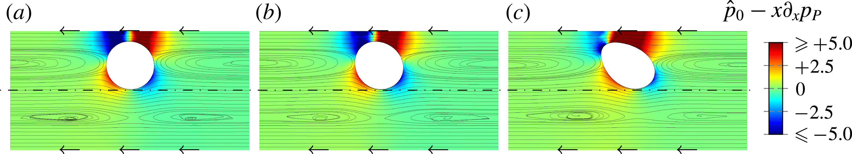
Figure 11. Streamlines, $\boldsymbol{v}$ , and colourmap for the pressure field, $\hat{p}-x\unicode[STIX]{x2202}_{x}p_{P}$ , in the pure nonlinear capillary regime at the symmetry plane $z=0$ with bubble size $d=0.4$ centred at $\unicode[STIX]{x1D700}=0.7\unicode[STIX]{x1D700}_{\ast }$ and capillary numbers (a) $Ca=1/64$ , (b) $Ca=1/16$ and (c) $Ca=1/4$ .

The analogous role of $Ca$ in the pure capillary regimes, as compared with $Re$ in the pure inertial regimes, motivates an expansion of the system of equations (2.1)–(2.3), (2.5), (2.6) and (2.10) as $\unicode[STIX]{x1D713}=\sum _{j=0}^{\infty }Ca^{j}\unicode[STIX]{x1D713}_{j}$ , where $\unicode[STIX]{x1D713}$ represents any of the dependent variables $\hat{p}$ , $\boldsymbol{v}$ , $\boldsymbol{f}$ , $V$ or $\unicode[STIX]{x0394}p$ . In addition, the fact that for $Ca=0$ the dimensional pressure of the gas scales as $\unicode[STIX]{x1D6FE}/d$ motivates an expansion of the pressure of the gas, $p_{G}$ , starting from the minus first-order term, i.e. $p_{G}=\sum _{j=-1}^{\infty }Ca^{j}p_{Gj}$ .

The linearisation of the surface of the bubble $\unicode[STIX]{x1D6F4}_{B}$ is written as the displacement of the unperturbed surface $\unicode[STIX]{x1D6F4}_{B_{0}}$ in the normal direction by an infinitesimal amount $\unicode[STIX]{x1D6FF}$ , i.e. $\boldsymbol{x}=\boldsymbol{x}_{0}+\boldsymbol{n}\unicode[STIX]{x1D6FF}$ , where $\boldsymbol{x}_{0}\in \unicode[STIX]{x1D6F4}_{B_{0}}$ and $\boldsymbol{x}\in \unicode[STIX]{x1D6F4}_{B}$ . The fact that $\unicode[STIX]{x1D6FF}=0$ for $Ca=0$ motivates that its expansion starts from the first order, $\unicode[STIX]{x1D6FF}=\sum _{j=1}^{\infty }Ca^{j}\unicode[STIX]{x1D6FF}_{j}$ . In figure 12(a), we depict the unperturbed domain ${\mathcal{V}}_{0}$ with its bubble surface $\unicode[STIX]{x1D6F4}_{B_{0}}$ and their perturbed counterparts ${\mathcal{V}}$ and $\unicode[STIX]{x1D6F4}_{B}$ respectively. In figure 12(b), we schematise an infinitesimal portion of the perturbation volume, denoted by $\unicode[STIX]{x1D6F4}_{B_{0}}\unicode[STIX]{x1D6FF}$ , which is generated by the displacement $\unicode[STIX]{x1D6FF}\boldsymbol{n}_{0}$ of an infinitesimal surface lying on the unperturbed one, $\text{d}\unicode[STIX]{x1D6F4}_{B_{0}}$ , where subindex $0$ represents evaluation at the unperturbed surface. This volume is a truncated cone bounded by the infinitesimal surfaces lying on the unperturbed and perturbed surfaces, and the generatrix with outer normal vector $\unicode[STIX]{x1D6FF}\boldsymbol{n}_{S0}$ . The perturbed volume ${\mathcal{V}}$ is the junction of the unperturbed and perturbation ones, i.e. ${\mathcal{V}}\equiv {\mathcal{V}}_{0}\cup \unicode[STIX]{x1D6F4}_{B_{0}}\unicode[STIX]{x1D6FF}$ .

Figure 12. (a) Sketch of the unperturbed volume ${\mathcal{V}}_{0}$ bounded by the unperturbed surface $\unicode[STIX]{x1D6F4}_{B_{0}}$ and their perturbed counterparts ${\mathcal{V}}$ and $\unicode[STIX]{x1D6F4}_{B}$ . (b) Infinitesimal portion of the perturbation volume $\text{d}\unicode[STIX]{x1D6F4}_{B_{0}}\unicode[STIX]{x1D6FF}$ and its bounding boundaries. Subindex $0$ represents evaluation at the unperturbed surface, whereas the lack of it represents evaluation at the perturbed one.

Then, the linearisation of the Navier–Stokes equations (2.1), neglecting inertia, $Re=0$ , is written as

at the unperturbed volume ${\mathcal{V}}_{0}$ and, using the Stokes theorem and rearranging terms,

at the perturbation volume $\unicode[STIX]{x1D6F4}_{B_{0}}\unicode[STIX]{x1D6FF}$ , where $\boldsymbol{D}_{S}\boldsymbol{\cdot }\unicode[STIX]{x1D6FF}\boldsymbol{v}$ and $\boldsymbol{D}_{S}\boldsymbol{\cdot }\unicode[STIX]{x1D6FF}\hat{\unicode[STIX]{x1D749}}$ represent the terms due to the fluxes though the generatrix, which have been rewritten using (2.11). It is also necessary to consider the identity $\unicode[STIX]{x1D735}[p_{G}-\boldsymbol{f}\boldsymbol{\cdot }(\boldsymbol{x}-\unicode[STIX]{x1D73A})]+\boldsymbol{f}=0$ , which always holds. Its evaluation at the perturbation volume $\unicode[STIX]{x1D6F4}_{B_{0}}\unicode[STIX]{x1D6FF}$ is rearranged, using the Stokes theorem, as

Equations (2.2), (2.3), (2.5) and (2.6) are linearised as in the inertial migration case, (3.2), (3.3), (3.5) and (3.6), because the rest of the boundaries do not deform. However, the linearisation of the Young–Laplace equation (2.10a ) is applied on the perturbed boundary $\unicode[STIX]{x1D6F4}_{B}$ , and can be written on the unperturbed boundary with the help of (3.11) and (3.12) as well as with (D 4) for the surface tension term, whose details are given in appendix D, as

for minus first order and

for zeroth and first order, where $\boldsymbol{D}_{S}1$ is the surface mean curvature vector and $\unicode[STIX]{x1D717}_{j}=\unicode[STIX]{x1D735}_{\!S}\boldsymbol{\cdot }(\unicode[STIX]{x1D6FF}_{j}\boldsymbol{n})$ is the surface dilatation at $j$ th order. It should be noted that $\unicode[STIX]{x27E6}\unicode[STIX]{x1D749}_{-1}\unicode[STIX]{x27E7}=p_{G-1}{\mathcal{I}}$ . Similarly, the linearisation of the impermeability condition on the bubble surface (2.10b ) is written, using (3.11), as

The linearisation of the volume and the transverse position definitions (2.12) is written, with the help of the Reynolds transport theorem, as

where ${\mathcal{V}}_{B_{0}}$ is the domain occupied by the unperturbed bubble, and its perturbation

Since $p_{G-1}$ is a global variable, the solution of (3.13) and (3.16) is a sphere of volume ${\mathcal{V}}_{B}$ and at a position $\unicode[STIX]{x1D73A}$ ,

whose surface dilatation is $\unicode[STIX]{x1D717}_{j}=-4\unicode[STIX]{x1D6FF}_{j}/d$ .

Solutions of the system (3.2), (3.3), (3.5), (3.6), (3.10), (3.14), (3.15) and (3.17) for the balanced body force, bubble velocity and pressure correction factor are of the form, truncated at $O(Ca^{2})$ ,

where the removed terms have been found numerically to be vanishing, i.e. $f_{0}=V_{1}=\unicode[STIX]{x1D6FD}_{1}=0$ , as can be inferred from the symmetries and reversibilities of the flow. It can be observed that the capillary migration force comes from the first-order solution, whereas the velocity and pressure drop come from the leading-order creeping regime, analogous to the inertial migration case. Furthermore, the sum of the capillary terms of (3.14a ) only has a normal component, i.e.

Thus, the zeroth order of the capillary regime is exactly the same as the zeroth order of the inertial regime with stress-free interface, since one can identify the capillary terms of the former as the reduced counterpart of the impermeable surface pressure $\hat{p}_{s}$ ,

In figure 13, we depict solutions of the pure nonlinear capillary flow for several values of $Ca$ and its linear limit to which the nonlinear solution converges when $Ca$ is sufficiently small, $Ca<Ca_{\ast }$ ; see figure 3. The dependence of the balanced body force, the velocity and the pressure drop on the transverse position is shown for a given bubble size. It can be observed that the capillary migration is always stabilising since $\unicode[STIX]{x2202}_{\unicode[STIX]{x1D700}}f<0$ , as shown in figure 13(a). We also observe that large deformations reduce bubble migration, increase the bubble velocity and reduce the associated pressure drop. In figure 13(b) and (c), the limit of the pure linear capillary regime reproduces the bubble velocity and the pressure drop for stress-free bubbles in zeroth-order creeping flow, $V_{0}$ and $\unicode[STIX]{x0394}p_{0}$ , the latter being negative for some conditions. Remarkably, in this case, the bubble is stable for these conditions and, therefore, the presence of a deformable bubble may reduce the pressure drop.

Figure 13. The effect of the deformability of a bubble with size $d=0.4$ and the transverse position in the pure nonlinear capillary regime on the (a) balanced body force, (b) bubble velocity and (c) pressure correction factor.

The dependence of the balanced body force on the bubble size $d$ and transverse position $\unicode[STIX]{x1D700}$ in the pure linear capillary regime is depicted in figure 14. Bubbles experience a stronger repulsion from the wall as they become closer to it either because of their size or because of their position. The velocity and pressure correction factors are the same as in the pure linear inertial regime with stress-free boundary conditions (figure 8 b,c). In effect, positions that reduce the pressure drop with respect to that of Poiseuille flow are stable in the pure linear capillary regime.

Figure 14. The effect of the transverse position $\unicode[STIX]{x1D700}$ and the size $d$ of a bubble in the pure linear capillary regime on the balanced body force. Not explored,

; $\unicode[STIX]{x1D700}=\unicode[STIX]{x1D700}_{\ast }$ , ——.

For the sake of completeness, polynomial fitting of the function $f_{1}$ (3.19) is given in appendix C, table 5.

The validity of the pure linear capillary regime is lost either for not sufficiently small capillary numbers, see figure 13(a), leading to large deformation all around the bubble, or for smaller capillary numbers if the gap between the bubble and the wall is too small, leading to an increase of the local stresses and, therefore, larger deformation in this region, whereas the rest of the bubble remains mainly spherical. The latter effect is shown in figure 15, where the behaviour of a bubble with $Ca=1/16$ is depicted. In figure 15(a), the bubble contour at the symmetry plane is plotted at different positions. The bubble remains almost spherical until the wall effect is noticeable for positions at which a liquid layer prevents the bubble from touching the wall by deforming it and drastically repelling it from the wall; see figure 15(b). It can be observed that since the bubble deforms, the centre of the bubble can get closer to the wall and hence its feasible range is $-(1/2)<\unicode[STIX]{x1D700}<(1/2)$ instead of that corresponding to undeformable bubbles, $-\unicode[STIX]{x1D700}_{\ast }<\unicode[STIX]{x1D700}<\unicode[STIX]{x1D700}_{\ast }$ . However, in these additional regions, $-(1/2)<\unicode[STIX]{x1D700}<-\unicode[STIX]{x1D700}_{\ast }$ and $\unicode[STIX]{x1D700}_{\ast }<\unicode[STIX]{x1D700}<1/2$ , nonlinear effects are always present and the linear regime is not only nonsensical but numerically impossible.

Figure 15. The effect of the transverse position (a) on the shape of bubbles at the symmetry plane $z=0$ and (b) on the balanced body force in the pure nonlinear capillary regime with $Ca=1/16$ for bubbles with size $d=0.4$ . Undeformed shape, – ⋅ – ⋅ –; deformed shape, ——; discrete values of $\unicode[STIX]{x1D700}/\unicode[STIX]{x1D700}_{\ast }$ plotted in (a), $\times$ .

Now, it remains to quantify the validity of the pure linear capillary regime. On the one hand, we avoid nonlinear effect due to the proximity of the wall and study centred bubbles. We depict the stability measurement of centred positions, $\unicode[STIX]{x2202}_{\unicode[STIX]{x1D700}}f/Ca|_{\unicode[STIX]{x1D700}=0}$ , and observe in figure 16(a) that the validity range strongly depends on the bubble size. In particular, the repulsion of the wall increases the stability and produces larger deformation, then decreasing the validity of the pure linear capillary regime to $\log _{2}Ca_{\ast }\approx 2{-}9d$ , with errors smaller than 1 % for the velocity and 2 % in the slope of the balanced migration force of centred bubbles. We also observe in figure 16(b) that bubbles travel faster when they are strongly deformed, and may eventually travel faster than the maximum velocity of the liquid, i.e. twice the mean flow. It can be observed that for $V\geqslant 2$ the recirculation disappears. A two variables fitting valid in the range $0<d<0.6$ is given in appendix C.

Figure 16. The influence of $Ca$ and the bubble size in the pure nonlinear capillary regime on the (a) slope of the balanced migration force exerted on centred bubbles ( $\unicode[STIX]{x1D700}=0$ ) with respect to the transverse position and (b) velocity of centred bubbles, ——  $V=2$ . Not explored,

; validity criterion $Ca<Ca_{\ast }(d)$ with $\cdots \cdots$  5 % error, – ⋅ – ⋅ – 2 % error and - - - - 1 % error.

On the other hand, we study the nonlinearities due to the proximity of the wall, and the bubble is locally deformed by the presence of the wall (figure 15 a). In figure 17, we depict the behaviour of the bubble at $\unicode[STIX]{x1D700}=\unicode[STIX]{x1D700}_{\ast }$ where the nonlinearities due to the proximity of the wall are dominant. The gap between the bubble and the wall follows the Landau–Levich $2/3$ power law at least for sufficiently small $Ca$ , as shown in figure 17(a). The balanced body force is not proportional to $Ca$ , in contrast to the pure linear capillary regime (figure 17 b); deformed bubbles travel faster as $Ca$ increases (figure 17 c) and the pressure drop decreases and can even take negative values (figure 17 d).

Figure 17. The influence of $Ca$ in the pure nonlinear capillary regime for a bubble centred at $\unicode[STIX]{x1D700}=\unicode[STIX]{x1D700}_{\ast }$ , where nonlinearities due to the proximity of the wall are dominant, on (a) the minimum gap between the wall and the bubble, (b) the balanced body force, (c) the bubble velocity and (d) the pressure correction factor.

3.3 Inertial versus capillary migration

We study the equilibrium position of a bubble when inertial and capillary migrations are taken into account as a function of $Re$ and $Ca$ and the bubble size $d$ in the linear regime. If we focus on a neutral bubble, the balanced body force $f\approx Re\,f_{\unicode[STIX]{x1D70C}}+Ca\,f_{\unicode[STIX]{x1D6FE}}$ must vanish at the equilibrium position, which then depends on the Ohnesorge number, $Oh^{2}=Ca/Re$ , instead of $Re$ and $Ca$ separately. In figure 18(a), we plot the uncentred and stable equilibrium position of a neutral bubble for a given value of $Oh$ . We observe that as $Oh\rightarrow 0$ , the equilibrium position tends to that of the pure linear inertial regime. In contrast, if $Oh$ becomes larger, the uncentred equilibrium position tends to get closer to the centre of the channel and eventually reaches the centre for sufficiently large values, as in the pure linear capillary regime. It can be observed that centred positions also exist, similarly to the pure inertial case, see figure 4(a), which corresponds to the centred branch of the pitchfork bifurcation, as illustrated in figure 8(a) for the pure linear inertial regime. In figure 18(b), we observe that there exist both a threshold on $Oh$ and a bubble size above which the centred position is always stable. This threshold also corresponds to $\unicode[STIX]{x2202}_{\unicode[STIX]{x1D700}}(Re\,f_{\unicode[STIX]{x1D70C}}+Ca\,f_{\unicode[STIX]{x1D6FE}})=0$ .

Figure 18. The influence of $Oh$ and the bubble size $d$ in the linear inertial–capillary regime. (a) Equilibrium position of neutral bubbles, $f=0$ , and (b) stability of centred positions. Not explored,

; $\unicode[STIX]{x1D700}=\unicode[STIX]{x1D700}_{\ast }$ , ——.

Next, we study the stability of the centred position as a function of $Oh$ and the bubble size $d$ in the nonlinear inertial–capillary regime. In figure 19, we depict the stability map for a few bubble sizes on the $Re$ – $Ca$ plane in both the linear and nonlinear inertial–capillary regimes, the latter considering interactions between inertial and capillary migration as well as the effects out of the linear inertial–capillary regime. The linear inertial–capillary regime is recovered for $Re<Re_{\ast }\approx 8$ , whereas the nonlinear effects are strongly stabilising above the threshold $Re>Re_{\ast }\approx 8$ due to the joint effect with capillary deformation. In particular, there exists for each bubble size a value of $Ca$ depending on the bubble size, $Ca_{c}(d)$ , above which centred bubbles are always stable, regardless of the value of $Re$ , i.e. the destabilising effect of inertia is overcome by the stabilising effect of the additional deformation of the bubble interface due to the effect of inertia. On the contrary, for values of $Ca$ smaller than $Ca_{c}$ , a range of $Re$ is found for which bubbles are unstable.

Figure 19. Stability diagram for centred bubbles in - - - - the linear and —— the nonlinear inertial–capillary regime.