


INTRODUCTION
As altitude increases, changes in temperature, rainfall, humidity, solar radiation and evapotranspiration occur (Strong et al. Reference STRONG, BOULTER, LAIDLAW, MAUNSELL, PUTLAND and KITCHING2011). Temperature decreases and humidity increases with altitude (Brehm et al. Reference BREHM, COLWELL and KLUGE2007, McVicar et al. Reference MCVICAR, VAN NIEL, LI, HUTCHINSON, MU and LIU2007, Shanks Reference SHANKS1954). The rate of temperature decline (the lapse rate) is usually about 0.5–0.6°C per 100 m (Osborne Reference OSBORNE2012). The lapse rate is influenced by season (McVicar et al. Reference MCVICAR, VAN NIEL, LI, HUTCHINSON, MU and LIU2007), time of the day (steeper during daytime; Pepin Reference PEPIN2001), and topography (e.g. effects of relative solar radiation, slope and proximity to streams; Lookingbill & Urban Reference LOOKINGBILL and URBAN2003). Different microhabitats may also modify temperature and humidity (Keppel et al. Reference KEPPEL, ANDERSON, WILLIAMS, KLEINDORFER and O'CONNELL2017a, Scheffers et al. Reference SCHEFFERS, EVANS, WILLIAMS and EDWARDS2014).
Altitudinal gradients in environmental parameters impact species distributions (Körner Reference KÖRNER2007, McCain & Grytnes Reference MCCAIN and GRYTNES2010, Strong et al. Reference STRONG, BOULTER, LAIDLAW, MAUNSELL, PUTLAND and KITCHING2011). As a result, the composition and structure of vegetation change along altitudinal gradients in response to climatic and environmental variables (McCain & Grytnes Reference MCCAIN and GRYTNES2010). These changes may be manifested in distinct vegetation zones at different altitudes, which have been variously classified (Ashton Reference ASHTON2003, Boehmer Reference BOEHMER, Brauch, Oswald Spring, Mesjasz, Grin, Kameri-Mbote, Chourou, Dunay and Birkmann2011, Richards Reference RICHARDS1996). An important transition between lowland and montane rain forest generally occurs between 800–1200 m asl (occasionally lower on islands), with montane forest being characterized by lower numbers of woody climbers, and a greater abundance of ground ferns, herbaceous angiosperms and epiphytes (Ashton Reference ASHTON2003, Boehmer Reference BOEHMER, Brauch, Oswald Spring, Mesjasz, Grin, Kameri-Mbote, Chourou, Dunay and Birkmann2011).
In addition to species composition, diversity and forest structure tend to change with altitude (Moser et al. Reference MOSER, RÖDERSTEIN, SOETHE, HERTEL, LEUSCHNER, Caldwell, Heldmaier, Jackson, Lange, Mooney, Schulze and Soomer2008, Richards Reference RICHARDS1996, Slik et al. Reference SLIK, AIBA, BREARLEY, CANNON, FORSHED, KITAYAMA, NAGAMASU, NILUS, PAYNE, PAOLI, POULSEN, RAES, SHEIL, SIDIYASA, SUZUKI and VAN VALKENBURG2010, Steinbauer et al. Reference STEINBAUER, FIELD, GRYTNES, TRIGAS, AH‐PENG, ATTORRE, BIRKS, BORGES, CARDOSO, CHOU, DE SANCTIS, DE SEQUEIRA, DUARTE, ELIAS, FERNÁNDEZ‐PALACIOS, GABRIEL, GEREAU, GILLESPIE, GREIMLER, HARTER, HUANG, IRL, JEANMONOD, JENTSCH, JUMP, KUEFFER, NOGUÉ, OTTO, PRICE, ROMEIRAS, STRASBERG, STUESSY, SVENNING, VETAAS and BEIERKUHNLEIN2016). Plant diversity usually decreases or displays a hump-shaped pattern with increasing altitude (Clark et al. Reference CLARK, HURTADO and SAATCHI2015, McCain & Grytnes Reference MCCAIN and GRYTNES2010, Rahbek Reference RAHBEK1995). Conversely, the proportion of endemic species increases with altitude, a trend believed to be caused by increased isolation promoting speciation (Steinbauer et al. Reference STEINBAUER, FIELD, GRYTNES, TRIGAS, AH‐PENG, ATTORRE, BIRKS, BORGES, CARDOSO, CHOU, DE SANCTIS, DE SEQUEIRA, DUARTE, ELIAS, FERNÁNDEZ‐PALACIOS, GABRIEL, GEREAU, GILLESPIE, GREIMLER, HARTER, HUANG, IRL, JEANMONOD, JENTSCH, JUMP, KUEFFER, NOGUÉ, OTTO, PRICE, ROMEIRAS, STRASBERG, STUESSY, SVENNING, VETAAS and BEIERKUHNLEIN2016, Trigas et al. Reference TRIGAS, PANITSA, TSIFTSIS and MOREAU2013). Stem density generally increases, canopy height decreases and basal area displays varying patterns with increasing altitude (Ibanez et al. Reference IBANEZ, MUNZINGER, DAGOSTINI, HEQUET, RIGAULT, JAFFRÉ and BIRNBAUM2014, Moser et al. Reference MOSER, RÖDERSTEIN, SOETHE, HERTEL, LEUSCHNER, Caldwell, Heldmaier, Jackson, Lange, Mooney, Schulze and Soomer2008, Slik et al. Reference SLIK, AIBA, BREARLEY, CANNON, FORSHED, KITAYAMA, NAGAMASU, NILUS, PAYNE, PAOLI, POULSEN, RAES, SHEIL, SIDIYASA, SUZUKI and VAN VALKENBURG2010). Similarly, lower tree height and higher stem densities at higher elevations are commonly observed in the Pacific (Ash Reference ASH1987, Ibanez et al. Reference IBANEZ, MUNZINGER, DAGOSTINI, HEQUET, RIGAULT, JAFFRÉ and BIRNBAUM2014, Kirkpatrick & Hassall Reference KIRKPATRICK and HASSALL1985).
Plant communities along mountain slopes are changing rapidly in response to anthropogenic climate change (Pauli et al. Reference PAULI, GOTTFRIED, DULLINGER, ABDALADZE, AKHALKATSI, ALONSO, COLDEA, DICK, ERSCHBAMER, CALZADO, GHOSN, HOLTEN, KANKA, KAZAKIS, KOLLÁR, LARSSON, MOISEEV, MOISEEV, MOLAU, MESA, NAGY, PELINO, PUŞCAŞ, ROSSI, STANISCI, SYVERHUSET, THEURILLAT, TOMASELLI, UNTERLUGGAUER, VILLAR, VITTOZ and GRABHERR2012, Penuelas & Boada Reference PENUELAS and BOADA2003). Increased global temperatures are causing plant species to move upslope as they track suitable environmental conditions (Gottfried et al. Reference GOTTFRIED, PAULI, FUTSCHIK, AKHALKATSI, BARANCOK, BENITO ALONSO, COLDEA, DICK, ERSCHBAMER, FERNANDEZ CALZADO, KAZAKIS, KRAJCI, LARSSON, MALLAUN, MICHELSEN, MOISEEV, MOISEEV, MOLAU, MERZOUKI, NAGY, NAKHUTSRISHVILI, PEDERSEN, PELINO, PUSCAS, ROSSI, STANISCI, THEURILLAT, TOMASELLI, VILLAR, VITTOZ, VOGIATZAKIS and GRABHERR2012, Parmesan Reference PARMESAN2006, Penuelas & Boada Reference PENUELAS and BOADA2003). Mountaintop species are thought to be particularly vulnerable to the effects of climate change due to their limited range (Boehmer Reference BOEHMER, Brauch, Oswald Spring, Mesjasz, Grin, Kameri-Mbote, Chourou, Dunay and Birkmann2011, Costion et al. Reference COSTION, SIMPSON, PERT, CARLSEN, JOHN and CRAYN2015, Keppel et al. Reference KEPPEL, ROBINSON, WARDELL-JOHNSON, YATES, VAN NIEL, BYRNE and SCHUT2017b, Parmesan Reference PARMESAN2006). However, we lack fine-scale climatic data on forest-covered tropical mountains, as most of our climatic data are derived from meteorological stations that are not shaded by vegetation (De Frenne & Verheyen Reference DE FRENNE and VERHEYEN2016). In the Pacific, basic ecological data, such as vegetation changes with altitude, are very limited (Keppel et al. Reference KEPPEL, TUIWAWA, NAIKATINI and ROUNDS2011).
Here we investigate the changes in climate and vegetation along an altitudinal gradient (500–1100 m asl) along the western slopes of Mount Batilamu in the Mount Koroyanitu Range, western Viti Levu, Fiji. Specifically, we predicted based on literature that with altitude, species composition would change; species richness, canopy height, tree volume and temperature would decrease; and endemism, stem density and relative humidity would increase.
STUDY SITE
Fiji originated through volcanic activity 30–40 million y ago (Neall & Trewick Reference NEALL and TREWICK2008). It consists of about 330 islands and is located in the seasonal tropics of the Pacific Ocean on the Australian and Pacific plate convergence boundary (Mueller-Dombois & Fosberg Reference MUELLER-DOMBOIS and FOSBERG1998). Fiji has a tropical climate with annual temperatures averaging 20–27°C, with a warmer wet season from November to April and a cooler dry season from May to October (Mataki et al. Reference MATAKI, KOSHY and LAL2006). Precipitation ranges from c. 1800 mm y−1 in the drier western part to about 3000 mm y−1 on the wetter eastern part of the archipelago, with ridges exposed to the south-east tradewinds receiving up to 10000 mm y−1 (Keppel & Tuiwawa Reference KEPPEL and TUIWAWA2007, Mataki et al. Reference MATAKI, KOSHY and LAL2006).
Fiji's vascular flora mostly originated from the Indo-Malesian and Australian regions (Keppel et al. Reference KEPPEL, LOWE and POSSINGHAM2009) and has c. 1315 native species (Heads Reference HEADS2006). The key natural vegetation types are lowland, lower montane and upper montane rain forests, mesic forest, tropical dry forest, mangroves, coastal forest and wetlands (Keppel & Tuiwawa Reference KEPPEL and TUIWAWA2007, Mueller-Dombois & Fosberg Reference MUELLER-DOMBOIS and FOSBERG1998). On the drier, western parts of the archipelago, grassland- and savanna-like talasiga (meaning ‘sunburnt’) vegetation has become dominant due to increased fire frequency since human settlement 3000–4000 BP (Ash Reference ASH1992, Mueller-Dombois & Fosberg Reference MUELLER-DOMBOIS and FOSBERG1998).
Mount Batilamu reaches about 1110 m asl in altitude and is located within the Koroyanitu National Heritage Park, which is a 25000-ha, community-managed protected area of conservation, ecotourism and experimental significance (Olson et al. Reference OLSON, FARLEY, PATRICK, WATLING, TUIWAWA, MASIBALAVU, LENOA, BOGIVA, QAUQAU, ATHERTON, CAGINITOBA, TOKOTA'A, PRASAD, NAISILISILI, RAIKABULA, MAILAUTOKA, MORLEY and ALLNUTT2010, Smith Reference SMITH1948, Thaman Reference THAMAN1996). The park includes Mount Koroyanitu (formerly Mount Evans), which, at 1195 m asl, is Viti Levu's third tallest peak (Smith Reference SMITH1948). Many of its over 700 plant species are culturally important and 11 species are endemic to the park, which includes lowland, lower and upper montane rain forests, talasiga and secondary vegetation (Thaman Reference THAMAN1996).
METHODS
Vegetation sampling and analyses
In July 2016, vegetation was sampled along a trail ascending the western slopes of Mount Batilamu (Figure 1), which was forested from ~700 m asl. Plots were established at ~750, 800, 900, 1000 and 1100 m asl, each measuring 10 × 10 m. Because the tree flora of Fijian rain forests can be diverse (Keppel et al. Reference KEPPEL, BUCKLEY and POSSINGHAM2010), we established five plots at each altitudinal band except at 750 and 800 m, where only three plots could be established due to very steep (>60° slopes) terrain. This resulted in a total of 21 plots, ranging in altitude from 751 to 1096 m asl (Figure 2). The four corners of each plot were permanently marked with 50-cm-long PVC pipes. Altitude and plot location were recorded with a Garmin GPSmap 62 GPS.
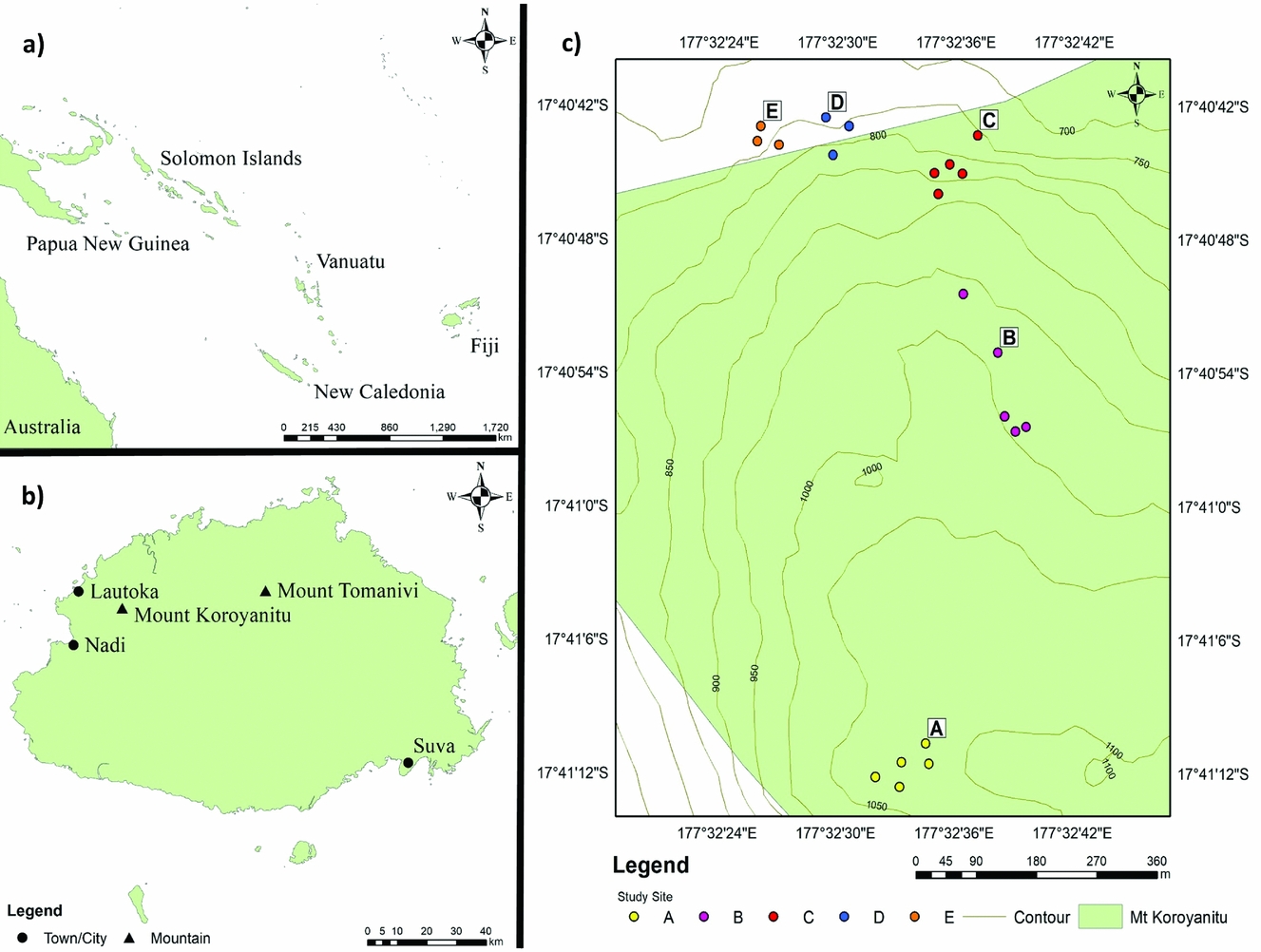
Figure 1. Location of Fiji in the South-west Pacific (a), Mount Koroyanitu on Viti Levu Island in Fiji (b), and the study plots along the western slopes of Mount Batilamu in Mount Koroyanitu National Park (c).
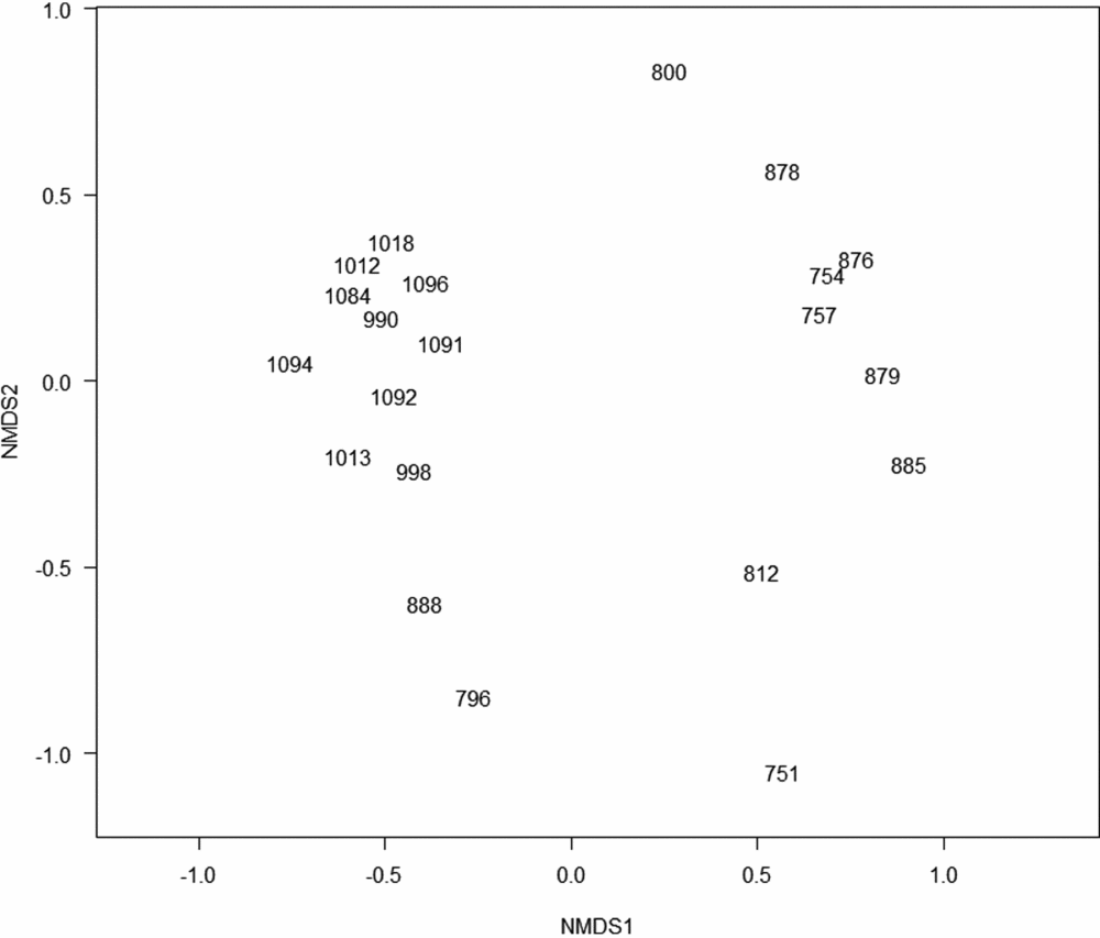
Figure 2. Non-metric MDS using the Jaccard similarity index, 21 plots along an altitudinal transect on Mount Batilamu, Viti Levu, Fiji. The plots are labelled with the altitude at which they are located.
In each plot, the following data were collected: the identity (name), dbh measured at 1.3 m above the ground, and height of each individual tree with a dbh ≥10 cm. For trees of unknown identity, herbarium-type specimens were collected, preserved in a 70% alcohol solution, pressed, transported to the South Pacific Regional Herbarium (SUVA) at the University of the South Pacific (USP), and dried at 50°C. Specimens were identified using the Flora Vitiensis Nova (Smith Reference SMITH1979–Reference SMITH1991) and herbarium collections at SUVA.
All analyses were undertaken in the R version 3.4.2 statistical computing environment (https://www.r-project.org/) using ‘ggplot’, ‘ggpubr’, ‘lme4’, ‘MASS’, ‘MuMin’ and ‘vegan’ packages. To investigate the species composition of the plots, non-metric multidimensional scaling (nMDS) was performed using the Jaccard similarity index to test for distinct forest types. A one-way Analysis of Similarity (ANOSIM; Clarke Reference CLARKE1993) using 95% (α = 0.05) confidence intervals was used to test for significant differences between forest types identified.
For each plot the following variables were measured or calculated: species richness (number of species per stem, to account for differences in stem density), endemism (proportion of species endemic to Fiji), stem density (total number of stems per plot), height (average of the five tallest trees) and volume. Tree volume was calculated assuming a conical tree shape: volume = [(dbh ÷ 2)2 × π × tree height] ÷ 3. A conical shape was assumed because it provides more conservative volume estimates than assuming a cylindrical shape, and because there were no local or regional equations for estimating volume (Magnussen & Reed Reference MAGNUSSEN and REED2015).
In addition, the relative density (number of individuals of a species ÷ total number of individuals × 100), dominance (volume of a species ÷ total volume × 100) and frequency (number of plots a species occurs in ÷ sum of frequency for all species × 100) were calculated for each species in each of two forest types. The sum of the relative density, dominance and frequency constitutes the importance value of a species (Mueller-Dombois & Ellenberg Reference MUELLER-DOMBOIS and ELLENBERG2002), which was converted to relative importance (sum of all importance values ÷ 3).
Based on visual data inspection and the small sample sizes employed, we assumed that the data collected were not normally distributed. Therefore, non-parametric tests were used; Kruskal–Wallis tests to determine significance differences between variables at the various altitudes, a Wilcoxon test to determine which altitudes or forest types differed significantly, and a Spearman rs test to identify correlations between the various variables and altitude.
Microclimate sampling and analysis
Paired Maxim iButtons (DS1923) were placed at altitudinal intervals of about 100 m, recording instantaneous readings of temperature and relative humidity every 20 min. One sensor was suspended 50 cm above the ground on bamboo sticks on the inside of inverted, white plastic cups, which were covered with white duct tape on the upper half. The other sensor was positioned inside leaf litter by placing it inside a metal tea strainer, which was covered with white duct tape on the upper (and upward-facing) half and left uncovered in the lower half (Keppel et al. Reference KEPPEL, ANDERSON, WILLIAMS, KLEINDORFER and O'CONNELL2017a). Where feasible the paired iButtons were placed in both forested and grassland vegetation at each altitude in close proximity, resulting in four iButtons per altitude; one each in the air in grasslands, leaf litter in grasslands, air in forest, and leaf litter in forest. The iButtons were mostly placed close to the plots, but we also placed a quadruplet of sensors in grassland and a forested gully at ~550 m asl.
A 48-h data window (07h00 on 19 July–06h40 on 21 July, sunshine with little cloud cover was observed during this period) was used for analyses. For this time period we calculated the average, standard deviation, maximum and minimum values of temperature and humidity for each iButton, separately for day and night time. Day and night time periods were determined by using sunrise and sunset data from timeanddate.com for the nearby city of Lautoka. The hour prior to and after sunrise and sunset were removed in order to allow a settling period between the two phases.
For both temperature and humidity, we calculated the mean, standard deviation, maximum and minimum values, separately for day- and night-time. We then used these as response variables in generalized linear mixed-effect models, with altitude as the sole fixed effect and vegetation type (open grasslands versus forest), habitat type (air versus leaf litter) and time of the day (day versus night) as random effects. We extracted the slope of the fixed effect (i.e. the lapse rate) and the percentage variance explained by each random effect from this model. We determined the significance of the fixed effect by comparing the performance of the model with and without altitude using a chi-squared test. The explanatory power of selected models was assessed using a pseudo-r 2-value (Nakagawa & Schielzeth Reference NAKAGAWA and SCHIELZETH2013), which calculates the marginal (variation explained by fixed effects) and conditional r 2 (variation explained by fixed and random effects).
RESULTS
Vegetation
Overall, there were 292 stems belonging to 71 species (in 37 families) of trees with a dbh ≥10 cm in the 21 plots. Of these, 43 species (60.56%) were endemic to Fiji. Two seemingly distinct plot clusters were produced by non-metric multidimensional scaling (nMDS; Figure 2). One group (montane plots) consisted of 10 plots at higher (>950 m) altitudes. The other group (lowland plots) consisted of plots at lower (<885 m) altitudes. The plots at 888 and 795 m had intermediate species composition, including taxa otherwise associated with higher altitudes (e.g. Podocarpus neriifolius, Podocarpaceae). The plot at 751 m was dominated by Pterocymbium oceanicum (Sterculiaceae) and was the only plot with this species. The one-way analysis of similarity (ANOSIM) supported montane and lowland plots to be significantly different (P = 0.001, r = 0.622).
The lowland plots were dominated by Dendrocnide harveyi (Urticaceae), Dysoxylum aliquantulum (Meliaceae) and Bischofia javanica (Euphorbiaceae). Together, these species accounted for more than a third of all stems and more than 60% of the total basal area, while also having the highest importance values (Table 1). The montane plots were dominated by Agathis macrophyllla (Araucariaceae), which accounted for more than 10% of all stems and almost 50% of the total tree volume. Of the 17 most important species in this study (based on being among the 10 most important species in either the lowland or montane plots), only six species occurred in both forest types (Table 1).
Table 1. Importance values of the 10 tree species with the highest importance value in either lowland or montane forest along an altitudinal transect on Mount Batilamu, Fiji. RDe = relative density (%), RDo = relative dominance (%), RF = relative frequency (%), IV = importance value (%).

Measures of species diversity (richness, endemism) and forest structure (density, height, volume) did not differ significantly among altitudes, except for volume (Kruskal–Wallis, P = 0.027). Tree volume at 1000 m asl was significantly smaller than at 750 m (P = 0.037), 900 m (P = 0.012) and 1100 m (P = 0.012). Only canopy height had a significant, linear correlation with altitude (Spearman rs, ρ = −0.9, P = 0.017). The measures of species diversity and forest structure generally displayed predicted differences between the two forest types, i.e. higher species richness and greater canopy height and tree volume in lowland forest, and higher endemism and stem density in montane forest. However, those differences were only significant for stem density (P = 0.0048).
Climate
Models consisting of altitude, vegetation type, habitat and time were good predictors of the temperature and humidity variables investigated, explaining 62–85% of the total variation (conditional r2). Altitude was a significant predictor of the average, maximum and minimum temperature, explaining about 15%, 8% and 30% of the variation in these variables, respectively (marginal r2). Time of day and vegetation type were other important predictors of these variables. Daytime temperature was generally lower in forests than in grasslands (black versus white shapes, Figure 3). The variation (standard deviation) in temperature was mostly driven by time of day (lower variation at night) and vegetation type (lower variation in forests).

Figure 3. Variation of average (19–20 July 2016) daytime temperature (a) and relative humidity (b) along an altitudinal gradient on Mount Batilamu, Fiji.
The average lapse rate was c. −0.9°C per 100 m, being higher during the day (−1.1°C per 100 m) than at night (−0.6°C per 100 m). Comparing the different microhabitats, the lapse rate was higher in grasslands (−1.15°C per 100 m in the leaf litter and −0.88°C per 100 m in the open) than in the forest (−0.86°C per 100 m in the open air and −0.64°C per 100 m in leaf litter). From about 900 m (the break between the two forest types), the average temperature did not exceed 19°C and the average relative humidity did not drop below 75%.
Altitude was a significant predictor of the average and minimum humidity (though considerably less so than for temperature), explaining about 4% and 3% of the variation in these variables, respectively (marginal r2). Habitat type, time of the day and, to a lesser extent, vegetation type were other important predictors of these variables. Daytime humidity indeed tended to be higher in leaf litter (squares) than in the air (50 cm above the ground; triangles; Figure 3). The variation (standard deviation) in humidity was mostly driven by time of day (lower variation at night), with habitat type (lower variation in leaf litter) and vegetation type (lower variation in forests) also being important. Only habitat type was a good predictor (explaining almost 60% of the total variation in this variable) of maximum humidity, with leaf litter having consistently higher maximum humidity.
DISCUSSION
The two major forest types identified along the altitudinal transect on the western slopes of Mount Batilamu correspond to lowland and montane rain forest, with the transition occurring between 800–900 m asl and corresponding with the altitude suggested for the break between these forest types (Ashton Reference ASHTON2003). The montane forest appears to be the Agathis–Podocarpus type described by Mueller-Dombois & Fosberg (Reference MUELLER-DOMBOIS and FOSBERG1998; as upland rain forest), with the conifer Agathis macrophylla as the dominant element. The montane forest is lower montane forest sensu Hamilton et al. (Reference HAMILTON, JUVIK and SCATENA1995) and Ashton (Reference ASHTON2003), as it is different from cloud forest, lacking trees with stunted growth and twisted trunks. The lowland rain forest has common lowland rain-forest elements, such as Dysoxylum spp., Bischofia javanica, Hedycarya dorstenioides and Viticipremna vitilevuensis (Keppel et al. Reference KEPPEL, TUIWAWA, NAIKATINI and ROUNDS2011). Other altitudinal transects in Fiji have similarly found turnover of dominant species with altitude (Ash Reference ASH1987, Kirkpatrick & Hassall Reference KIRKPATRICK and HASSALL1985).
Although the variables related to rain-forest diversity and structure tended to differ between lowland and montane forest as expected based on literature, the differences were more subdued than expected – with only those in stem density being significant. The limited sample size and altitudinal range of this study may have limited our ability to detect differences. Furthermore, we used the number of species endemic to Fiji (as there were no species endemic to the Mount Koroyanitu Range in our plots) and this may not respond strongly to altitude, as the percentage of endemic tree species in Fijiś lowland rain forests exceeds 50% (Keppel et al. Reference KEPPEL, BUCKLEY and POSSINGHAM2010).
Decreasing temperature and increasing relative humidity with altitude are well documented (Grubb & Whitmore Reference GRUBB and WHITMORE1966, Pepin & Losleben Reference PEPIN and LOSLEBEN2002, Shanks Reference SHANKS1954). Our lapse rates are higher than the usual average of about 0.5–0.6°C per 100 m (Osborne Reference OSBORNE2012). However, the altitudinal range that we used to calculate lapse rates was comparatively small, which can affect results (Pepin & Losleben Reference PEPIN and LOSLEBEN2002). Furthermore, lapse rates are generally calculated as the average over an entire year and our data are based on a relatively short time period during which there was little cloud cover. Lapse rates are known to differ among seasons and with cloud cover (McVicar et al. Reference MCVICAR, VAN NIEL, LI, HUTCHINSON, MU and LIU2007, Pepin Reference PEPIN2001, Pepin & Losleben Reference PEPIN and LOSLEBEN2002) and we here show that they also differ among vegetation types and in different microhabitats.
Both canopy cover and microhabitats are known to moderate microclimate (Keppel et al. Reference KEPPEL, ANDERSON, WILLIAMS, KLEINDORFER and O'CONNELL2017a, Scheffers et al. Reference SCHEFFERS, EVANS, WILLIAMS and EDWARDS2014). In our study, the absence of canopy cover strongly increased temperature and decreased relative humidity. These microclimatic differences between forests and more open vegetation, such as grasslands, savannas and canopy gaps, are well documented (Grubb & Whitmore Reference GRUBB and WHITMORE1966, Holl Reference HOLL1999, Ibanez et al. Reference IBANEZ, HELY and GAUCHEREL2013, Turton & Sexton Reference TURTON and SEXTON1996). The leaf-litter microhabitat strongly moderated climatic variables, especially relative humidity. In addition, topographic variation can strongly affect microclimate measurements (Lookingbill & Urban Reference LOOKINGBILL and URBAN2003). While we minimized the effects of aspect, which can be significant, we could not include other important effects, such as solar radiation and distance to a stream (Lookingbill & Urban Reference LOOKINGBILL and URBAN2003), as fine-scale digital elevation models (DEMs) are not available for the area.
Only recently has the ability of microhabitats to retain microclimates that are more stable than external conditions been quantified and its potential importance under anthropogenic climate change been realized (Keppel et al. Reference KEPPEL, ANDERSON, WILLIAMS, KLEINDORFER and O'CONNELL2017a, Scheffers et al. Reference SCHEFFERS, EVANS, WILLIAMS and EDWARDS2014). As such microhabitats can maintain more consistent and favourable climates and, therefore, they are likely to be important in facilitating the persistence of biota as regional environmental conditions change (Lenoir et al. Reference LENOIR, HATTAB and PIERRE2017, Scheffers et al. Reference SCHEFFERS, EVANS, WILLIAMS and EDWARDS2014). Our study shows that vegetation and microhabitats interact to create a patchwork of microclimates (Keppel et al. Reference KEPPEL, ANDERSON, WILLIAMS, KLEINDORFER and O'CONNELL2017a), which is important for facilitating the persistence of species under forecast anthropogenic climate change, as species respond to this fine-scale interplay of abiotic and biotic factors (Keppel et al. Reference KEPPEL, ROBINSON, WARDELL-JOHNSON, YATES, VAN NIEL, BYRNE and SCHUT2017b, Oorebeek & Kleindorfer Reference OOREBEEK and KLEINDORFER2008).
Our findings therefore highlight the importance of including the moderating effects of vegetation and microhabitats on climatic conditions when forecasting future changes in climate and species distributions. This even holds true for the tropical South-West Pacific islands, which are experiencing milder climate change than higher latitudes (IPCC 2014). However, climatic data are currently mostly derived from meteorological stations in open areas without tall vegetation and we therefore cannot currently quantify the effects of canopy cover on microclimate (De Frenne & Verheyen Reference DE FRENNE and VERHEYEN2016).
ACKNOWLEDGEMENTS
We would like to thank Abaca Village, Vuda District, Ba Province, for kindly giving us permission for, and providing assistance, during the fieldwork. Geon C. Hanson and Leomar Longsworth assisted with data collection. This research was undertaken as part of a joint undergraduate student project between Flinders University, the University of South Australia and the University of the South Pacific, and funded through the Department of Foreign Affairs and Trade of the Australian Government as part of the New Colombo Plan initiative. During part of the analyses and writing GK was supported by an Alexander von Humboldt fellowship. A study tour travel grant by the University of South Australia assisted JA, SMT, AR and TC.


