


1 Introduction
Convective turbulent flows are ubiquitous in nature and play a central role in, for example, geophysical systems including atmospheric and oceanic dynamics as well as those in the mantle and core of the Earth (McKenzie, Roberts & Weiss Reference McKenzie, Roberts and Weiss1974; Hartmann, Moy & Fu Reference Hartmann, Moy and Fu2001). Rayleigh–Bénard (RB) convection is a fundamental phenomenon that has become a paradigm for thermal-driven flows in which a fluid layer is heated at the bottom and cooled at the top. Understanding of RB turbulence is instrumental to uncover complex convection phenomena occurring in nature and engineering processes (Zhou, Sun & Xia Reference Zhou, Sun and Xia2007; Lohse & Xia Reference Lohse and Xia2010). In many scenarios convective flows contain suspended particles such as water droplets in clouds, bubbles and plankton distributions in the oceans and pollutants in the atmospheric boundary layer (Toschi & Bodenschatz Reference Toschi and Bodenschatz2009; Bourgoin & Xu Reference Bourgoin and Xu2014). In particular, buoyant particles and their dynamics including path instability can enhance mixing and heat transfer in industrial reaction catalysis (Magnaudet & Eames Reference Magnaudet and Eames2000; Lakkaraju et al. Reference Lakkaraju, Stevens, Oresta, Verzicco, Lohse and Prosperetti2013).
Experimental investigations of Lagrangian dynamics in convective turbulence have primarily focused on the flow using tracer particles (Ni, Huang & Xia Reference Ni, Huang and Xia2012; Ni & Xia Reference Ni and Xia2013; Liot et al. Reference Liot, Gay, Salort, Bourgoin and Chillà2016; Kim et al. Reference Kim, Shen, Dimarco, Jin and Chamorro2018), whereas the majority of studies on the Lagrangian dynamics of particle-laden flows have explored the acceleration statistics in homogeneous isotropic turbulence (La Porta et al. Reference La Porta, Voth, Crawford, Alexander and Bodenschatz2001; Bourgoin et al. Reference Bourgoin, Ouellette, Xu, Berg and Bodenschatz2006; Mathai et al. Reference Mathai, Huisman, Sun, Lohse and Bourgoin2018a). Pair dispersion in turbulence is defined as  $R^{2}(t)=\langle [r_{p}(t)-r]^{2}\rangle$, where
  $r_{p}(t)$ is the distance between two trajectories as a function of time and
  $r$ is the initial separation. Very recently, Mathai et al. (Reference Mathai, Huisman, Sun, Lohse and Bourgoin2018a) investigated dispersion of air bubbles in isotropic turbulence at Taylor-scale Reynolds numbers ranging from 110 to 310. They found two regimes in the bubble dispersion characterized by ballistic growth (
 $\propto t^{2}$) at short times, which approached a diffusive regime (
 $\propto t^{1}$) at sufficiently large times; we note that Mathai et al. (Reference Mathai, Huisman, Sun, Lohse and Bourgoin2018a) did not explore the effect of initial separation.
Batchelor (Reference Batchelor1950) first predicted that the initial separation  $r$ between a pair of fluid particles in isotropic homogeneous turbulence is an important parameter in
  $R^{2}(t)$. Below a characteristic time,
  $t_{0}=(r^{2}/\unicode[STIX]{x1D716})^{1/3}$, where
  $\unicode[STIX]{x1D716}$ is the mean kinetic energy dissipation rate, the pair dispersion exhibits a relation
  $R^{2}(t)=f(r)t^{2}$. The function
  $f(r)$ can be obtained from the second-order longitudinal and transverse Eulerian structure functions (Bourgoin et al. Reference Bourgoin, Ouellette, Xu, Berg and Bodenschatz2006; Ni & Xia Reference Ni and Xia2013). Many flows contain millimetric-sized bubbles with diameters
  $d_{b}$ in the range of 1–2 mm. In such cases, buoyancy results in relatively large bubble rise velocities
  $u_{b}\approx \sqrt{gd_{b}}$, which leads to large Weber
  $We=\unicode[STIX]{x1D70C}_{f}u_{b}^{2}d_{b}/\unicode[STIX]{x1D70E}$ and Reynolds
  $Re=u_{b}d_{b}/\unicode[STIX]{x1D708}$ numbers (Clift, Grace & Weber Reference Clift, Grace and Weber1978; Mathai et al. Reference Mathai, Huisman, Sun, Lohse and Bourgoin2018a). Here,
  $g$ is the gravity,
  $\unicode[STIX]{x1D70C}_{f}$ is the fluid density,
  $\unicode[STIX]{x1D70E}$ is the surface tension and
  $\unicode[STIX]{x1D708}$ is the kinematic viscosity of the fluid. Also recently, Mathai et al. (Reference Mathai, Zhu, Sun and Lohse2018b) characterized the path and wake instability mechanisms of buoyant particles in turbulent flows by modulating the particle’s moment of inertia. As a result, the particle may exhibit path instability and wake-induced motions, resulting in rich interactions between bubbles and flow (Mougin & Magnaudet Reference Mougin and Magnaudet2001; Bunner & Tryggvason Reference Bunner and Tryggvason2003; Roghair et al. Reference Roghair, Mercado, Annaland, Kuipers, Sun and Lohse2011; Ern et al. Reference Ern, Risso, Fabre and Magnaudet2012; Mathai et al. Reference Mathai, Prakash, Brons, Sun and Lohse2015; Alméras et al. Reference Alméras, Mathai, Lohse and Sun2017; Mathai et al. Reference Mathai, Zhu, Sun and Lohse2018b). In relatively weak and strongly anisotropic turbulence of RB convection, the path instability of buoyant particles and the initial separation of bubble pairs may play an important role in the particle-flow dynamics.
Our understanding of the interaction between inertial particles and convective turbulence, in particular the effect of initial separation, is limited. In this work we explore the pair dispersion of millimeter-size bubbles in RB convection over a wide range of initial separations. The involved phenomena are complex and offer multiple experimental challenges. Our setup considered uniform bubble release with a flux that did not produce accumulation at the top plate to avoid local changes in the heat transfer. A sufficiently large interrogation volume was used to track bubbles at large initial separations.
2 Approach
2.1 Experimental setup

Figure 1. (a) Schematic of the experimental setup. (b) Basic diagram illustrating the diagonal coordinate system,  $s$, with origin at the centre of the bottom wall, and aligned with the convective roll. The locations of the bubble generator were
  $s/D=-1/2,0$ and
  $1/2$.
Experiments were carried out in a  $500~\text{mm}\times 500~\text{mm}$ cross-section RB tank (Kim et al. Reference Kim, Shen, Dimarco, Jin and Chamorro2018) with a height
  $H=400~\text{mm}$, i.e. aspect ratio of
  $\unicode[STIX]{x1D6E4}=\text{side}/\text{height}=1.25$, which was filled with deionized water (figure 1a). The vertical walls of the tank are made of double-pane insulated/evacuated tempered glass panels. Each pane is 3.175 mm thick and separated by a 9.525 mm barrier of inert gas. The glass walls were adhered to each other (and sealed) using high-temperature water-resistant RTV silicone. The base (heater portion) of the tank consists of an 800 W,
  $457.2~\text{mm}\times 457.2~\text{mm}$ flat silicone heater adhered to the underside of a 11 mm thick aluminum plate (using high temperature silicone adhesive). The back side of the heating element is lined with a high-temperature pyramidal patterned silicone matte layer, which provides an encapsulated air barrier for primary insulation. A 63.5 mm thick layer of fire foam was applied over the matte layer, and encased within a wooden frame. As a precaution, the closest surfaces of the wooden frame are (a minimum of) 25 mm from the edge of the silicone heating element to ensure that the wooden frame remains at regular conditions. A temperature sensing bulb was set in contact with the underside of the heating element and embedded within the foam, and was kept from direct contact with the foam and the wood with a 25 mm air gap within an aluminum sheet-metal heat shield. The frame is capped off with a 9.5 mm aluminum plate that serves as the seating surface of the underside of the tank. The edges of the inside surface of the base plate are adhered (and sealed) to the glass walls with high-temperature water-resistant RTV silicone. The surface of the base plate (exposed to water) is coated with seven layers of high-temperature water-resistant flat-black ceramic paint. The entire tank is finished in a solid oak trim, which is secured with fibreglass mesh impregnated with high-temperature silicone adhesive. A cooling plate hangs from the top of the tank with adjustable hanging height, connected to a 1000 W capacity PolyScience (Model AD15R-30-A11B) refrigerated circulator. Insulating foam panels are attached to the top of the cooling plate and the side walls.
Three high-speed CMOS ( $2048~\text{pixels}\times 2048~\text{pixels}$) cameras were mounted perpendicularly to capture the rising bubbles. Four LED light bars were installed at the tank corners and used to illuminate the bubbles. Each camera had an investigation area of
  $250~\text{mm}\times 400~\text{mm}$, leading to a total investigation volume of
  $250~\text{mm}\times 250~\text{mm}\times 400~\text{mm}$. It covered
  $s/D\in [-0.5,0.5]$ and
  $z/H\in [0,1]$, where
  $s$ is the distance along a diagonal from the origin set at the centre of the bottom of the tank,
  $z$ is the vertical coordinate,
  $H=400~\text{mm}$, and
  $D=283~\text{mm}$ is half of the diagonal length of the RB tank (figure 1b). For each case, 1800 consecutive sets of three-view images were captured with the three, 4 MP cameras at 200 Hz. Seven distinct setups were measured, where one of them with a quiescent medium served as a base case. Before each measurement, the flow was run for at least 30 min to allow stable RB convection before using the bubble generators. The bubbles were tracked 10 s after the release to exclude potential transient effects. Bubbles on the top plate were removed prior to every test to minimize local effects on the top wall.
Convective flows were induced with two temperature differences,  $\unicode[STIX]{x0394}T=5\,^{\circ }\text{C}$ and
  $10\,^{\circ }\text{C}$, resulting in Rayleigh numbers of
  $Ra=g\unicode[STIX]{x1D6FC}\unicode[STIX]{x0394}TH^{3}/\unicode[STIX]{x1D705}\unicode[STIX]{x1D708}\approx 5.5\times 10^{9}$ and
  $1.1\times 10^{10}$, Nusselt numbers of
  $Nu=QH/\unicode[STIX]{x1D706}\unicode[STIX]{x0394}T\approx 200$ and 400, and Prandtl numbers of
  $Pr=\unicode[STIX]{x1D708}/\unicode[STIX]{x1D705}\approx 5.4$. Both cases exhibited similar results; consequently, we show the
  $Ra=1.1\times 10^{10}$ case for brevity, unless pointed out explicitly. The local Kolmogorov length scale was
  $\unicode[STIX]{x1D702}=(\unicode[STIX]{x1D708}^{3}/\langle \unicode[STIX]{x1D716}\rangle )^{1/4}\approx 8\times 10^{-4}~\text{m}$. Here,
  $g$ is the gravitational acceleration,
  $\unicode[STIX]{x1D6FC}$ is the thermal expansion coefficient,
  $\unicode[STIX]{x1D705}$ is the thermal diffusivity,
  $Q$ is the heat flux across the cell and
  $\unicode[STIX]{x1D706}$ is the thermal conductivity of the fluid. The bulk dissipation rate was estimated as
  $\langle \unicode[STIX]{x1D716}\rangle =RaPr^{-2}(Nu-1)\unicode[STIX]{x1D708}^{3}/H^{4}\approx 1.6\times 10^{-6}~\text{m}^{2}~\text{s}^{-3}$ (Kim et al. Reference Kim, Shen, Dimarco, Jin and Chamorro2018). The Reynolds number of the convection system corresponding to the turnover time of thermal excitation was estimated as
  $Re_{c}=0.138Pr^{-0.82}Ra^{0.493}\approx 3\times 10^{3}$ (Brown, Funfschilling & Ahlers Reference Brown, Funfschilling and Ahlers2007). A measurement sampling rate of 200 Hz allowed for inspection of the trajectories at sub-Kolmogorov time scales given by
  $\unicode[STIX]{x1D70F}=\sqrt{\unicode[STIX]{x1D708}/\langle \unicode[STIX]{x1D716}\rangle }\approx 0.8~\text{s}$. The total measurement time was
  $11.25\unicode[STIX]{x1D70F}$ (i.e.,
  ${\approx}10~\text{s}$), which is considered sufficient to track full bubble trajectories in the system as bubbles reach the top plate approximately
  $4~\text{s}$ after release. Measurements were repeated twice after reaching stable RB convection. Additional details of the convection tank and parameters of the RB convection can be found in Kim et al. (Reference Kim, Shen, Dimarco, Jin and Chamorro2018). Two air bubble streams were generated from two porous stones connected to a 4 W air pump. The size of the bubbles were
  $d_{b}=0.96\pm 0.15~\text{mm}$, or
  $1.2\pm 0.2\unicode[STIX]{x1D702}$, with a bulk rising velocity in a quiescent medium of
  $u_{b}\approx 0.09~\text{m}~\text{s}^{-1}$. The bubble volume fraction,
  $\unicode[STIX]{x1D719}_{v}\approx 1\times 10^{-6}$, and the surface fraction of the bubble’s accumulation on the top plate,
  $\unicode[STIX]{x1D719}_{s}\approx 5\times 10^{-4},$ during each measurement resulted in negligible effects on the overall flow (Elghobashi Reference Elghobashi1994). The bubble generator was placed in one of the diagonal axes along the roll structure at
  $s/D=-1/2$,
  $-1/4$, 0,
  $1/4$ and
  $1/2$, where
  $s$ is the distance along the diagonal with respect to the centre of the tank. The positive and negative values of
  $r$ indicate bubble release within the upward and downward motions of the convective roll. Bubbles were released individually at a rate of 10.7 bubbles
  $\text{s}^{-1}$ from the single source hole of the bubble generator. This formed a single column of rising bubbles in the vicinity of the source.
The air bubbles were tracked using a three-dimensional (3-D) particle tracking velocimetry (3-D PTV). The 3-D calibration was performed using a planer target at multiple planes. The resulting root mean square of the recognized calibration points was of the order of  $10^{-2}\unicode[STIX]{x1D702}$. For each case, approximately
  $5\times 10^{3}$ trajectories with an average of 122 frames and a total of
  $5.5\times 10^{5}$ data samples were tracked using the Hungarian algorithm (Luetteke, Zhang & Franke Reference Luetteke, Zhang and Franke2012), and linked by performing a three-frame gap closing for reconstructing longer trajectories. Approximately 300 bubbles were tracked simultaneously, allowing for the characterization of various initial separations. Bubble trajectories and associated temporal derivatives were filtered and estimated using fourth-order
  $B$ splines (Craven & Wahba Reference Craven and Wahba1978). Additional details of the PTV setup can be found in Kim et al. (Reference Kim, Kim, Liberzon and Chamorro2016a,Reference Kim, Zhang, Liberzon, Zhang and Chamorrob, Reference Kim, Shen, Dimarco, Jin and Chamorro2018).
2.2 Numerical simulations
Complementary numerical simulations under the same conditions as the experiments were carried out to assess the effect of path instability. Direct numerical simulations were carried out to simulate the fully developed convection in the RB tank. The governing equations for the incompressible fluid flow under the Boussinesq approximation are given by
 $$\begin{eqnarray}\displaystyle & \displaystyle \frac{\unicode[STIX]{x2202}\boldsymbol{u}}{\unicode[STIX]{x2202}t}+(\boldsymbol{u}\boldsymbol{\cdot }\unicode[STIX]{x1D735})\boldsymbol{u}=-\frac{1}{\unicode[STIX]{x1D70C}}\unicode[STIX]{x1D735}p+\unicode[STIX]{x1D708}\unicode[STIX]{x1D6FB}^{2}\boldsymbol{u}-\boldsymbol{g}\unicode[STIX]{x1D6FD}T, & \displaystyle\end{eqnarray}$$
 $$\begin{eqnarray}\displaystyle & \displaystyle \unicode[STIX]{x1D735}\boldsymbol{\cdot }\boldsymbol{u}=0, & \displaystyle\end{eqnarray}$$
 $$\begin{eqnarray}\displaystyle & \displaystyle \frac{\unicode[STIX]{x2202}T}{\unicode[STIX]{x2202}t}+(\boldsymbol{u}\boldsymbol{\cdot }\unicode[STIX]{x1D735})T=\unicode[STIX]{x1D705}\unicode[STIX]{x1D6FB}^{2}T, & \displaystyle\end{eqnarray}$$
 where  $\boldsymbol{u}$,
  $p$ and
  $T$ are the fluid velocity, pressure and temperature, respectively, and
  $\unicode[STIX]{x1D70C}$,
  $\unicode[STIX]{x1D708}$,
  $\unicode[STIX]{x1D6FD}$, and
  $\unicode[STIX]{x1D705}$ are the density, kinematic viscosity, thermal expansion coefficient and thermal diffusivity of the fluid, respectively. The governing equations were discretized in space by a second-order finite difference method, and a hybrid third-order Runge–Kutta method was used for the temporal advancement. The Poisson equation for the pressure is directly solved by using a discrete cosine transform. A no-slip boundary condition is applied at all walls. The temperature was maintained constant at the top and bottom surfaces, and an adiabatic condition was applied to the side walls. We considered 256 uniform grids distributed in each horizontal direction, and 128 non-uniform grids in the vertical direction to accurately capture the steep temperature gradient near the top and bottom surfaces. In addition, we carried out two extra simulations with resolutions of
  $256\times 256\times 256$ (vertically doubled grids) and
  $384\times 384\times 128$ (horizontally doubled grids). The flow field and temperature were hardly affected by the increase in the resolution. In addition, the difference in the Nusselt numbers for all three cases was found to be within 1.5 %. See additional details in the Appendix.
Bubble motion was simulated by the point-bubble approximation based on the Stokes flow (Mazzitelli & Lohse Reference Mazzitelli and Lohse2003; Fouxon et al. Reference Fouxon, Shim, Lee and Lee2018):
 $$\begin{eqnarray}\displaystyle & \displaystyle \frac{\text{d}\boldsymbol{x}}{\text{d}t}=\boldsymbol{v}, & \displaystyle\end{eqnarray}$$
 $$\begin{eqnarray}\displaystyle & \displaystyle \frac{\text{d}\boldsymbol{v}}{\text{d}t}=-\frac{\boldsymbol{v}-\boldsymbol{u}}{\unicode[STIX]{x1D70F}_{b}}-2\boldsymbol{g}+3\frac{\text{D}\boldsymbol{u}}{\text{D}t}+\unicode[STIX]{x1D74E}\times (\boldsymbol{v}-\boldsymbol{u}). & \displaystyle\end{eqnarray}$$
 Here  $\boldsymbol{x}$ and
  $\boldsymbol{v}$ are the position and velocity of a bubble,
  $\boldsymbol{u}$ is the fluid velocity at the bubble’s position,
  $\unicode[STIX]{x1D74E}$ is the fluid vorticity at the bubble’s position and
  $\unicode[STIX]{x1D70F}_{b}=d_{b}^{2}/(24\unicode[STIX]{x1D708})$ is the bubble’s time scale. For the calculation of
  $\boldsymbol{u}$ and
  $\unicode[STIX]{x1D74E}$, the fourth-order Hermite interpolation (Choi, Yeo & Lee Reference Choi, Yeo and Lee2004; Lee, Yeo & Choi Reference Lee, Yeo and Choi2004) was used and the third-order Runge–Kutta scheme was adopted in the temporal advancement of (2.4) and (2.5). We assumed a one-way coupling between the fluid and bubbles in the computations.
3 Results

Figure 2. Sample of 3-D trajectories of rising bubbles in (a) quiescent medium and (b) convective turbulence at  $s/D=1/2$; the colour bar denotes the bubbles, lateral velocity,
  $u_{L}$, normalized by the local Kolmogorov length scale,
  $\unicode[STIX]{x1D70F}/\unicode[STIX]{x1D702}$. Dimensionless vertical profiles of (a) the lateral velocity component
  $u_{L}$ and (b) the standard deviations
  $\unicode[STIX]{x1D70E}_{u}$ at
  $s/D=1/4$ (▫) and
  $1/2$ (experiment,
  $\times$, and DNS,
  $\ast$, for
  $Ra=1.1\times 10^{10}$). The case with quiescent medium (○) is also included for reference.
Unlike isotropic homogeneous turbulence, the convective turbulence is highly anisotropic. Dynamics of the bubbles is likely to exhibit distinct behavior; in particular, the effect of initial separation may indicate different modulating processes depending on the location. Approximately 1200 sample 3-D trajectories of rising bubbles tracked for approximately 90 frames by 3-D PTV for both a quiescent flow and convective turbulence are shown in figure 2(a,b). It shows a notorious curved path of the bubbles induced by the roll structure; note also the reduced lateral diffusion with respect to the quiescent case. Enhanced path instability dynamics may modulate such a feature in the latter. The distinct dynamics of the bubbles in the RB convection is first assessed from the mean and standard deviation of the vertical profiles of the lateral velocity component,  $u_{L}$. The profiles at
  $s/D=1/4$ and
  $1/2$ for the
  $Ra=1.1\times 10^{10}$ cases are illustrated in figure 2(c,d), we also include the case with a quiescent medium for reference. It is worth pointing out that similar trends were observed in the other
  $Ra$ case, which is not shown for brevity. Note the
  $u_{L}\approx 0$ near the bottom wall under the quiescent medium, and the footprint of the path instability due to the inertial behavior of the bubbles at later stages of the rising process. In the case of the bubble rising under convection,
  $u_{L}$ revealed a sustained influence of the flow with a
  $u_{L}\approx 0$ at the tank half height,
  $h=H/2$, independent of
  $s/D$. This evidenced the effect of a convective roll structure on the inertial particles and a bulk dynamical symmetry. Notably, the standard deviation of the bubbles lateral velocity,
  $\unicode[STIX]{x1D70E}_{u}$, significantly decreased with the presence of convection; it was also roughly constant along the vertical path. This indicates that the convective turbulence constrained the path instability of the bubbles. Numerical prediction of the mean lateral velocity of the bubbles shows good agreement with the measured data, whereas the standard deviation is underestimated. This indicates that the convective motion tends to suppress the path instability of the bubbles, but not completely, given that the numerical model of bubble motion ((2.4) and (2.5)) is incapable of simulating the path instability.

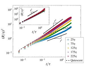
Figure 3. Dimensionless pair dispersion  $R^{2}/\unicode[STIX]{x1D702}^{2}$ in the quiescent medium for (a) the vertical and (b) the lateral directions as a function of dimensionless time
  $t/\unicode[STIX]{x1D70F}$ for various initial separations,
  $r$, ranging from
  $25\unicode[STIX]{x1D702}$ to
  $225\unicode[STIX]{x1D702}$. The inset illustrates the compensated pair dispersion by
  $t^{1}$ (
 $\times$) and
  $t^{2}$ (○).
As discussed by Bourgoin et al. (Reference Bourgoin, Ouellette, Xu, Berg and Bodenschatz2006), the pair dispersion of tracers in a quiescent medium undergo Brownian motion with a linear relation  $R^{2}\propto t^{1}$. However, this is not the case for these buoyant particles in the quiescent medium. Pair dispersion,
  $R^{2}(t)$, of rising bubbles in the quiescent flow were obtained for various initial separations,
  $r$; see figure 3(a,b). Over 5000 data points were averaged at each instant and initial separation with a tolerance of
  $r\pm 25\unicode[STIX]{x1D702}$ for all cases. The vertical component of
  $R^{2}(t)$ exhibited a trend proportional to
  $t^{2}$ throughout the temporal span of
  $0.007<t/\unicode[STIX]{x1D70F}<2$, indicating the buoyancy effect of rising bubbles following the Batchelor scaling (figure 3a). The lateral component of
  $R^{2}(t)$ shown in figure 3(b), where the effect of path oscillation is dominant, underwent a ballistic to diffusive transition (
 $t^{2}$-to-
 $t^{1}$). The transition occurred at
  $t=t_{St}\approx 0.14$ s which is the intrinsic property of the bubble. This ballistic-to-diffusive transition observed in the quiescent medium showed similarities with a previous study by Mathai et al. (Reference Mathai, Huisman, Sun, Lohse and Bourgoin2018a) on the dispersion of bubbles in isotropic turbulence. In their work,
  $R^{2}$ grew ballistically following a
  $t^{2}$-trend within short times, and approached a diffusive
  $t^{1}$-regime at larger times. Although these phenomena were observed in isotropic turbulence, they concluded that the early ballistic-to-diffusive transition compared to the flow was due to the intrinsic characteristics of rising bubbles including unsteady wake-induced motions and path instability. It is worth noting that the ballistic regime is relatively short in the quiescent medium as shown in the compensated pair dispersion (inset of figure 3b).

Figure 4. Dimensionless lateral pair dispersion  $R^{2}/\unicode[STIX]{x1D702}^{2}$ in the
  $Ra=1.1\times 10^{10}$ scenario at (a)
  $s/D=1/2$ and (b)
  $s/D=0$ as a function of dimensionless time
  $t/\unicode[STIX]{x1D70F}$ for various initial separations (
 $25\unicode[STIX]{x1D702}$ to
  $225\unicode[STIX]{x1D702}$). The dashed line indicates the case in a quiescent flow. The insets in plots (a) and (b) show the vertical pair dispersion at
  $s/D=1/2$ and the bulk pair dispersion at
  $s/D=0$ (blue) and
  $s/D=0.5$ (red), respectively.
The bulk pair dispersion, equivalent to  $R^{2}$ averaged over the entire range of measured initial separations
  $0<r<250$, and within
  $s/D=0$ and
  $1/2$ is shown in the inset of figure 4(b). As the turbulence and anisotropy increased with increasing
  $s/D$ (see the Appendix), the dispersion rate increased, deviating from the diffusive regime. The bulk pair dispersion exhibited a combined
  $t^{1.5}$-relation, which is in between the ballistic and diffusive regimes. To uncover details of this phenomenon,
  $R^{2}$ is quantified for various initial separations,
  $r$, in the vertical and lateral directions at
  $s/D=1/2$. The
  $R^{2}$ in the vertical direction (figure 4a inset) did not change with
  $r$, and exhibited a similar trend as the quiescent case (figure 3a). This indicates that
  $R^{2}$ in the vertical direction is dominated by the buoyancy, and not affected by the convective turbulence due to its relatively weak magnitude in that direction. The collapsed dispersion trend in the vertical direction further indicates that the size effect of the roll structure constrained by the convection tank did not affect the dispersion within the temporal span of
  $0.007<t/\unicode[STIX]{x1D70F}<2$. However,
  $R^{2}$ exhibited a clear trend with respect to the initial separation in the lateral direction (figure 4a). Particle pairs dispersed relatively slow at short times and initial separations with
  $R^{2}\propto t^{1}$. This was followed by
  $R^{2}\propto t^{2}$ at sufficiently large times and initial separations, exceeding the dispersion under quiescent flow. The range of trends of
  $R^{2}$ between
  $t^{1}$ and
  $t^{2}$ with respect to the initial separation resulted in the bulk
  $t^{1.5}$ behavior. At
  $s/D=0$,
  $R^{2}$ underwent a transition phase similar to the ballistic-to-diffusive regime in the vicinity of the cell centre, and the effect of
  $r$ is less predominant than the case when
  $s/D=1/2$ (figure 4b).

Figure 5. Pair dispersion difference with a grid resolution of  $200\times 560$, ranging from
  $r/\unicode[STIX]{x1D702}=25\pm 25$ to
  $275\pm 25$ with
  $\unicode[STIX]{x0394}r/\unicode[STIX]{x1D702}=1.25$ and from
  $t/\unicode[STIX]{x1D70F}=0$ to 3.5 with
  $\unicode[STIX]{x0394}t/\unicode[STIX]{x1D70F}=0.0063$,
  $(R^{2}-R_{0}^{2})/\unicode[STIX]{x1D702}^{2}$, between convective and quiescent cases at (a)
  $s/D=0.5$ and (b)
  $s/D=-0.5$ for
  $Ra=1.1\times 10^{10}$. The dashed lines denote
  $(R^{2}-R_{0}^{2})/\unicode[STIX]{x1D702}^{2}\approx 0$.
The difference in pair dispersion between the convective and quiescent cases,  $(R^{2}-R_{0}^{2})/\unicode[STIX]{x1D702}^{2}$, as a function of time and initial separation is obtained to quantify the effect of the convective turbulence on the intrinsic characteristics of the dynamics of the bubbles (figure 5a,b). As the time
  $t/\unicode[STIX]{x1D70F}$ and initial separation
  $r/\unicode[STIX]{x1D702}$ increased, the difference
  $(R^{2}-R_{0}^{2})/\unicode[STIX]{x1D702}^{2}$ increased. This indicates that the convective turbulence enhanced the pair dispersion at large times as well as initial separations, and modified the intrinsic dynamics of the bubbles. The critical time
  $t_{c}$ as a function of initial separation
  $r$, where
  $(R^{2}-R_{0}^{2})/\unicode[STIX]{x1D702}^{2}\approx 0$, shows that when
  $t_{c}>t_{St}$,
  $t_{c}$ decreased with
  $r^{-3/2}$, and when
  $t<t_{St}$,
  $t_{c}$ decreases at a higher rate (figure 6a). The results indicate that the pair dispersion of the rising bubbles induced by convective turbulence exceeded the quiescent case faster as the initial separation increased. In addition, the rate of this critical time decreased faster during
  $t_{c}<t_{St}$ compared to that when
  $t_{c}>t_{St}$, where the effect of convective turbulence dominated and enhanced dispersion. The sum of the difference
  $M=\sum _{r=0}^{r=250\unicode[STIX]{x1D702}}\sum _{t=0}^{t=2\unicode[STIX]{x1D70F}}(R^{2}-R_{0}^{2})/\unicode[STIX]{x1D702}^{2}$ as a function of
  $s/D$ is computed to quantify the total difference between the pair dispersion in the quiescent and convective cases for various initial separations (see inset of figure 6a). The sum of the difference
  $M$ increased as the turbulence intensity and anisotropy increased. This indicates that higher turbulence intensity and anisotropy enhance pair dispersion, deviating from the case of the quiescent condition.

Figure 6. (a) Critical pair dispersion  $t_{c}/\unicode[STIX]{x1D70F}$, where
  $(R^{2}-R_{0}^{2})/\unicode[STIX]{x1D702}^{2}=0$, as a function of initial separation
  $r/\unicode[STIX]{x1D702}$ and time
  $t/\unicode[STIX]{x1D70F}$. The inset shows the sum
  $M=\sum _{r=0}^{r=250\unicode[STIX]{x1D702}}\sum _{t=0}^{t=2\unicode[STIX]{x1D70F}}(R^{2}-R_{0}^{2})/\unicode[STIX]{x1D702}^{2}$ at various
  $s/D$. (b) Lagrangian time correlation
  $C_{uu}$ of the lateral velocity of the bubbles as a function of time normalized by the bubble vortex-shedding time scale
  $t_{St}=1/f_{0}$.
To add insight into the effect of convective turbulence on path instability of the bubbles, the autocorrelation function (ACF) of the horizontal velocity of the bubble is illustrated in figure 6(b). This quantity exhibits oscillations at a frequency of  $f_{0}\approx 7.0~\text{Hz}$ and a Strouhal number
  $St=(f_{0}d_{b}/u_{b})\approx 0.07$, where
  $u_{b}/d_{b}\approx 100$, similar to previous works (Mougin & Magnaudet Reference Mougin and Magnaudet2001; Mathai et al. Reference Mathai, Huisman, Sun, Lohse and Bourgoin2018a). Mathai et al. (Reference Mathai, Huisman, Sun, Lohse and Bourgoin2018a) recently found that
  $f_{0}$ does not have clear dependency on turbulence in homogeneous and isotropic turbulence. Here, we show that the roll structures of the convective cell did not affect the oscillation frequency. Despite the fact that
  $f_{0}$ and
  $St$ were not affected by the convective turbulence, the ACF amplitude of the oscillations decreased with increased distance from the cell centre, indicating that the convective turbulence reduced the bubbles wake-induced motions.
4 Conclusions
In summary, we have explored the dynamics of rising air bubbles in Rayleigh–Bénard convection both experimentally and numerically for the first time. In addition to the effect of inhomogeneity and anisotropy induced by the natural convection on the dispersion of buoyant particles, we explored the pair dispersion in a wide range of initial separations by tracking a large number of bubbles at various locations of the convection cell. Near the centre of the convective cell, where the flow exhibits features of homogeneity and isotropy, the pair dispersion of air bubbles underwent a transition similar to the ballistic-to-diffusive ( $t^{2}$-to-
 $t^{1}$) regime, comparable to the case of isotropic turbulence (Mathai et al. Reference Mathai, Huisman, Sun, Lohse and Bourgoin2018a). Away from the cell centre, where the inhomogeneity and anisotropy increased, the pair dispersion increased to
  $t^{3/2}$ in the diffusive regime.
  $R^{2}$ exhibited a
  $t^{1}$ trend at small initial separations and a
  $t^{2}$ trend at large initial separations, resulting in a
  $t^{3/2}$ bulk dispersion behavior. At small
  $r$, the convective turbulence reduced the fluctuations of the bubbles, which are due to their intrinsic characteristics of the rising motion, namely, unsteady wake-induced and path instability effects. At large
  $r$, the inhomogeneous and anisotropic nature of the roll structure enhanced the pair dispersion. The findings further reveal that the path instability of bubbles plays a major role in the pair dispersion even in the presence of convection motion. Our study shows the importance of initial separation in the dispersion dynamics of air bubbles, which provides a better understanding towards the mixing mechanisms in convective bubbly flows with applications in oceanic flows and industrial processes (Magnaudet & Eames Reference Magnaudet and Eames2000). Future work will inspect the bubble dynamics of various sizes as well as aspect ratios of the convection tank, and characterization of the flow field around the buoyant particles to uncover the interaction between the bubbles’ wake and convective turbulence.
Acknowledgements
This research was funded by the National Science Foundation, grant no. CBET-1912824. The work by C.L. was supported by Samsung Science and Technology Foundation (SSTF- BA1702_03).
Declaration of interests
The authors report no conflict of interest.
Appendix. On the validation of the simulations
Here we validated our numerical simulation against the 3-D RB convection experiment by Vasiliev et al. (Reference Vasiliev, Sukhanovskii, Frick, Budnikov, Fomichev, Bolshukhin and Romanov2016), which was conducted in almost the same experimental setting as our experiments. The side length is 250 mm and the aspect ratio is 1. The Prandtl number and Rayleigh number are respectively 6.1 and  $2.0\times 10^{9}$. This considers the base case with
  $256\times 256\times 128$ grids (see § 2.2).

Figure 7. Mean velocity field at  $z=125~\text{mm}$. (a) Vasiliev et al. (Reference Vasiliev, Sukhanovskii, Frick, Budnikov, Fomichev, Bolshukhin and Romanov2016). (b) Present simulation. Note that the
  $x{-}z$ cross-section of Vasiliev’s experimental setting corresponds to the
  $x{-}y$ cross-section of the present numerical setting.

Figure 8. Mean velocity (red line) and root mean square (blue lines) profiles. (a) Transverse velocity profile at  $x=z=125~\text{mm}$. (b) Vertical velocity profile at
  $y=z=125~\text{mm}$. Symbols denote the measurements from Vasiliev et al. (Reference Vasiliev, Sukhanovskii, Frick, Budnikov, Fomichev, Bolshukhin and Romanov2016).
The mean velocity field in the  $x{-}y$ cross-section at
  $z=125~\text{mm}$ is compared in figure 7. The recirculation pattern and two corner vortices observed in the experiment are well captured in our simulations. Furthermore, the mean and root mean square velocities at two selected positions show excellent quantitative agreement with Vasiliev et al. (Reference Vasiliev, Sukhanovskii, Frick, Budnikov, Fomichev, Bolshukhin and Romanov2016) experimental results, as illustrated in figure 8.


