2.1 Risk coping strategies and environmental income

The activities that rural households in developing countries engage in depend on the assets they possess and the relative returns to these assets (Ellis, Reference Ellis2000). The returns to and availability of assets vary from year to year, causing total household income to fluctuate over time. Crop yield responds to weather conditions and market prices change from year to year. In addition to such covariate (common) shocks, households are exposed to idiosyncratic (household-specific) shocks such as illness or theft. Most shocks have, however, both idiosyncratic and covariate features (Dercon, Reference Dercon2005: 10–11), e.g., a crop pest will affect several households in a village but to varying degrees. We thus categorize shocks by how they affect the household (income versus assets versus labor, cf. below), rather than the degree of covariance across households.

Risk and poverty has been a significant area of study among development researchers (see Dercon, Reference Dercon2005, for a review), motivated by three characteristics of the rural setting (Rose, Reference Rose2001): the high agricultural income variability, the lack of (formal) financial institutions to smooth consumption, and the potentially dire consequences of a bad year. The literature typically distinguishes between ex ante risk management (e.g., income diversification) and ex post coping (e.g., sale of assets) (e.g., Heltberg et al., Reference Heltberg, Oviedo and Talukdar2015). Some argue, however, that the distinction is problematic as coping strategies also require ex ante actions to prepare for the shock (e.g., Dercon, Reference Dercon2002: 145). Households may accumulate assets to better cope with shocks, or they may undertake activities that increase their mutual insurance (Takasaki, Reference Takasaki2011).

Extraction for food or cash from natural habitats can form an important coping mechanism or safety net, often referred to as natural insurance. A major advantage is that natural resource availability is often uncorrelated with agricultural shocks (Takasaki, Reference Takasaki2011). More generally, production based on harvesting of stocks of biomass might – at least in the short term – be less sensitive to changes in climate parameters compared to production-based on annual increments (flows) in natural resource systems, e.g., harvesting of wild food and crop production (Nøstbakken and Conrad, Reference Nøstbakken, Conrad, Weintraub, Romero, Bjørndal and Epstein2007). About 60 per cent of the forest income of the households in our PEN dataset are woodfuel (fuelwood and charcoal) or structural and fiber products (Angelsen et al., Reference Angelsen, Jagger, Babigumira, Belcher, Hogarth, Bauch, Börner, Smith-Hall and Wunder2014), which can be characterized as stock-harversting.

A number of studies have investigated for whom and under which conditions such environmental income can act as a safety net (see Wunder et al., Reference Wunder, Börner, Shively and Wyman2014, for a literature review). Three aspects are particularly relevant for our purposes.

First, environmental income tends to be relatively more attractive to income- and/or asset-poor households. They have less access to other safety nets (Hallegatte et al., Reference Hallegatte, Bangalore, Bonzanigo, Fay, Kane, Narloch, Rozenberg, Treguer and Vogt-Schilb2015: 11), and extraction is often from common pool or de facto open access resources, accessible to all villagers. Debela et al. (Reference Debela, Shively, Angelsen and Wik2012) provide an example from Western Uganda, where large negative shocks were associated with a higher use of forest resources in subsequent periods, particularly among the asset-poor households.

Second, the importance of environmental income as a safety net depends on the type of shock. Extraction from forests or other natural environments is labor intensive, thus labor shocks (death or illness of breadwinners) will reduce the attractiveness of this option compared to, for example, asset liquidation. In a study from Vietnam, Völker and Waibel (Reference Völker and Waibel2010) found that weather shocks increased forest extraction more than health shocks did.

Third, the choice of coping strategies depends on the available resources and their characteristics. Not surprisingly, easy access and proximity to forests tend to increase the use of forest income as safety nets (e.g., Fisher and Shively, Reference Fisher and Shively2005). But, the options at hand matter. A study among riverine households in the forest-dense Peruvian Amazon found that households responded to a major crop failure by intensifying fishing rather than extracting more forest products (Takasaki et al., Reference Takasaki, Barham and Coomes2004, Reference Takasaki, Barham and Coomes2010).

2.2 Income fluctuations and poverty categories

Large inter-annual income variations imply that cross-sectional studies and one-year income estimates just give a snapshot and static picture of the households' poverty status and fail to take into account the dynamics of poverty (Hulme and Shepherd, Reference Hulme and Shepherd2003). In a study from Ethiopia, for example, Dercon and Krishnan (Reference Dercon and Krishnan2000) found that one-third of the households identified as poor in the first year in a two-year panel data set were different from the households identified as poor in the second year. Development researchers have responded to this shortcoming of one-year income data in two – clearly not mutually exclusive – ways. First, panel data enables a more dynamic livelihoods and poverty analyses, permitting researchers to better distinguish between structural (permanent or chronic) and stochastic (temporary or transient) poverty (e.g., Carter and May, Reference Carter and May2001; Hulme and Shepherd, Reference Hulme and Shepherd2003). Second, asset holdings should be taken into account when assessing a household's poverty status, following a long-standing distinction between income and asset poverty (Reardon and Vosti, Reference Reardon and Vosti1995).

With only cross-sectional data available, a basic premise is that expected ‘normal year’ income can be predicted based on the household's asset position. Deviations from this predicted income, due to bad or good fortunes, can put the household temporarily in another category (stochastically poor/non-poor). Predicted income should therefore eliminate the effect of inter-annual income fluctuations and provide a better picture of the household's long-term poverty status and vulnerability.

Nielsen et al. (Reference Nielsen, Pouliot and Bakkegaard2012) present an illustrative study of this approach, categorizing households based on observed income and liquid asset holdings. In this paper, we use an ‘augmented asset approach’ outlined in Dokken and Angelsen (Reference Dokken and Angelsen2015). Household income is predicted based on a range of assets and other household and context characteristics to distinguish between structural and stochastic poverty. Our approach has two major advantages compared to the more common approach of using the overall value of assets or an asset index. First, we include a broader range of variables that are potentially important in determining household income. Second, the problem of converting all assets into a single (monetary) value is circumvented; the regression coefficients estimate the marginal returns to various assets and characteristics.

Households are then categorized into the following four groups, based on their observed and predicted income being below/above the poverty line (table 1): (i) income & asset poor (structurally poor), (ii) income rich & asset poor (stochastically non-poor), (iii) income poor & asset rich (stochastically poor), and (iv) income & asset rich (structurally non-poor). For convenience, the more familiar term ‘asset poor (rich)’ is used in the meaning of ‘low (high) predicted income’.

Table 1. Poverty categories, based on low (<median) and high (>median) observed and predicted income

Our distinction between stochastic and structural poverty is relevant for the climate change and vulnerability analyses. In their study of long-term asset accumulation and income poverty in Ecuador, Moser and Felton (Reference Moser, Felton, Addison, Hulme and Kanbur2007) identify the stochastically non-poor (income rich & asset poor) as very vulnerable. Relatedly, Dercon (Reference Dercon2002) proposes that ‘vulnerable households’ could be defined as those that will fall below a pre-set poverty line with a certain probability. From a vulnerability perspective, one might therefore argue that predicted income based on a range of assets and other household and context characteristics is a more relevant variable than ‘snapshot’ income.

3.1 The PEN data set

The paper uses data from the Poverty and Environment (PEN), a large collaborative research project coordinated by the Center for International Forestry Research (CIFOR).Footnote ¹ The data collection covered 24 countries,Footnote ² 59 sites, 334 villages and 7,978 households with complete income data. This paper uses a smaller sample (7,329) as some variables used to predict income were missing for some households. The data were collected in 2005–2009.

The surveys covered a 12-month period, with village surveys and household surveys at the beginning and the end of the survey period collecting basic household-level variables and village-level data. The core of the data collection was four quarterly surveys, covering all household incomes using one or three month recall periods, depending on the regularity of the income source.

The site selection by the PEN partners was to some degree opportunistic. Study sites were selected within tropical or sub-tropical regions of Asia, Africa or Latin America, and in close proximity to forests. The sample is considered to be ‘representative of smallholder-dominated tropical and sub-tropical landscapes with moderate-to-good access to forest resources’ (Angelsen et al., Reference Angelsen, Jagger, Babigumira, Belcher, Hogarth, Bauch, Börner, Smith-Hall and Wunder2014: 3). Almost all the cropping systems in the PEN sites are rainfed, making them sensitive to changes in the mean and seasonal pattern of precipitation.

Income calculation follows economic conventions, i.e., both the value of cash and subsistence extraction and production are included. Total income includes wage and remittances, in addition to household production and extraction. Income from the latter is defined as the gross value (quantity produced multiplied by price) minus the costs of purchased inputs (e.g., fertilizers, seeds, tools, hired labor, and marketing costs). All incomes are transformed into US dollar (US$) purchasing power parity (PPP) rates of the survey year (2005–2009).Footnote ³ Adult equivalent units (AEU)Footnote ⁴ are used for inter-household comparisons of incomes and asset holdings. Average household income per AEU is US$ PPP 975 for Africa, 1,602 for the Asian regions, and 4,745 for Latin America (Angelsen et al., Reference Angelsen, Jagger, Babigumira, Belcher, Hogarth, Bauch, Börner, Smith-Hall and Wunder2014).

Forest income is income from resources extracted in forest areas, using the FAO forest definition (FAO, 2000). Environmental income is in the PEN guidelines defined as ‘incomes (cash or in kind) obtained from the harvesting of resources provided through natural processes not requiring intensive management’. It includes income from natural forests (forest environmental income) and non-forest wildlands such as grass-, bush- and wetlands, and fallows, but also wild plants and animals harvested from croplands (non-forest environmental income). Thus, all forest income, except income from plantations, is defined as environmental income. On average, the households in the PEN sample generate 27.5 per cent of their income from environmental resources (Angelsen et al., Reference Angelsen, Jagger, Babigumira, Belcher, Hogarth, Bauch, Börner, Smith-Hall and Wunder2014).

The PEN survey also asked households if they had experienced any ‘major income shortfalls or unexpectedly large expenditures during the past 12 months’, i.e., the period covered by the income survey. Households were also asked about the severity of the shock (moderate or severe). In the analysis we use severe shocks only, as the dangers of future climate change concern the higher frequency and severity of extreme events.

Ex post, the responses were categorized as: (i) income shock: serious crop failure, lost wage employment or delays in payments of products during the period covered by the income surveys; (ii) labor shock: serious illness or death of a productive-age household member; and (iii) asset shock: loss of land, livestock or other major assets. Note that an (indirect) income reduction may also follow a labor shock (reduction in family labor) or an asset shock (lower income potential).

In addition, the PEN partners reported on shocks experienced in their sites over the 12-month survey period. Adverse weather conditions in the form of droughts and floods were reported in several sites. A long drought in the Ethiopian sites caused widespread livestock losses. As another example, crops in PEN sites in Bangladesh were infested with rats and resulted in substantial yield losses (Wunder et al., Reference Wunder, Börner, Shively and Wyman2014).

3.2 Climate and forest cover data

Gridded climate data from the Climate Research Unit of the University of East Anglia (CRU TS3.21) is used. The CRU data contain monthly time series of temperature, precipitation and other climate variables spanning the period from 1901 to 2012, based on more than 4,000 individual weather station records (Harris et al., Reference Harris, Jones, Osborn and Lister2014). This paper uses the mean and standard deviation of rainfall and temperature over a 30-year period (1981–2010) in the study sites, and refers to these as climate conditions. We use the term weather anomalies to refer to deviations during the one-year survey period from the 30-year mean in rainfall and temperature.

Villages were split into wet and dry zones, using 1,500 mm of rain during the 1981–2010 period as the cut-off point. All PEN sites in Latin America are in wet areas. Most of the African sites are in dry areas, the exceptions being the wet sites in Cameroon and Nigeria. India and Nepal in South Asia have a mix of wet and dry sites, while China has the only dry site in East Asia.

Data from Hansen et al. (Reference Hansen, Stehman and Potapov2010) is used to provide estimates of tree canopy cover and change in tree canopy cover for the period 2000–2010. The data use annual MODIS satellite-based estimations of tree canopy cover at 250 m spatial resolution globally. Since the annual data are noisy at low scales, we use as tree cover the mean for the 2000–2010 period, and tree cover change 2000–2010 as the difference between the tree canopy cover mean for 2009/10 and the mean for 2000/01.Footnote ⁵

3.3 Predicted income and poverty categories

We estimate a revenue function (rather than a production function) to identify how household income is correlated with assets and other household characteristics. Our prime concern is predicting income rather than identifying causal relationship, thus the results should be interpreted as (partial) correlation rather than causal effects. After some experimentation and robustness checks (variables included, functional form and regression method), we selected an OLS regression model with standard errors clustered at the village level.

The regression coefficients serve as proxies for the marginal returns to assets. The assets include: (i) human capital, both the number of workers and their education, skills and health; (ii) physical capital such as agricultural land and livestock; (iii) financial capital, including savings, and; (iv) social capital assets, such as network in the community (which may, for example, result in higher output prices). In addition, the household may have access to, without exclusive ownership of; (v) natural capital, such as forests and other environmental resources; (vi) public infrastructure such as roads and markets, and; (vii) political capital, determining rights and obligations through, for example, local institutions and the rule of law. The dependent variable is log of total household income Y (in PPP adjusted US$). We expect coefficients to vary greatly across regions and estimate the models separately for Latin America, South Asia, East Asia and Africa. The full list of variables included is presented in table 2, while the summary statistics are shown in the online appendix (tables A1–A6).

Table 2. List of variables included in the models to predict household income

hh, household.

The poverty line is set at the median income of the region, i.e., we employ a relative poverty measure. We chose a relative poverty line for pragmatic reasons. First, absolute poverty lines always contain some elements of subjective judgement. Second, our income measures – with a full accounting of the hidden harvest (environmental income) – are not fully comparable to official household income estimates, which tend to underreport this income source. Third, having a more balanced number of households in each category has certain statistical advantages.

Comparing our poverty lines with those typically used is illustrative of the difference in using absolute versus relative poverty lines. Regional specific poverty lines commonly used by the World BankFootnote ⁶ are US$4 per capita per day for Latin America, US$2 per capita per day for the Asian regions, and US$1.25 per capita per day for Africa. Using these absolute poverty lines, the share of poor households in our sample is 52 per cent, varying from 34 per cent in Latin America, 42 per cent in East Asia, 44 per cent in South Asia, to 61 per cent in Africa.Footnote ⁷

4.1 Classification into poverty categories

The regression results for predicted income are presented in table 3. The overall fit of the model is relatively good, with up to 52 per cent of the income variation being explained (African sub-sample). Most results are in line with expectations, but the magnitude of the coefficients and significance level vary greatly across the regions.

Table 3. Regression resultsmodel for total household income

Notes: *p < 0.1; **p<0.05; ***p<0.01. Standard errors (in parentheses) are clustered at village level.

Country dummies (fixed effects) are not reported here.

Higher education and more adult members are associated with higher household income, while the coefficients for children (both male and female) are only significant for the African sub-sample. Female-headed households tend to have lower income, also after controlling for the fact that they normally have fewer male adults. Access to wage income is correlated positively with household income, except in South Asia, indicating that wage employment might be relatively more important for low income households in this region. Finally, we only find the commonly hypothesized bell-shaped relationship between income and age for the East Asian sub-sample.

Most physical and financial assets are correlated positively and significantly with higher income, as expected, while the picture is more diverse with few significant coefficients for the social and natural capital variables. Proximity to forest (i.e., short walking distance) is associated with higher household income in the South Asian and African sub-samples. Village infrastructure is correlated positively and significantly with income in the Latin American sub-sample.

The resulting distribution of households into our four poverty categories is presented in table 4. Naturally, most households are in the income & asset poor or income & asset rich categories, with 39.1 per cent in each. There is 10.9 per cent in each of the income poor & asset rich and income rich & asset poor categories, with the shares being slightly higher in South Asia (12.1 per cent) and East Asia (13.4 per cent). The range of predicted income is much smaller than for observed income, as would be expected. If we had income data over several years (panel) and used that to classify into transitory poor & rich categories, the shares in the transition categories would probably have been higher. Relatedly, cross-sectional data – even with our approach – does not capture ‘extreme’ households well. For example, some households may be asset rich but are unable to transform these into high income due to chronic illness.

Table 4. Number of households in different poverty categories across regions

Notes: Income & asset poor: observed and predicted income below the median.

Income rich & asset poor: observed income above the median, predicted income below the median.

Income poor & asset rich: observed income below the median, predicted income above the median.

Income & asset rich: observed and predicted income above the median.

The four groups are significantly different from each other with respect to assets (table 5). This is not surprising since asset holdings partly formed the basis of the categorization, but there are some interesting anomalies. While the income & asset poor and income rich & asset poor have less agricultural land and fewer financial assets, they have more labor available within the household (a factor contributing to higher income, cf. table 3). A notable exception to this pattern is livestock holdings. At the global level, the income rich & asset poor have almost twice as much livestock as the income & asset poor. Further, the household heads of the two asset poor groups are on average older, and a larger share is female headed.

Table 5. Comparison of assets across household categories (global sample)

Notes: *, *** Significantly different at 0.1 and 0.01 level, respectively. NS, Not significant.

^a One-way ANOVA for continuous variables and Kruskal-Wallis for binary variables

There are two possible interpretations for our poverty categorization. The main one – which forms the rationale for our approach – is that the predicted income represents the expected income in a normal year for the household, and thus provides a more appropriate picture of the household's vulnerability. An alternative interpretation of the difference between predicted and observed income (the error term) is that there might be elements that affect household income which are not included in the regression model. First, there are relevant factors that we do not have data for (unobservables). For example, some of the income poor & asset rich may have characteristics that make them unable to productively use the assets they own. Second, there are potentially relevant variables that we have some data for but that are not included, such as weather anomalies or access to environmental resources. For example, some of the asset poor households may have (under-predicted) high environmental income that brings them above the income poverty line (i.e., makes them belong to the category of income rich & asset poor). For this reason, access to natural resources (other than distance to forest), weather anomalies and shocks are excluded from the regression of predicted income. Below we explore whether these can explain why a household falls into a particular poverty category.Footnote ⁸

4.2 Are poor households more exposed to shocks?

4.2.1 Climate conditions and weather anomalies

Are poor households more exposed to extreme climate conditions (temperature and rainfall), including higher climate variability? We use observed income only, as the regression models for predicted income control for mean precipitation and temperature. Figure 1 presents a distinct bell-shaped relationship between income and rainfall in the survey year.Footnote ⁹ The relationship is robust, also after controlling for other factors, such as region. The poorest villages are located in the driest areas, but these areas also have a huge variation in average household income. The peak income is at around 2,000 mm/year, after which mean income tends to decrease.

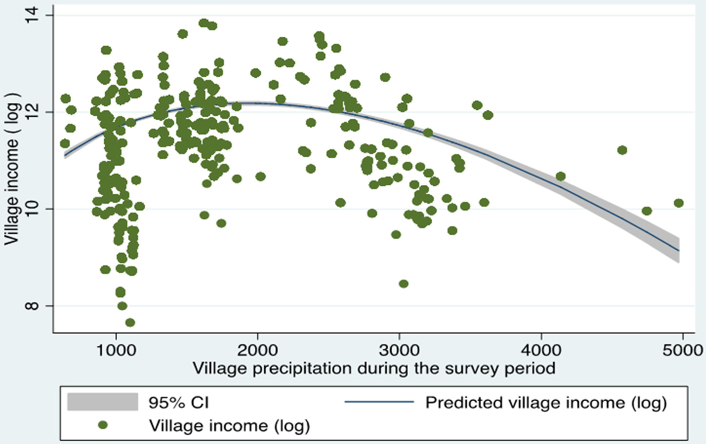
Figure 1. Relationship between rainfall and mean observed village income

Splitting villages into dry and wet zones, we find that the income poor (below the regional median income) households tend to live in dryer villages in the dry area (1,101 versus 1,160 mm/year, t = 14.55), and wetter villages in the wet area (2,280 versus 2,127 mm/year, t = 7.80).

In terms of climate variability, as measured by the standard deviation (SD), the income poor tend to live in villages that experience larger precipitation variability, in both dry (197 versus 180, t = 11.40) and wet (327 versus 277, t = 9.94) areas. The differences are pronounced; for example, poor households in wet areas experience a variation (SD) of rainfall that is 17 per cent higher compared to what rich households experience.

The temperature differences (mean and SD) are smaller and show no systematic pattern across poverty categories.

Overall, the poorest segment of our sample appears to be more exposed to extreme rainfall conditions, both in terms of lower mean rainfall in dry areas and higher mean rainfall in wet areas, as well as higher variability. This is consistent with the findings of Hallegatte et al. (Reference Hallegatte, Bangalore, Bonzanigo, Fay, Kane, Narloch, Rozenberg, Treguer and Vogt-Schilb2015): poor people are relatively more exposed to droughts and – to a lesser extent – floods. Causality could run both ways: extreme climate conditions can reduce income and assets and thus create or deepen poverty, but the least resourceful (asset poor) might also locate themselves in areas with harsher climate conditions, for example, because they cannot afford to buy land in more favorable climates.

4.2.2 Self-reported shocks

Close to a quarter (24 per cent) of the households reported having experienced some type of severe shock during the year covered by the PEN survey (table 6). The income & asset poor have a higher incidence of income shocks compared to the other households (14 versus 9 per cent). In other words, the income & asset poor are > 50 per cent more likely to have experienced a severe income shock. This difference is robust across wet-dry zones and regions. The higher exposure to income shocks among the income & asset poor is consistent with a hypothesis that some asset poor might be in the income & asset poor rather than the income rich & asset poor category due to income loss in the survey year.

Table 6. Shock incidences during survey year across poverty categories

Notes: ** indicate statistical significance at 5%. NS, Not Significant.

^a Kruskal-Wallis test of difference between the groups.

Only small differences are revealed across the other three poverty groups. We expected a higher incidence of (income) shocks among the income poor & asset rich compared with the income & asset rich, i.e., that a higher prevalence of shock could help explain why some asset rich become income poor. This is not the case, possibly because most asset rich households have sufficient means to deal with the shock through income smoothening. Furthermore, most shocks may not be sufficiently large to make the asset rich fall below the income poverty line.

Overall, the findings suggest that income shocks – not unexpectedly – have a negative impact on observed income, and in particular for the asset poor. The results also indicate that the asset rich might have more means to reduce the negative impacts of an income shock, a finding also supported by the coping data below.

4.3 What is the role of environmental income in coping with shocks?

4.3.1 Coping responsesFootnote ¹⁰

The concept of vulnerability encompasses both the sensitivity to harm and the capacity to cope with shocks (IPCC, Reference Mach, Planton, von Stecho, Pachauri and Meyer2014). This paper discusses only the latter.Footnote ¹¹ Table 7 shows how households responded to the three types of shock (income, asset and labor). We include the ‘did nothing in particular’ option. For shocks that reduced income, this response could reasonably be interpreted as ‘did nothing to compensate for the income loss’, i.e., the household lowered consumption and/or reduced savings. Overall, ‘did nothing’ is the most common response (20 per cent). Among the active coping responses, the most frequently mentioned are to take on extra casual (wage) labor (15 per cent) or use household savings (13 per cent), followed by harvest/sell more agricultural products (10 per cent), and harvest more products from forest and other natural habitats (9 per cent).Footnote ¹²

Table 7. Self-reported responses to household shocks by shock type^a

^a Percentage distribution of the highest ranked response.

There is a large and interesting variation in coping strategies across different types of shocks. More wage work is the most common response after an income shock. Spending household savings is the most common one after a labor (including health) shock, which is not surprising as illness prevents the household member from taking up extra work and may involve extra medical expenses. In almost half of the cases of asset loss, the affected household did nothing in particular, possibly because this might not have involved an immediate income loss. Getting assistance from friends, relatives or an organization is much more common after labor shocks, possibly because those tend to be more idiosyncratic than other shocks, and because such shocks involve more social support.

‘Harvesting more environmental products’ as a coping strategy also varies across the different types of shocks. It is ranked second among the responses to income shocks (13 per cent). Among these, this strategy is mentioned more frequently for wage loss than for crop failure, possibly because losing employment frees up family labor that can be used for extractive activities. At the other extreme, harvesting more environmental products is least mentioned as a coping strategy for health shocks, as these reduce the family's labor supply.

To explore how the use of environmental income as a coping mechanism varies among households that experienced a severe shock, we ran a Probit regression model (table 8). Households that are younger and do not have wage income are more likely to obtain more environmental income to cope with shocks. Further, they are more likely to use it when they face an income shock as compared with a labor shock, as also shown in the descriptive statistics. Households living in areas with high rainfall and lower temperature are also more likely to use this coping mechanism, whereas rainfall and temperature variability have no significant impact. Households in Latin America (reference region) are less likely to use harvesting of environmental products as a coping mechanism compared to the three other regions.

Table 8. Probability of using environmental income as a copingmechanism

Notes: Probit regression results. Standard errors clustered at village level. *, **, *** indicate statistical significance at 10%, 5% and 1% levels respectively.

Regarding poverty categories, the income rich & asset poor (stochastically non-poor) are more likely to harvest more environmental products when facing a shock, compared with the income & asset poor (structurally poor). Nineteen per cent of the former group has this as the primary coping strategy as compared to 11 per cent for the latter. Noting that the regression model falls short of being a causal model, but rather estimates partial correlations, a possible interpretation is that households that have access to coping based on environmental resources seem less likely to fall into (or remain in) income poverty when experiencing an income shock. This is consistent with a hypothesis of environmental income serving as a safety net.

The income rich & asset poor is also different from the other groups by having the lowest ‘do nothing’ response (10 per cent compared to 22 per cent for all groups). This group therefore seems to pursue more active coping strategies, either by being more entrepreneurial, by having better access to coping mechanisms (including environmental income), or a combination of the two.

Overall, there is consistent evidence in the literature that the share of environmental income is negatively correlated with total household income, i.e., higher environmental reliance among the poor (e.g., Angelsen and Dokken, Reference Angelsen and Dokken2015). For the safety net role, the results of this paper do not support a hypothesis of environmental income being relatively more important for the income poor as a coping mechanism after shocks. We do find, however, indicators of harvesting environmental products being important for some asset poor households, and it may help them into the income rich & asset poor category, similar to the findings of Ainembabazi et al. (Reference Ainembabazi, Shively and Angelsen2013) and Dokken and Angelsen (Reference Dokken and Angelsen2015). Yet, it is misleading to think of environmental income as ‘quick and easy cash’ in response to a shock. If it was, poor households would not need to be pushed into the forest by a shock to pick valuable and low-hanging fruits.

4.3.2 Forest resources and resource degradation

Given the role forest income plays as a safety net, how does (changes in) the availability of forest resources vary across household categories? As a measure of forest availability, we use tree cover in each of the sampled villages. There are small differences across the different poverty categories, although the income & asset rich tend to live in villages with slightly higher tree cover (table 9), particularly for the sampled households in wet sites in East Asia. In Latin America, the picture is different: forest cover is lower for the income & asset rich. In Africa, where most of the sites are in the dry zones, there is no clear pattern.

Overall, we find limited evidence in support of a hypothesis that the poorest households live in villages with more forests, which then could help them cope with climate (or other) shocks. This finding might be surprising. The forest transition hypothesis (Mather, Reference Mather1992) suggests that forested regions (or countries) might go through distinct stages, from a situation with high forest cover and low deforestation (core forests), to a frontier stage with high deforestation rates, to a stabilization phase with a mosaic landscape. The core forest areas are characterized by poor market access, poorly developed infrastructure and (therefore) relatively high poverty (Chomitz et al., Reference Chomitz, Buys, De Luca, Thomas and Wertz-Kanounnikoff2007; Angelsen and Rudel, Reference Angelsen and Rudel2013). We should therefore expect a negative correlation between household income and forest cover, but find only weak correlations between household income and tree cover within the regions.

We have two possible explanations of this finding. First, there might be some selection bias in the sample, i.e., sampling of high forest cover sites with valuable commercial forest products. Forest income – both absolute and relative – is strongly correlated with forest cover (r = 0.27), and this seems to compensate for the remoteness associated with high forest cover. Second, the forest transition hypotheses does not seem to describe well the pattern in dry forest area in developing countries, but typically has rainforest frontier contexts as its point of reference.

Table 9 also gives the change of tree (forest) cover in the villages during the period 2000–2010, which represents processes of both deforestation and forest degradation. We have no a priori expected signs: high forest loss could signal intensive use and corresponding high forest incomes, but could also indicate degrading resources and shrinking forest incomes.

Table 9. Village tree cover and tree cover change

^a Our definition of forest cover is tree canopy cover within the village (a circle of 5 km radius), and not the standard FAO definition of forest as an area with minimum 10% tree canopy cover. Using that definition would yield significantly higher forest cover figures. Our definition is more suitable for the purposes of this paper, i.e., as a measure of forest resources available.

For the full sample, the income & asset rich have lower rates of forest loss than the other groups, but with large variation across climate zones and regions. In the African sub-sample, the rate of forest loss for the income & asset poor was four times the loss for the income & asset rich.

Any positive correlation between poverty and forest loss is a classic example in which causality could run both ways: do poor people overexploit environmental resources, or does a shrinking resource base make people poor? Fully exploring this issue would preferably use panel data, but the following points are indicative. The strong association between forest loss and structural poverty in the African sub-sample is consistent with the literature on a poverty-environment nexus on the continent (e.g., Duraiappah, Reference Duraiappah1998; Lufumpa, Reference Lufumpa2005). Relatedly, wet forests tend to have more commercially valuable products, timber in particular. This increases both the potential to lift some households out of poverty (cf. the high forest loss among income rich & asset poor in Latin America) and makes forests more attractive to exploitation by outsiders. This might explain the negative association between structural poverty and forest loss in wet areas.