


1 Introduction
Accurately obtaining subjective probabilistic information about uncertain future events is an essential step in the decision making process in many different economic and public policy settings. In many cases, rather than trying to build a model to estimate probabilities, the best and most informative assessments come from an agent who has a good amount of relevant experience and can use her collected wisdom to estimate a subjective probability. Eliciting this information presents an important and difficult problem in many fields such as finance and macroeconomics (Diebold and Rudebusch Reference Diebold and Rudebusch1989; Ghysels Reference Ghysels1993), decision analysis (Keeney Reference Keeney1982), and meteorology and weather forecasting (Murphy and Winkler Reference Murphy and Winkler1984). In addition, probability assessments often comprise an important component of economic experiments. Even when the ultimate objective is not to elicit subjective beliefs, obtaining this information may be a critical secondary step in an experimental procedure.
Well-designed scoring rules provide a useful tool for procuring this subjective information by providing an agent with the right incentives to carefully evaluate and quantify her beliefs, and to honestly reveal her subjective assessment of the likelihood of these uncertain future events. The quadratic scoring rule (QSR), a variant of which was first introduced by Brier (Reference Brier1950), is the most commonly used.Footnote 1
The incentive design of scoring rules implicitly assumes, however, that the agent is risk neutral, which contrasts with how people often behave. Winkler and Murphy (Reference Winkler and Murphy1970) examine the effects of nonlinear utility on the optimal report under a proper scoring rule, showing that risk aversion leads an agent to hedge her reports away from categorical forecasts of 0 and 1 and risk seeking leads the agent to bias her reports closer to 0 or 1. This biasing effect of risk preferences can be easily corrected by applying the inverse utility function to the scoring rule (Winkler Reference Winkler1969). In practice, however, an even more troubling pattern of excessive reports equal to the baseline probability of 1/2 emerges as well, a phenomenon not explained by classical expected utility models. For example, Offerman et al. (Reference Offerman, Sonnemans, van de Kuilen and Wakker2009) tested responses by 93 subjects to a QSR for objective probabilities that ranged from 0.05 to 1 and found that they reported 1/2 more than three times as often as they should have (15.3 % versus 5 %). This particular type of conservatism inhibits the decision maker’s ability to discern among a broad domain of moderate beliefs and conceals a significant amount of useful information.
In this paper, we employ the insights of prospect theory (Kahneman and Tversky Reference Kahneman and Tversky1979; Tversky and Kahneman Reference Tversky and Kahneman1992) to understand the ways in which an agent will distort her report when she receives an uncertain reward from a QSR. Employing Palley’s (Reference Palley2015) model of prospect theory with an endogenous reference point, we highlight how loss aversion can account for why an agent may both report 1/2 for a range of moderate beliefs and bias her reports toward 1/2 for beliefs closer to 0 or 1.
The main contribution of our paper is the introduction of a generalized asymmetric QSR, the L-adjusted rule, which eliminates the incentives for conservative reports and enables the elicitation of true probabilistic beliefs. The payoffs in this L-adjusted rule are the same as in a classical QSR except negative outcomes are shrunk by a factor of L, a parameter that controls the size of the loss adjustment. We use previous experimental work estimating population parameters to derive an off-the-shelf variant of this L-adjusted QSR that requires no prior agent-specific calibration. In an experiment, we demonstrate its effectiveness in recovering truthful and precise probability assessments, and show that it alleviates the shortcomings associated with the classical QSR. In agreement with previous results, we find that in response to the classical QSR, agents tend to report the implicit benchmark probability of 1/2 for a wide range of beliefs near 1/2 in order to ensure a certain payoff. By matching the choice of L to previous empirical estimates of parameters for the overall population, we also obtain a modified QSR that recovers truthful beliefs experimentally. In doing so, we provide a practical and simple off-the-shelf scoring rule that encourages agents to report their beliefs truthfully.
We want to emphasize that the use of the L-adjusted QSR is as easy as the use of a standard QSR. Exactly as with a standard QSR, each subject receives a table that lists how their payoff varies depending their probability judgment and the actual outcome of the predicted phenomenon. The only difference between a standard QSR and an L-adjusted QSR is that the actual payoffs in the table are changed to accommodate subjects’ loss aversion. As a result, subjects are encouraged to automatically report judgments that are very close to true objective probabilities.
The simplicity of our approach depends to a large extent on the fact that we provide each subject with the same L-adjusted QSR based on parameter estimates for the general population. A natural question is how much precision is sacrificed by ignoring differences that may exist in people’s loss-aversion attitudes. To investigate this question, we include a treatment in which we adjust the scoring rule separately for each subject on the basis of an individually estimated loss parameter. Interestingly, we do not find better results for this treatment.
Recently, several related approaches have been suggested to recover true beliefs from conservative reports. Offerman et al. (Reference Offerman, Sonnemans, van de Kuilen and Wakker2009) propose a revealed preference technique that allows the researcher to correct the reported beliefs of agents who are scored according to a standard QSR. In this method, agents initially provide reports for a range of objective probabilities, which then yields an optimal response mapping that can be inverted and applied to infer subjective beliefs from later reports. In an experiment, Offerman et al. demonstrate the effectiveness of this approach in recovering beliefs from reports that do not equal the baseline probability of 1/2. Kothiyal et al. (Reference Kothiyal, Spinu and Wakker2011) extend this method to overcome the problem of discriminating between moderate beliefs in a range around the baseline probability of 1/2, for which agents give the same optimal report. By adding a fixed constant to one of the QSR payoffs, they both eliminate the excess of uninformative baseline reports and yield an invertible response mapping that makes possible the recovery of true beliefs, while maintaining the properness of the original scoring rule. Kothiyal, Spinu, and Wakker do not provide an experimental test of their method.
The approaches taken in Offerman et al. (Reference Offerman, Sonnemans, van de Kuilen and Wakker2009) and Kothiyal et al. (Reference Kothiyal, Spinu and Wakker2011) are precise and elegant because they do not need to make structural assumptions on how people make decisions under risk. The downside of these methods is that they are laborious to employ, because a sufficiently dense risk-correction map has to be derived for each agent before any inferences can be made. In both decision analysis and many experimental economics applications, the elicitation of beliefs is a secondary goal, and a simpler and quicker approach may be preferred, as long as it does not sacrifice precision. The method presented in this paper pursues this purpose.
Other elicitation methods that do not make use of scoring rules exist as well. For example, if the utility function is unknown, Allen (Reference Allen1987) presents a randomized payment method that relies on the “linearization” of utility through conditional lottery tickets to incentivize truthful reports. Alternatively, Karni (Reference Karni2009) proposes a procedure with two fixed prizes where the payment function is determined by comparing the agent’s report to a random number drawn uniformly from [0,1], analogous to the Becker et al. (Reference Becker, DeGroot and Marschak1964) mechanism. Under this method, if the agent exhibits probabilistic sophistication, she has a dominant strategy to report her true belief, irrespective of her risk attitudes. However, in experiments, subjects have been found to have a hard time understanding Becker-DeGroot-Marschak-type procedures (Rutström Reference Rutström1998; Plott and Zeiler Reference Plott and Zeiler2005; Cason and Plott Reference Cason and Plott2012), and empirical comparisons of these methods with scoring rules have yielded mixed results (Hao and Houser Reference Hao and Houser2010; Hollard et al. Reference Hollard, Massoni and Vergnaud2010; Trautmann and van de Kuilen Reference Trautmann and van de Kuilen2011).
The rest of the paper is organized as follows: Sect. 2 introduces our L-adjusted QSR and characterizes the corresponding optimal reporting policy under the prospect theory model of risk behavior. We discuss how this predicted behavior provides a parsimonious explanation of previously observed conservative reporting patterns and how the parameter L can be calibrated to allow for the recovery of estimates of any probabilistic belief. Readers who are interested mainly in how well our method encourages subjects to simply report true probabilities may skim Sect. 2 and refer to Proposition Footnote 1 and Corollary Footnote 1. Sections 3 and 4 detail the experiment that we carried out to test the usefulness of this adjusted scoring rule in practice and demonstrate its improvements over the classical QSR. Section 5 concludes and Appendix 1 characterizes reporting behavior for the general asymmetric L-adjusted QSR and contains proofs of all results. Appendix 2 in Supplementary Material provides images and instructions from the experimental interface.
2 The model
We consider an agent who must report a subjective belief about the chances of an uncertain future event
 . Her true belief is that event
 will occur (
 ) with probability
 and its complement
 will occur (
 ) with probability
 . She submits a reported probability
 that
that
 will occur and receives a payoff according to an L-adjusted QSR, a generalization of the asymmetric QSR introduced by Winkler (Reference Winkler1994).
Definition 1
(L-adjusted Quadratic Scoring Rule) The L-adjusted asymmetric QSR is defined by
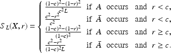
In general, the L-adjusted QSR can be centered around any baseline probability
 of the event
 occurring,Footnote 2 but for most of the paper we will focus on the typical case of a symmetric baseline
 . When
 this scoring rule reduces to the asymmetric QSR and when
 and
and
 it reduces to the classical binary QSR.
The pattern of reporting behavior that previous studies have observed cannot be explained by classical expected utility theory. Therefore, to understand how an agent will respond to this risky payoff function, we apply a prospect theory model of risk preferences. Prospect theory applies psychological principles to incorporate several important and frequently observed behavioral tendencies into the neoclassical expected utility model of preferences. This more flexible formulation provides a useful descriptive model of choice under risk (Camerer Reference Camerer, Camerer, Loewenstein and Rabin2000) and generally includes four main behavioral components:
1. Reference Dependence The agent evaluates outcomes as differences relative to a reference point rather than in absolute levels.
2. Loss Aversion Outcomes that fall below the reference point (“losses”) are felt more intensely than equivalent outcomes above the reference point (“gains”).
3. Risk Aversion in Gains, Risk Seeking in Losses, and Diminishing Sensitivity to Both Gains and Losses The agent tends to prefer a sure moderate-sized outcome over an equal chance of a large gain or zero gain, but prefers an equal chance of taking a large loss or avoiding the loss altogether over a sure moderate-sized loss. In addition, the marginal effect of changes in the outcome for the agent diminishes as the outcome moves away from the reference point.
4. Probability Weighting The agent overweights probabilities close to 0 and underweights probabilities close to 1.
Of critical importance in applying prospect theory to model choices under risk is the determination of the reference point. Often the reference point is implicitly set to equal 0, but this assumption may not be realistic when all outcomes are positive, as is typical in practice when rewarding subjects for providing reports according to a QSR. For example, if the reference point were taken to be 0, then all outcomes in our experiment would be viewed as “gains” and the prospect theory model would be unable to explain the observed reporting behavior.
Instead, we argue that even in settings where all outcomes are nominally positive, an agent may still feel elation or disappointment based on whether the payoff she receives falls above (a “gain”) or below (a “loss”) what she expected at the time that she submitted her report. To model this, we assume that the agent possesses a reference-dependent utility function of the form of Palley (Reference Palley2015), in which the agent develops an expectation
 about her outcome
 from the scoring rule, and this expected outcome then forms a natural reference point for her to evaluate the outcome that she ultimately receives. This utility function extends existing models of an endogenously determined reference point (see, e.g., Shalev (Reference Shalev2000)) to accommodate the case of an agent with prospect-theory-type preferences. This model will provide a parsimonious explanation for the behavior that is observed, and most importantly, can be readily used to provide a solution to the problem and insight into why it works.
Specifically, we assume that when the agent’s outcome exceeds this expectation, she feels an additional gain of
 , where
 specifies the curvature of her risk preferences. When her outcome falls below her expectation, she perceives this as an additional loss equal to
 , where
 additionally parameterizes the agent’s degree of loss aversion. Mathematically, this utility function is specified by
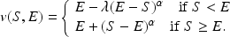
If
 , this formulation coincides with the loss-averse utility function detailed in Shalev (Reference Shalev2000). If
 , then this simplifies to the risk-neutral objective of maximizing expected payoff that the definition of a proper scoring rule implicitly assumes.Footnote 3
In addition, we assume that the agent applies probability weighting functions
 and
and
 for scores that fall above and below
 (positive and negative events), respectively.
 and
and
 are assumed to be strictly increasing with
 ,
,
 , and
, and
 for all
 .Footnote 4 The ex ante expected-valuation that an agent receives from responding to a binary scoring rule is then given by a probability-weighted sum over the possible scores;
 Footnote 5
Until this point, we still have not specified the details of how the reference point
 is determined. The motivating intuition we follow here is that the agent’s expected-valuation of the prospect should be consistent with her expectation about the prospect. In other words, if she uses
 as her reference point in determining
 , then the resulting expected-valuation should simply equal
 itself. Specifically, we assume that the reference point
 is determined endogenously according to the consistency equation
 , as in Palley (Reference Palley2015). In this sense, for a given prospect, a consistent reference point
 is the expectation that perfectly balances the agent’s potential gains against her potential losses, weighted according to her beliefs of their respective likelihoods.
A consistent reference point
 is the natural evaluation of a prospect for an agent who carefully contemplates the possible outcomes and anticipates her possible ex post feelings, providing a summary measure of how the agent evaluates the risk in an ex ante sense. An agent who initially forms a reference point
 higher than
 will find that her expected losses
 outweigh her expected gains
 , causing her to adjust her expectation downward.
Conversely, an agent whose reference point is initially lower than
 will find that her expected gains outweigh her expected losses, causing her adjust her reference point upward. A thoughtful agent will thus converge to a unique consistent expectation
 . This notion of expectations as an endogenously determined reference point is introduced and developed in the models of Bell (Reference Bell1985), Loomes and Sugden (Reference Loomes and Sugden1986), Gul (Reference Gul1991), Shalev (Reference Shalev2000), and Koszegi and Rabin (Reference Koszegi and Rabin2006, Reference Koszegi and Rabin2007).
Note that the relationship between the reference point and the valuation function possesses an intentional “circularity,” which is an important part of the model. For any prospect, there exists only one unique reference point E that satisfies V(E) = E, and this is the reference point that represents the agent’s ex ante valuation of a given prospect. It is this equation that ensures the consistency of the valuation function and the reference point, and which pins down the appropriate expectation E.
Figure 1 displays an example of this reference point formation process. We see that a loss-averse agent with subjective beliefs of
 would derive an ex ante expectation of
 from truthfully reporting
 in response to a QSR, while deriving an ex ante expectation of
 from reporting
 . Both of these reports are therefore dominated by reporting the baseline
 , which yields an outcome of 0 with certainty and a corresponding ex ante expectation of
 . Whereas a risk-neutral agent would prefer to report
 , which yields the highest expected score, the loss-averse agent in this case will prefer to report
 .
.
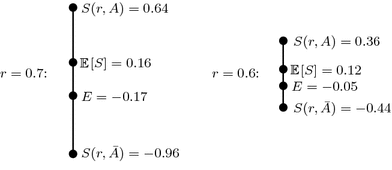
Fig. 1 Two examples of an agent’s possible report choices and corresponding ex ante reference point formation in response to an classical QSR with baseline
 when the agent believes the probability of event
 is
is
 , has prospect theory parameters
 and
and
 , and does not apply probability weighting
We assume that the agent seeks to maximize her expected outcome
 over all possible reports
 , subject to the consistency requirement, which essentially means that the agent will consider her ex post prospects when she chooses her report and forms her ex ante expectation about her outcome. The timeline of events is displayed in Fig. 2.
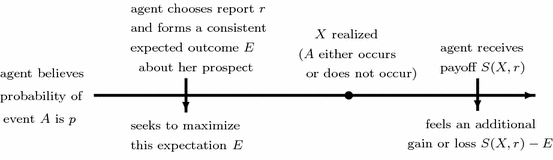
Fig. 2 Timeline of the agent’s report choice, reference point formation, and ex post evaluation of the event
Proposition 1
The optimal consistent report function when
 is given by
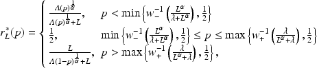
where
 is the agent’s loss-weighted odds ratio of event

The optimal consistent response function for more general (asymmetric) baseline probabilities
 can be found in Appendix 1.Footnote 6
Proposition 2
For any positive linear rescaling of the payoffs
 ,
,
 , the optimal consistent report remains
 and the corresponding optimal
ex ante
expected outcome is rescaled according to
and the corresponding optimal
ex ante
expected outcome is rescaled according to
 .
.
In other words, in contrast to the predictions of the cumulative prospect theory model with a fixed reference point and many classical utility formulations, the agent’s behavior will be invariant to positive linear rescaling of the payoffs. This means, for example, that the agent’s optimal behavior would not change if the decision maker decided to pay her in a different currency with exchange rate
 :1 or pay her an additional fixed fee
 for providing the report.
Figure 3 displays the shape of optimal reports as a function of the agent’s beliefs
 in response to the classical QSR. For a large region of moderate beliefs near
 , the agent will prefer to simply report
 in order to receive a payoff of
 with certainty. While the width of this region depends jointly on
 ,
,
 ,
,
 , and
, and
 , it is largely driven by the loss aversion parameter
 . The shape of the optimal consistent report function closely mirrors the theoretical results of Offerman et al. (Reference Offerman, Sonnemans, van de Kuilen and Wakker2009). Here the decision maker cannot simply provide the agent with the classical QSR and then infer her true beliefs from her report because the resulting response function
 is not invertible. All beliefs
 in the interval
 are mapped to the conservative risk-free report of
 (this is the flat region of the optimal report function). This means that observing a report of
 , which may happen quite frequently if the agent is loss-averse and has moderate beliefs, tells the decision maker only that the agent’s beliefs lie somewhere within that interval.
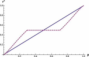
Fig. 3 Optimal consistent report
 (the dashed line) to the classical QSR (
 ,
,
 ) for
) for
 ,
,
 , and
, and
 versus truthful reporting (the solid line)
2.1 Determining the
 -adjustment

To recover true beliefs, the decision maker needs to instead adjust the scoring rule to eliminate the “flat region” of conservative reports of
 , which will allow him to invert the agent’s optimal report function
 and estimate
 according to
 . Sensitivity analysis suggests that loss aversion accounts for the largest proportion of this conservative behavior. The best way to counteract this phenomenon, then, is to adjust the scoring rule so that negative outcomes are less severe by a factor of
 . By computing the value
 that solves
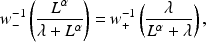
the decision maker can squeeze the endpoints of the “flat region” of conservative reports of
 together and recover the agent’s true beliefs.
Corollary 1
The optimal adjustment when
 is given by
This calibration of
 eliminates the agent’s incentive to provide these uninformative reports even for very moderate beliefs close to
 , and also removes almost all of her distortion in the optimal reporting function. After receiving her report, the decision maker can apply the inverse of the optimal report function to the observed report
 to recover the agent’s exact truthful beliefs
 . In the absence of utility curvature and probability weighting (
 and
and
 ), the optimal adjustment is simply equal to the loss aversion parameter (
 ) and the inversion step is unnecessary because the optimal report function is truthful (
 ).
).
In practice, an agent’s report may include a noisy error term
 , so that the agent reports
 instead. This means that the inferred beliefs will also contain an error of
 However, since
 is differentiable and close to the identity function for a broad range of reasonable parameter values, the resulting error in inferred beliefs simply scales roughly equally to the size of the original reporting error. Another concern with the L-adjustment method is that it may become laborious if agents are very heterogeneous. In such a setting, the model parameters
 ,
,
 , and
, and
 and the corresponding
 would have to be estimated individually. Our experimental results show, however, that heterogeneity is only of secondary importance and that our method does a remarkable job even without a correction of individual differences.
Figure 4 displays the optimal reports in response to an L-adjusted scoring rule, which is calibrated to average parameter estimates
 ,
,
 ,
,
 ,
,
 ,
,
 and
and
 (yielding
 ) from the studies discussed in footnotes 4 and 5 for the general population, for an agent with various actual loss aversion parameters
 , utility curvature parameters
 , and both with and without probability weighting. As might be expected, given that the adjustment is primarily designed to address distortions due to loss aversion, optimal report functions are most sensitive to misestimation of the parameter of loss aversion
 , and are less sensitive to variations in
 and the probability weighting functions. This suggests that if the decision maker does not want to assess individual parameters, the most important measurement to focus on is
 . We also see that if
 is miscalibrated due to errors in parameter estimates, he may observe reports both above and below the true beliefs
 , depending on whether the
 estimate is too high or too low.
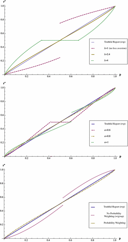
Fig. 4 Optimal consistent reports
 in response to the L-adjusted QSR with
 and
and
 when
when
 ,
,
 ,
,
 ,
,
 ,
,
 and
and
 versus truthful reporting (the solid line). The upper graph considers varied values of
 , keeping the other parameters fixed. The middle graph considers varied values of
 , keeping the other parameters fixed. The lower graph considers the cases of probability weighting and no probability weighting, keeping the other parameters fixed
Next, note that any remaining difference between the optimal report function in response to the
 -adjusted rule and truthful reporting, which in theory could be corrected by applying
 to the observed report, would be completely swamped by any noise in reports and the distortionary effects of errors in the parameter estimates. As a result, in practice there is very little benefit to attempting to carry out this second inversion step on the reports
 . A more practical approach is to simplify the assessment process by eliminating this second inversion step and taking the reported probability as our estimate of the agent’s true beliefs. In doing so, the decision maker should keep in mind the remaining potential for distortion, which is mainly caused by incorrect estimation of the agent’s parameters, and understand that her reports may be somewhat noisy due to this miscalibration.
If the decision maker wishes to avoid the potentially laborious process of individually assessing parameter values for each agent beforehand, a simple approach is to simply present the agent with the L-adjusted QSR with
 and take her resulting report as the estimate of her true beliefs. If the decision maker does want to spend some time and effort to estimate the agent’s parameter values ahead of time, he should focus on accurately assessing her loss-aversion parameter
 , since this offers a fair amount of flexibility in calibrating the scoring rule, and variation in the other parameter values has a less significant effect on the optimal report function.
Below we outline a simple approach that the decision maker can use to estimate
 and
and
 on an individual basis: first, assume that the agent’s utility curvature is
 and probability weighting function is
 . This implies that for a 50–50 lottery between receiving
 and
and
 , where
 , her consistent expectation is given byFootnote 7

Next, the agent is offered a choice from a carefully designed set of coin flips that offer different payoffs depending on whether the coin ends up heads or tails. We assume that the agent makes this choice so that she maximizes the consistent expectation given in Eq. 2, meaning that she will prefer different lotteries for different values of
 . Specifically, the set of coin flips offered is designed so that each lottery is the most preferred option for a specific interval of possible
 values. Once the agent selects her most preferred lottery from this set, the decision maker can use her choice to make inferences about her loss aversion parameter, for example, by taking the midpoint of the interval of
 values for which that flip is the most preferred. As noted in the discussion of Corollary Footnote 1, under these assumptions, the optimal
 -adjustment is then simply equal to that
 estimate. An example of such a set of coin flip lotteries and the
 parameters implied by each can be found in the description of the IC treatment in Sect. 3.
3 Experiment
Offerman et al. (Reference Offerman, Sonnemans, van de Kuilen and Wakker2009) show that, in practice, proper scoring rules fail to elicit truthful reports from human agents, with patterns of reporting behavior that match the theoretical model of this paper. In this experiment we confirm the predictions of the preceding theory and demonstrate the feasibility of the L-adjusted scoring rule in recovering truthful beliefs from human subjects. In doing so, we demonstrate that the L-adjusted rule provides a simple modification of the QSR that can be used for most agents to obtain relatively accurate reports from the general population without having to arduously assess individual parameter and curvature estimates. In addition, we test several values of
 and show that the proposed rescaling
 is indeed the most effective at eliciting truthful beliefs from agents.
3.1 Experimental design and procedures
The computerized experiment was carried out at the CREED laboratory of the University of Amsterdam. Subjects were recruited from the undergraduate population using the standard procedure, with a total of 183 subjects participating in the experiment. Subjects earned on average 13.00 euros (€) for an experiment that lasted approximately 35 min. Subjects read the instructions on their screen at their own pace. After finishing the instructions, they had to correctly answer some control questions that tested their understanding before they could proceed to the experiment. Subjects also received a handout with a summary of the instructions before beginning the experiment (Appendix 2 in Supplementary Material provides a sample of the instructions).
We employed a between-subjects design, in which each subject participated in exactly one of four treatments. The first three treatments differed only in the size of the loss correction applied to the QSR. In the control treatment we used
 , which therefore corresponds to the classical QSR that has been previously employed in many experiments. We refer to this treatment as NC (mnemonic for no correction). In treatment medium correction (MC), we applied a moderate-sized correction of
 and in treatment large correction (LC) we applied the large loss correction of
 derived and predicted to be optimal in Sect. 2.1.
In each of these three treatments, subjects were informed that the experiment would last for 20 rounds and that at the end of the experiment one of the rounds would be randomly selected and used for actual payment. In each round, a subject was asked to give a probability judgment that a randomly drawn number from the set
 would be in the range
 . The randomly drawn number was an integer and subjects knew that each number in the set
 was equally likely. The range was given at the start of a round and differed across rounds. The lower bound of the range was 0 and the upper bound, which determined the true objective probability, differed across rounds. In the 20 rounds we used the
 values
 , in a random order. For example, in the round that used
 , the subject was asked to give the probability judgment that the randomly drawn integer would fall in the set
 . While the subject was free to report any probability that he or she wanted, the objective probability of this event is given by
 , so in the example of
 the true probability was
 . Each subject was presented with the ranges in a random order to prevent the possibility that order effects might confound the results. Subjects did not receive any feedback between successive rounds, so there was no opportunity to learn from previous rounds.
Subjects were given a handout with a tabular depiction of the L-adjusted QSR that pertained to their treatment. The table clarified how their possible payoffs would change depending on what probability they reported. The scoring rules were in units of euros rescaled by a factor of 3 and shifted upward by 12, so that payments ranged between a minimum of €3 and a maximum of €15, and participants could assure themselves a payoff of €12 by always reporting
 .
.
Appendix 2 in Supplementary Material includes the three payoff tables that we used in the experiment. When a subject had tentatively decided which report
 he or she wanted to provide in a given round, they were asked to type this probability judgment into a box on the upper part of the screen. Once this response was entered, the lower part of the screen then automatically displayed the relevant part of the payoff table with the current decision highlighted. Using arrows, subjects could scroll through the payoff table and if they desired, increase or decrease their report until they settled upon an ultimate response. Their choice was not finalized until they clicked the button “Satisfied with choice” (Appendix 2 in Supplementary Material shows the decision screen). After a subject had provided all 20 responses, the computer randomly selected exactly one round (indexed by the upper bound of its range
 ), which then determined his or her payment as follows: first, the computer drew a random integer from the set
 and determined whether the number was in the range
 of that round or not. Second, the payoff was determined by inputting both the realization of whether the number was in the range or not and the subject’s probability judgment
 for that round into to the scoring rule that the subject had faced. At the end of the experiment subjects filled out a questionnaire and were privately paid their earnings.
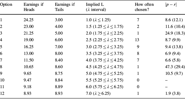
In the fourth treatment we provided each subject with an individually calibrated L-adjusted rule.Footnote 8 We included this treatment individual correction (IC) to investigate how much precision was lost by correcting each subject with the same L-adjusted QSR. The uniform loss corrections that we use in MC and LC may not work well when subjects differ substantially in their loss-aversion attitudes. Treatment IC consisted of two parts: At the start, subjects were informed that they would make 21 decisions in total, 1 in part 1 and 20 in part 2, and that at the end of the experiment one of these 21 decisions would be selected at random for actual payment. While making their decision for part 1, subjects did not yet have access to the instructions of part 2. In part 1, each subject chose one of the 12 options listed in Table 1. Subjects were told that if this decision were selected for payment, their chosen option would determine their payment together with the outcome of a random coin toss by the computer. If the coin flip came up heads (tails), then the payoff in the second (third) column would apply.
Table 1 Individual assessment of the loss-aversion parameter
 (part 1 of treatment IC)
|
Option |
Earnings if Heads |
Earnings if Tails |
Implied L (
|
How often chosen? |
|
|---|---|---|---|---|---|
|
1 |
24.25 |
3.00 |
1.0 (
|
7 |
8.6 (12.1) |
|
2 |
23.00 |
4.00 |
1.5 (
|
2 |
11.6 (10.4) |
|
3 |
21.25 |
5.00 |
2.0 (
|
1 |
24.9 (18.3) |
|
4 |
19.00 |
6.00 |
2.5 (
|
13 |
8.7 (9.9) |
|
5 |
16.25 |
7.00 |
3.0 (
|
9 |
9.4 (13.8) |
|
6 |
13.00 |
8.00 |
3.5 (
|
8 |
6.9 (9.4) |
|
7 |
11.50 |
8.40 |
4.0 (
|
7 |
6.6 (5.8) |
|
8 |
10.65 |
8.60 |
4.5 (
|
1 |
47.3 (29.4) |
|
9 |
9.65 |
8.75 |
5.0 (
|
1 |
10.5 (9.7) |
|
10 |
9.47 |
8.84 |
5.5 (
|
0 |
– |
|
11 |
9.18 |
8.89 |
6.0 (
|
0 |
– |
|
12 |
8.93 |
8.93 |
7.0 (
|
1 |
1.9 (3.8) |


The left 3 columns list the options between which the subjects in part 1 of treatment IC were asked to choose; earnings are denoted in euros. The fourth column lists the L-parameter implied by a choice. The fifth column lists how often each option was chosen and the final column lists, for each option, subjects’ average absolute deviations of the reported probabilities
 from the true probabilities
 (as determined by the range
 according to
 ), with the standard deviations in parentheses
The fourth column of Table 1 lists the L parameter implied by a subject’s choice (this was not observed by our subjects). After part 1, subjects proceeded with part 2, which was the same as in the other three treatments, except for the fact that each subject was provided with their own individual L-adjusted scoring rule corresponding to their choice in part 1. The 12 possible payoff tables for these L-adjusted QSRs are included in Appendix 2 in Supplementary Material.
We ran two separate sessions for each treatment. In total, 45 subjects participated in NC, 42 subjects in MC, 46 subjects in LC, and 50 subjects in IC.
4 Experimental results
We start with a brief description of the individual differences in treatment IC listed in Table 1. In part 1, 74 % of the subjects chose options that correspond to moderate L parameters in the range
 . The most common deviation was for subjects to behave risk-neutrally and choose option 1; 14 % of our subjects behaved in this way. The final column of Table 1 displays the absolute difference between reported and true probabilities, averaged for all individuals who chose the same option in part 1. Interestingly, there is no clear relation between a subject’s implied L parameter and the average absolute deviation of the reports from the true probabilities. Subjects with large loss adjustments can be corrected roughly as well as subjects with small loss adjustments.
Figure 5 provides an overview of the results by graphing the average reported probabilities in each treatment as a function of the true objective probability
 . The solid black line presents the ideal report function of correct objective probabilities
 . The control treatment NC displays a commonly observed pattern for data collected with uncorrected scoring rules. Subjects overwhelmingly bias their reports in the direction of risk aversion by reporting probabilities that are closer to 50 % than the true probabilities. In the treatment with a medium correction MC, subjects’ these differences are substantially diminished compared to the control treatment, but a systematic bias in the direction of risk aversion still survives. The treatment with individual corrections IC provides on average the same results as MC when the true probability is below 50 % but better results for true probabilities above 50 %. However, under the treatment with a large loss correction LC, the systematic bias vanishes and the average reported probabilities are almost identical to the true probabilities across the whole range of
 .
.
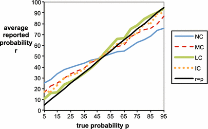
Fig. 5 Average reported probability function
 for each treatment versus the true objective probability report
 . Note that probabilities in the graph are written in percentage terms (% from 0 to 100) rather than decimal units (0–1)
A good elicitation method not only avoids systematic biases but also minimizes variance in the reported probabilities, so that reports will be both honest on average and relatively precise, meaning that a typical deviation from the honest report will not be too large. Figure 6 provides a more detailed view of reports in each treatment by adding standard deviations above and below the average reported probabilities. For treatments NC and MC, the standard deviation is smallest for the true probability of 50 % and increases proportionally with the distance between the true probability and 50 %. The picture is somewhat different for treatments LC and IC, in which the standard deviation gradually diminishes as the probability increases. Figure 7 displays the median reports in each treatment, which provides another perspective of the ‘typical’ behavior under each treatment. We can see that median reports in the control treatment NC display a wide flat region of uninformative reports near
 that is predicted by the preceding theory. This characteristic flat region, which is highlighted more readily by the computation of the proportion of 50 % reports in Table 2 below, is masked in the graphs in Fig. 6 because the underlying flat region is averaged against more extreme reports.
Table 2 Comparison between treatments

|
Treatment |
|
|
Spearman Rank
|
Frequency of 50 % reports |
Frequency of 50 % reports for p = 45 %, p = 55 % |
Risk Bias |
|---|---|---|---|---|---|---|
|
NC |
12.9 (11.8) |
305.9 (524.5) |
0.75 |
39.8 % |
62.2 % |
12.0 (13.3) |
|
MC |
8.5 (10.1) |
173.7 (358.1) |
0.87 |
23.5 % |
39.3 % |
5.7 (12.3) |
|
LC |
7.9 (10.9) |
180.9 (541.2) |
0.92 |
10.1 % |
22.8 % |
−1.0 (13.5) |
|
IC |
9.4 (12.8) |
252.0 (833.6) |
0.84 |
16.0 % |
24.0 % |
3.9 (15.7) |
|
Mann-Whitney probability |
||||||
|
NC versus MC |
0.00 |
0.01 |
0.02 |
0.02 |
0.02 |
0.00 |
|
NC versus LC |
0.00 |
0.00 |
0.00 |
0.00 |
0.00 |
0.00 |
|
NC versus IC |
0.01 |
0.01 |
0.13 |
0.00 |
0.00 |
0.00 |
|
MC versus LC |
0.43 |
0.46 |
0.58 |
0.01 |
0.06 |
0.00 |
|
MC versus IC |
0.86 |
0.88 |
0.46 |
0.15 |
0.10 |
0.21 |
|
LC versus IC |
0.33 |
0.37 |
0.20 |
0.26 |
0.70 |
0.01 |


Probabilities in the table are written in percentage terms (% from 0 to 100) rather than decimal units (0–1). Each cell lists the average for the relevant statistics, with the standard deviations in parentheses.
 denotes the true probability (determined by the range
 according to
 ) and
) and
 denotes the reported probability. ‘Frequency of 50 % Reports for p = 45 %, p = 55 %’ denotes the relative occurrence of 50 % reports when the true probability equals 45 or 55 %. Risk bias equals
 if
if
 , and equals
 if
if
 (cases where
 are excluded). Mann-Whitney tests use average statistics per subject as data points (45 subjects in NC, 42 subjects in MC, 46 subjects in LC, and 50 subjects in IC). In the text, the threshold for significance is at the 5 % level
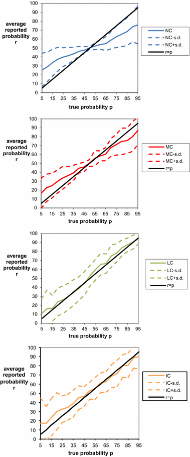
Fig. 6 Average reported probability function
 with
with
 one standard deviation for each treatment versus the true objective probability report
 . Note that probabilities in the graphs are written in percentage terms (% from 0 to 100) rather than decimal units (0 to 1)
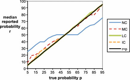
Fig. 7 Median reported probability function
 for each treatment versus the true objective probability report
 . Note that probabilities in the graph are written in percentage terms (% from 0 to 100) rather than decimal units (0 to 1)
Table 2 compares the performance of the treatments with respect to six measures. First, for each subject we computed the average absolute difference between the reported and true probabilities. Both treatments MC and LC that apply a loss correction perform substantially better than the control treatment without such a correction, with absolute errors roughly halved. Mann-Whitney tests that use average statistics per subject as data points reveal that the differences between MC and NC and between LC and NC are both significant. Thus, in both treatments where a uniform loss-correction is applied (MC and LC), subjects’ reported probabilities are systematically closer to the actual probabilities than without a loss-correction (NC). Treatment LC performs on average somewhat better than MC, but this difference is not significant. Surprisingly, treatment IC produces on average somewhat worse results than LC and MC, but the differences are far from significant. Like MC and LC, IC yields a clear and significant improvement compared to NC.
A similar picture emerges for our second error measure, which is based on subjects’ average squared differences between reported and true probabilities. Again, the MC, LC, and IC treatments substantially and significantly outperform the control treatment NC, and while LC additionally seems to do a somewhat better job than MC and IC, the latter differences are not significant.
As a third measure, we computed the Spearman rank correlation between reported and true probabilities for each subject. Ideally, a belief elicitation measure would elicit beliefs that perfectly correlate with true probabilities. In studies that employ uncorrected scoring rules, it is well known that a few subjects are very much attracted by the sure payoff corresponding to a report of 50 %, which results in a poor correlation between reported and true probabilities. Table 2 shows that indeed MC and in LC produce substantially and significantly higher Spearman rank correlation coefficients than NC does. Likewise, IC also yields a clearly larger correlation than NC, but this difference fails to reach conventional significance levels. The differences between MC, LC and IC are again insignificant.
As a fourth measure, we compare the treatments to the extent that they induce uninformative 50 % reports. If subjects were to always report true probabilities, reports of 50 % should occur in only
 th of the cases. NC and MC substantially overshoot this ideal benchmark, with frequencies of 50 % reports equaling 39.8 and 23.5 %, respectively. In comparison, IC and in particular LC perform very well, producing such reports only 16.0 and 10.1 % of the time, respectively. All pairwise differences between the treatments are significant with respect to this frequency of 50 % reports, except the one between MC and IC and the one between LC and IC.
The fifth measure focuses on the frequency of uninformative 50 % reports when the true probability equals 45 or 55 %. As explained in Sect. 2, loss corrections are expected to matter most for such true probabilities close to 50 %. In agreement with the theoretical arguments, the difference in the frequency of reports of 50 % is particularly large in this category. NC and MC perform especially poorly with respect to this benchmark, with frequencies of 50 % reports equaling 62.2 and 39.3 %, respectively. Again, LC and IC do a much better job in comparison; in these treatments, such reports occur only 22.8 and 24.0 % of the time, respectively.
Finally, our sixth measure makes precise the extent to which the three treatments suffer from systematic risk biases. For each subject, we computed how much on average a subject biased the report in the direction of 50 %. If the average risk bias is positive (negative) then this provides evidence that subject are risk averse (risk seeking). Consistent with Fig. 6, the final column of Table 2 shows that subjects are very biased in the direction of risk aversion in treatment NC. In treatments LC and IC, there is almost no bias, and the bias in treatment MC falls roughly in the middle of the other treatments. All risk bias differences between the treatments are highly significant, except the one between MC and IC.
Figure 8 shows how average absolute errors
 in the report vary with the objective probability
 in each of the treatments. The uncorrected scoring rule performs well precisely where we would expect it to—the incentives to make a conservative baseline report of 50 % impel almost unanimously honest reporting when the objective probability is in fact very close to 50 %. However, the uncorrected scoring rule performs far worse than the loss-corrected scoring rules when the true probabilities are larger than approximately 65 % or smaller than approximately 35 %. In other words, errors in the uncorrected scoring rule occur exactly in cases where the effects of loss and risk aversion kick in most heavily. Overall, the uncorrected scoring rule thus proves to be unreliable for eliciting subjective beliefs, since the decision maker does not know which of these regions the true probability belongs to.
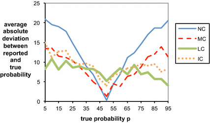
Fig. 8 Average absolute error
 in the reported probability function
 for each treatment. Note that probabilities in the graph are written in percentage terms (% from 0 to 100) rather than decimal units (0–1)
Figure 9 displays the empirical density of the Spearman-rank correlation coefficients in the three treatments. In all treatments most subjects have fairly high Spearman-rank correlation coefficients larger than 0.9, while a few subjects have very low coefficients smaller than or equal to 0.5. The treatments differ primarily in the relative frequency of these two categories of correlation coefficient (high or low). The proportion of overly cautious or haphazard reporters with a low coefficient of less than or equal to
 equals 20.0 % in NC, 14.0 % in IC, 7.1 % in MC and only 2.2 % in LC.Footnote 9
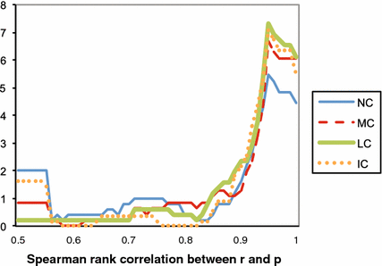
Fig. 9 Histogram of the Spearman-rank correlation (SRC) between the true probabilities
 and the subject’s reported probabilities
 . The figure displays for each SRC the percentage of subjects that fall in the interval [SRC − 0.05, SRC + 0.05]. The few observations where SRC < 0.5 are added to SRC = 0.5
5 Discussion
In practice, quadratic and other proper scoring rules can fail to recover the true probabilistic beliefs that they are designed to elicit. Distortions in agents’ reports generally take one of two forms: first, a risk-averse agent may bias her report away from categorical beliefs of
 and
and
 , as predicted by, for example, the theory of Winkler and Murphy (Reference Winkler and Murphy1970). Second, a risk-averse agent with moderate beliefs close to the baseline probability of
 may revert to simply reporting
 in order to receive a risk-free payoff. In other words, under proper scoring rules such as the classical QSR, we should expect to see a large proportion of uninformative reports of
 , and even strong beliefs near
 or
or
 will be skewed toward this focal point of
 . This pattern of conservative behavior, which has been observed experimentally by, for example, Offerman et al. (Reference Offerman, Sonnemans, van de Kuilen and Wakker2009) and in the experiment of this paper, is explained by the prospect theory model in Sect. 2 of this paper.Footnote 10
The predictions of this theory reinforce the existing result that agents may not reveal their true beliefs even when assessed by a proper scoring rule, and provide an explanation for when and why we might expect to see these two forms of distortions. As demonstrated in Sect. 2, both effects appear to be largely driven by loss aversion, which motivates the agents to seek a certain payoff when they have moderate beliefs and to lower their risk by generally shading their reports closer toward
 for stronger beliefs. The intuition here is that reporting something other than
 introduces uncertainty into the payoffs, so that some outcomes will be felt as gains and some outcomes will be felt as losses. As a result, a loss-averse agent with beliefs close to
 (who doesn’t have much better information than the default baseline prediction) will not find it worthwhile to expose herself to the possibility of these losses. The L-adjusted QSR, which generalizes the classical QSR, can be calibrated to correct for both forms of distortions predicted by this prospect theory model of optimal reports. The
 -adjusted QSR provides a simple scoring rule that can be used in a straightforward manner to elicit an agent’s true subjective probabilistic beliefs. The main challenge in successfully implementing this rule is that the optimal choice of
 requires an accurate estimate of the agent’s parameters
 ,
,
 , and
, and
 . In particular, when applying this adjustment the decision maker needs to be careful not to use an unsuitable value of
 . For example, an agent who is truly risk neutral will respond to an
 -adjusted scoring rule by biasing her reports away from
 for any choice of
 .
.
Our experimental results demonstrate that the biases in people’s reports respond to the adjusted QSR as predicted by the theory. Our data suggests that the optimal calibration of
 for the average population does indeed perform better than the other treatments, but even the moderate-sized correction of
 provides a vast improvement over the classical unadjusted QSR. The major potential benefits of this
 -adjustment include eliminating the flat region of reports
 for moderate beliefs, which are uninformative and prevent the optimal report function from being inverted, and de-biasing reports, so that they provide truthful subjective beliefs on average.
In theory, when processing reports, an decision maker would need to implement an additional second step of computing
 and inferring true beliefs according to
 rather than simply using the raw report
 as the estimate. In practice, however, the impact of this additional step will be very small and likely dwarfed by noise in the reports and errors in the calibration of
 to the agent. Our experiment confirms that the second step is indeed unnecessary, and that reports can be simply recorded as provided in a straightforward manner.
For the general population,
 does seem to be the best adjustment to use, as predicted by applying existing empirical estimation of population parameters to our theoretical results and as evidenced in our experiment. Importantly, a more laborious procedure in which we provide each subject with an individually calibrated L-adjusted rule produces slightly worse results. The difference in performance is small though, and far from significant. One possible explanation is that we did not estimate subjects’ loss aversion parameters with sufficient precision. An avenue for future research is to try to improve the results of the IC treatment by estimating a subject’s loss-aversion parameter on the basis of a series of choices. Our conjecture is that the potential benefits of such an approach are limited. As the results of our paper indicate, no systematic risk bias remains when subjects are adjusted with the
 rule. Moreover, absolute differences between reported and true probabilities are small under this approach, leaving very little scope for improvement.
Finally, we would like to emphasize that while we only formally examined
 -adjustments to a QSR, an exactly analogous adjustment could be applied to any other proper scoring rule with bounded payoffs. Applying the same analysis of behavior under risk will yield similar results; we would expect loss aversion to induce both a region of uninformative baseline reports for moderate beliefs and reports that are biased away from the agent’s true belief for stronger beliefs. The same
 -adjustment should be equally effective at recovering informative responses by pulling the endpoints of the interval of baseline reports together until this “flat region” in the response function is eliminated. While there exists a closed-form solution for these results under the QSR, these optimal response functions and
 -adjustments would have to be solved numerically for more general scoring rules.
Acknowledgments
We thank the editor and two anonymous referees of this journal for helpful comments and CREED-programmer Jos Theelen for programming the experiment. We are grateful for financial support from the Research Priority Area Behavioral Economics of the University of Amsterdam. This paper benefited greatly from comments by Bob Winkler, who read and helped improve several earlier drafts of the paper, Bob Clemen, Bob Nau, Joel van der Weele, and colleagues at Duke University and the University of Amsterdam.
Appendix 1
Reporting under a general asymmetric L-adjusted QSR
To derive a closed-form solution for the optimal reporting strategy in response to a general asymmetric L-adjusted QSR, we need to make an additional assumption on reporting behavior:
Definition 2
(Directional Reporting) We say that the agent’s reporting preferences are directional if
 and
and
 for any beliefs
 .
.
Directional reporting holds automatically in the optimal reporting strategy when the baseline
 (this follows through a symmetry argument, see the proof of Proposition Footnote 1 for details) as in the classical QSR, and approximately for a broad range of realistic parameter values when
 . Assuming directional reports is natural in the context of real-world agents who are asked to provide a report of their beliefs relative to some baseline, asserting that reporting behavior will be restricted to shading reports either toward or away from the baseline probability of
 . While this assumption is not required to compute an agent’s optimal consistent report function, we will assume that it holds for the analysis that follows because it allows for closed-form solutions.
Proposition 3
If the agent reports directionally, the optimal consistent report function to an asymmetric L-adjusted QSR is
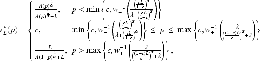
where
 is the agent’s loss-weighted odds ratio of event
 .
.
As before, the results are preserved under arbitrary positive linear rescaling of the payoffs. In other words, for any positive linear rescaling of the payoffs
 ,
,
 , the optimal consistent report remains
 and the corresponding optimal expected outcome is simply rescaled according to
 .
.
The decision maker should then calibrate the L-adjusted QSR by selecting the value of
 that solves
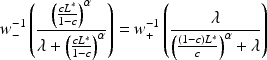
in order to eliminate the flat region of uninformative reports of
 .
.
Proofs of Propositions Footnote 1–Footnote 3 and Corollary Footnote 1
Proof of Proposition 1
This result is a special case of Proposition Footnote 3, with
 ,
,
 , and
, and
 . Note that directionality holds automatically if
 . To prove this, it is sufficient to show that
 for
for
 and
and
 for
for
 whenever the expectations
 and
and
 are both consistent. Observe that when
 ,
,
 where
where
 denotes a consistent expectation from reporting
 when the probability beliefs is
 . Since
 , we have that
 or
or
 . In particular, this means that
 and
and
 and
and
 are symmetric around
 . Then to prove directionality it suffices to show that
 is decreasing in
 . As shown in Proposition Footnote 3,
 .
.
 , where
 and
and
 , so
, so
 . Then by the chain rule
 , which implies that
 is decreasing in
 ,
,
 is increasing in
 , and the agent will prefer to report
 for
for
 and
and
 for
for
 .
.

Proof of Proposition 2
This result also follows from Proposition Footnote 3, by setting
 and comparing the case where
 , and
, and
 to the case of general
 and
and
 . The optimal consistent report function is the same in both cases, and after simplifying the expressions for the corresponding consistent expected outcome, we also have that
 for all
 .
.

Proof of Proposition 3
By Lemma 1 of Palley (Reference Palley2015), for any risky prospect that yields a payoff of
 with probability
 and
and
 with probability
 , where
 , there exists a unique consistent expected outcome
 such that
 , which means there will be a unique
 associated with any report
 Consider an L-adjusted asymmetric QSR whose payoffs have been rescaled by an arbitrary positive linear transformation
 ,
,
 . The agent must consider three separate cases when selecting the value of
 to report:

Case 1 (
 ):
):
 meaning that
 and
and
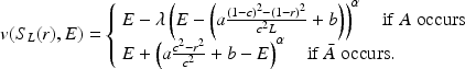
Consistency requires that
 so the consistent expectation for
 is
is
 , where

 is a concave quadratic function of
 , so its maximum occurs where
 meaning that
 However, this is only consistent for
 , so this reporting strategy is optimal only if
 , or equivalently, only if
 Then for all
 ,
,
 and for all
 , reporting
 is not optimal.
Case 2 (
 ):
):
 meaning that
 and
and

Consistency requires that
 so the consistent expectation for
 is
is

 is a concave quadratic function of
 , so its maximum occurs where
 meaning that
 However, this is only consistent for
 , so this reporting strategy is optimal only if
 , or equivalently, only if
 Then for all
 ,
,
 and for all
 , reporting
 is not optimal.
Case 3 (
 ):
):
 , meaning that
 and
and
 . Then consistency is satisfied since
 .
.
Then for any belief
 , the agent has three reporting choices:
1.
, in which case she will receive
2.
, in which case she will receive
, or3.
, in which case she will receive
.


If
 , then the only consistent report for
 is
is
 ,
,
 for
for
 , and
, and
 for
for
 .
.
If
 , then for
 we have
 , for
, for
 we have
 , and for
 we have
 . Under the assumption of directional reporting, this simply reduces to
 for
for
 and
and
 for
for
 .
.
The consistent ex ante expected outcome corresponding to the optimal consistent report
 is
is


Proof of Corollary 1
If
 , then we need
 to satisfy
 , or
, or
 . This means that
 , or
, or
 . Rearranging terms,
 which yields the desired result.


 c=0.5
c=0.5 A
A p=0.7
p=0.7 λ=2.4
λ=2.4 α=1
α=1

 r∗(p)
r∗(p) c=0.5
c=0.5 L=1
L=1 λ=2.4
λ=2.4 α=0.8
α=0.8 w-(p)=w+(p)=p
 rL∗(p)
 L=3.7
L=3.7 c=0.5
c=0.5 λ=2.4
λ=2.4 α=0.8
α=0.8 δ+=0.8
 γ+=0.7
 δ-=1.1
 γ-=0.7
 λ
λ α
α
 λ
λ
 r(p)
r(p) r=p
r=p

 r(p)
r(p) +/-
+/- r=p
r=p
 r(p)
r(p) r=p
r=p
 |r-p|
|r-p| r(p)
r(p)
 p
p r
r


 Open access