


1. Introduction
Buoyancy-driven convection is one of the key problems in a wide range of flows, including atmospheric convection (Hartmann, Moy & Fu Reference Hartmann, Moy and Fu2001), ocean convection (van Doorn et al. Reference van Doorn, Dhruva, Sreenivasan and Cassella2000) and geophysical convection (Glatzmaiers & Roberts Reference Glatzmaiers and Roberts1995). In buoyancy-driven convection, the flow obtains kinetic energy from its potential energy, which will spontaneously trigger and generate turbulence under certain conditions even without direct forcing, and the resulting flow exhibits complex phenomena due to the coupling of velocity and density. Owing to its simplicity in geometry and governing equation, Rayleigh–Bénard convection (RBC) is regarded as a canonical model representing buoyancy-driven convection for understanding, predicting and even controlling various scientific and application problems (Ahlers, Grossmann & Lohse Reference Ahlers, Grossmann and Lohse2009; Lohse & Xia Reference Lohse and Xia2010). In addition to the scalings of heat transfer and kinetic energy, which were successfully explained by Grossmann–Lohse (GL) theory (Grossmann & Lohse Reference Grossmann and Lohse2000, Reference Grossmann and Lohse2001, Reference Grossmann and Lohse2002; Ahlers et al. Reference Ahlers, Grossmann and Lohse2009; Lohse & Xia Reference Lohse and Xia2010), there are other fascinating flow behaviours in RBC, and large-scale circulation (LSC) and its reversal are among them (Benzi Reference Benzi2005; Brown & Ahlers Reference Brown and Ahlers2007, Reference Brown and Ahlers2008b; Assaf, Angheluta & Goldenfeld Reference Assaf, Angheluta and Goldenfeld2011; Petschel et al. Reference Petschel, Wilczek, Breuer, Friedrich and Hansen2011; Vasil'ev & Frick Reference Vasil'ev and Frick2011; Wagner & Shishkina Reference Wagner and Shishkina2013; Chen, Wang & Xi Reference Chen, Wang and Xi2020). In the past, flow reversals have been reported in cylindrical cells, two-dimensional (2-D) cavities as well as quasi-two-dimensional (quasi-2-D)/three-dimensional (3-D) cavities experimentally and numerically (Cioni, Ciliberto & Sommeria Reference Cioni, Ciliberto and Sommeria1997; Brown, Nikolaenko & Ahlers Reference Brown, Nikolaenko and Ahlers2005; Sun, Xi & Xia Reference Sun, Xi and Xia2005; Tsuji et al. Reference Tsuji, Mizuno, Mashiko and Sano2005; Xi & Xia Reference Xi and Xia2007, Reference Xi and Xia2008).
A comprehensive study was performed by Sugiyama et al. (Reference Sugiyama, Ni, Stevens, Chan, Zhou, Xi, Sun, Grossmann, Xia and Lohse2010), through both experiments and numerical simulations, to quantify the existence and frequency of flow reversals in 2-D and quasi-2-D geometry with a wide range of Rayleigh number  $Ra$ and Prandtl number
  $Pr$ (for definitions, see
  $\S$ 2.1). A phase diagram about the occurrence of flow reversals and the corresponding statistical results of reversal frequency were presented, together with a discussion on the dynamics of reversals. By introducing a Fourier decomposition, Chandra & Verma (Reference Chandra and Verma2011) studied the dynamics and symmetries of the flow reversals in 2-D RBC and observed that the amplitude of one of the large-scale modes almost vanishes while another mode rises sharply during the reversals. Chandra & Verma (Reference Chandra and Verma2013) further examined the mechanism of the flow reversals in 2-D RBC and argued that the vortex reconnection of two attracting corner rolls, which have the same sign of vorticity, will lead to major restructuring of the LSC and flow reversal. Castillo-Castellanos et al. (Reference Castillo-Castellanos, Sergent, Podvin and Rossi2019) identified two different types of flow regimes, i.e. consecutive flow reversals and extended cessations, for
  $Ra=10^6$ to
  $5\times 10^8$ and
  $Pr=3$ and 4.3, and used proper orthogonal decomposition and cluster-based analysis to investigate the flow modes in the two regimes. Besides analysis mainly based on simulations and experiments, there are some other works trying to capture the key mechanisms of reversals with stochastic (Sreenivasan, Bershadskii & Niemela Reference Sreenivasan, Bershadskii and Niemela2002) or deterministic (Araujo, Grossmann & Lohse Reference Araujo, Grossmann and Lohse2005) models in the form of ordinary differential equations. Other recent works presenting theoretical and numerical investigations on flow reversals include, but are not limited to, Ni, Huang & Xia (Reference Ni, Huang and Xia2015), Podvin & Sergent (Reference Podvin and Sergent2015), Chong et al. (Reference Chong, Wagner, Kaczorowski, Shishkina and Xia2018) and Chen et al. (Reference Chen, Huang, Xia and Xi2019).
In addition to the studies on RBC with classic set-ups, new flow set-ups are also introduced, including rough walls, varying fluid properties, and different velocity or temperature boundary conditions (Qiu, Xia & Tong Reference Qiu, Xia and Tong2005; Wang et al. Reference Wang, Xu, Xia, Wan and Sun2017; Zhang et al. Reference Zhang, Sun, Bao and Zhou2018; Zhu et al. Reference Zhu, Stevens, Shishkina, Verzicco and Lohse2019). These new set-ups may significantly influence flow structures, statistics and reversal behaviours. Huang et al. (Reference Huang, Wang, Xi and Xia2015) introduced the mixed boundary condition with one horizontal plate having fixed heat flux and they observed a decrease of reversal frequency as compared to the classic set-up with fixed temperature, suggesting that the reduction of symmetry may reduce the motivation of LSC to reverse. Xia et al. (Reference Xia, Wan, Liu, Wang and Sun2016) applied the low-Mach-number equation in the simulation of RBC to investigate the non-Oberbeck–Boussinesq effect and discovered different reversal properties. Wang et al. (Reference Wang, Xia, Wang, Sun, Zhou and Wan2018) investigated the flow reversals in 2-D cells with aspect ratio  $\varGamma =1$ (where
  $\varGamma =\textrm {width/height}$) and managed to efficiently suppress reversals by tilting the cavity. Chen et al. (Reference Chen, Wang and Xi2020) defined and identified reversals led by LSC and corner rolls separately, and reported that the total reversal frequency in a corner-less cell, where corner vortices are absent and the reversal is main-vortex-led, has the same piecewise scaling law and transition behaviour as that in a normal cell, where both main-vortex-led and corner-vortex-led reversals exist. Furthermore, they showed that the frequency of main-vortex-led reversals in a normal cell is in excellent agreement with that in a corner-less cell. Other interesting findings and analysis of the non-classic set-up can be found in Sun et al. (Reference Sun, Xi and Xia2005), Brown & Ahlers (Reference Brown and Ahlers2008a), Stevens, Lohse & Verzicco (Reference Stevens, Lohse and Verzicco2014), Wang et al. (Reference Wang, Xu, Xia, Wan and Sun2017), Wan et al. (Reference Wan, Wei, Verzicco, Lohse, Ahlers and Stevens2019) and Wang, Zhou & Sun (Reference Wang, Zhou and Sun2020).
Recently, Zhang et al. (Reference Zhang, Xia, Zhou and Chen2020) introduced a small constant-temperature region on both sidewalls in a 2-D square cavity. Direct numerical simulation results showed that effective suppression or activation of flow reversals can be realized with the proper location and size of the control regions. However, the work was limited to 2-D simulation results. In this paper, we extend the former work to quasi-2-D cases. In addition, a more symmetric control configuration with two control regions on each sidewall is also introduced, and the results are compared with the previous control configuration with one control region on each sidewall. The present paper is organized as follows. We first describe the basic equations along with numerical and experimental set-ups in § 2. The results and discussion related to the simulations at  $Ra=10^8$ and
  $Pr=2$ are presented in § 3. Experimental results and direct numerical results at higher
  $Ra$ are shown in § 4 in order to examine the realizability of control and further support the conclusions. Finally, § 5 will summarize the present work.
2. Basic set-ups
2.1. Governing equations and boundary conditions
In this paper, we consider turbulent RBC with Boussinesq approximation in 2-D and 3-D (quasi-2-D) geometry. The origin of the coordinates is defined at the centre of the cavity. For the 2-D cases, the cavity height  $\hat {H}$ (
 $y$ direction) and length
  $\hat {L}$ (
 $x$ direction) are the same, i.e. aspect ratio
  $\varGamma =\hat {L}/\hat {H}=1$; for the quasi-2-D cases, the width of the cavity is
  $\hat {W}=0.3\hat {H}$ (
 $z$ direction).
  $\hat {\boldsymbol {u}}=(\hat {u},\hat {v},\hat {w})$ is the velocity, with
  $\hat {u}$,
  $\hat {v}$ and
  $\hat {w}$ being the velocity components in the
  $x$,
$x$,  $y$ and
  $z$ (if it exists) directions, respectively;
  $\hat {\theta }$ is the temperature;
  $\hat {\theta }_{l}$ and
  $\hat {\theta }_u$ are the constant temperatures at the lower and upper walls, respectively;
  $\hat {\theta }_0=(\hat {\theta }_l+\hat {\theta }_u)/2$ is the bulk temperature; and
  ${\rm \Delta} \hat {\theta }=\hat {\theta }_{l}-\hat {\theta }_u$. The background temperature outside the sidewalls is set to
  $\hat {\theta }_0$. We define
  $\hat {\nu }$ as the kinematic viscosity,
  $\hat {\kappa }$ as the thermal diffusivity,
  $\hat {\lambda }$ as the thermal conductivity,
  $\hat {g}$ as the gravitational acceleration and
  $\hat {\beta }$ as the thermal expansion coefficient.
The free-fall velocity and the free-fall time can then be defined as  $\hat {U}=(\hat {g}\hat {\beta }{\rm \Delta} \hat {\theta }\hat {H})^{1/2}$ and
  $\hat {T}=\hat {H}/\hat {U}$, respectively. With velocity, time, length and temperature scales chosen as
  $\hat {U}$,
  $\hat {T}$,
  $\hat {H}$ and
  ${\rm \Delta} \hat {\theta }$, respectively, and with
  $\theta \triangleq (\hat {\theta }-\hat {\theta }_0)/{\rm \Delta} \hat {\theta }$, the governing equations and related boundary conditions can be non-dimensionalized as follows:
 \begin{equation} \left.\begin{array}{c@{}} \boldsymbol{\nabla} \boldsymbol{\cdot} \boldsymbol{u}=0,\\ \dfrac{\partial \boldsymbol{u}}{\partial t}+\boldsymbol{u}\boldsymbol{\cdot} \boldsymbol{\nabla} \boldsymbol{u}={-}\boldsymbol{\nabla} p+\dfrac{1}{\sqrt{Ra/Pr}}{\nabla^2\boldsymbol{u}}+\theta \boldsymbol{j},\\ \dfrac{\partial \theta }{\partial t}+\boldsymbol{u}\boldsymbol{\cdot} \boldsymbol{\nabla} \theta = \dfrac{1}{\sqrt{Ra\,Pr}}\nabla^2 \theta,\\ y={\pm} 0.5{:} \quad \boldsymbol{u}=0, \quad {\theta ={\mp} 0.5},\\ x={-}0.5{:}\quad \boldsymbol{u}=0, \quad {(\theta-\theta_0)-R_l{\partial\theta }/{\partial x}=0,}\\ x=0.5{:}\quad \boldsymbol{u}=0,\quad {(\theta-\theta_0)+R_r{\partial \theta}/{\partial x}=0,}\\ z={\pm} 0.15{:} \quad \boldsymbol{u}=0, \quad {\partial \theta }/{\partial z}=0 \quad{\text{(quasi-2-D)}}. \end{array}\right\}\end{equation}
 Here, the Rayleigh number is  $Ra={\hat {g}\hat {\beta }{\rm \Delta} \hat {\theta } \hat {H}^3}/{(\hat {\nu }\hat {\kappa })}$, the Prandtl number is
  $Pr= {\hat {\nu }}/{\hat {\kappa }}$, the normalized bulk temperature is
  $\theta _0=0$, and the normalized thermal resistances are
 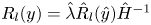 $R_l(y)=\hat {\lambda } \hat {R}_l(\hat {y})\hat {H}^{-1}$ and
  $R_r(y)=\hat {\lambda } \hat {R}_r(\hat {y})\hat {H}^{-1}$, where
  $\hat {R}_l(\hat {y})$ and
  $\hat {R}_r(\hat {y})$ are the thermal resistance per unit area at the left and right sidewalls, respectively. It is easy to see that
  $R_l(y)$ and
  $R_r(y)$ control the thermal boundary condition on the sidewalls. If
  $R_l(y)=R_r(y)=\infty$, the above governing equations correspond to the classic set-up with adiabatic left and right sidewalls, i.e.
  ${\partial \theta }/{\partial x}=0$ on the left and right sidewalls. Furthermore,
  $R_l(y_0)=0$ can lead to a local isothermal boundary condition with
  $\theta =\theta _0$. Zhang et al. (Reference Zhang, Xia, Zhou and Chen2020) introduced a local
  $R_l(y)=0$ region on the left sidewall and a local
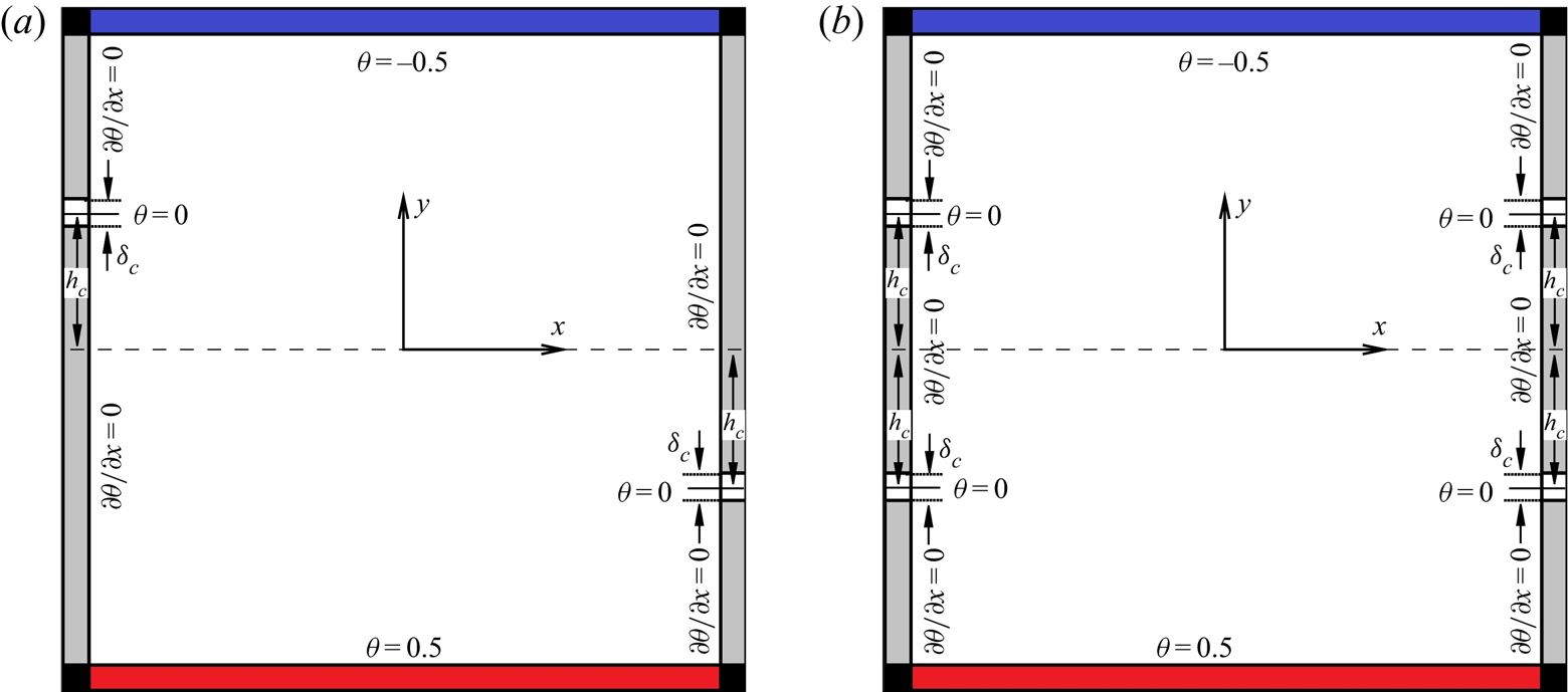
  $R_r(y)=0$ region on the right sidewall, as shown in figure 1(a), and the coefficients governing the temperature conditions on the sidewalls are
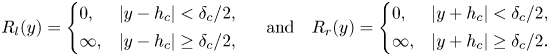 \begin{equation} R_l(y)= \left\{ \begin{array}{@{}ll} 0, & |y-h_c|<\delta_c/2,\\ \infty, & |y-h_c|\geq \delta_c/2, \end{array} \right.\quad \mathrm{and}\quad R_r(y)= \left\{ \begin{array}{@{}ll} 0, & |y+h_c|<\delta_c/2,\\ \infty, & |y+h_c|\geq \delta_c/2. \end{array} \right.\end{equation}
We denote the configuration with coefficients (2.2a,b) as the two-point control configuration. It should be noted that the formulations of the boundary condition on the left and right sidewalls are different from those used in Zhang et al. (Reference Zhang, Xia, Zhou and Chen2020), where they used two control parameters to simply combine the isothermal and adiabatic boundary conditions together. Here, we introduce the thermal resistance and the formulae for the boundary conditions are of clear physical meaning.

Figure 1. Sketches of sidewall controlled 2-D RBC with  $h_c>0$: (a) two-point control and (b) four-point control. In quasi-2-D RBC, the
  $z$ direction points out from the paper and adiabatic conditions are applied on both sidewalls in the
  $z$ direction.
In addition, a new configuration with two control regions on each (left/right) sidewall is introduced and  $R_l$ and
  $R_r$ are defined as
 \begin{equation} R_l(y)=R_r(y)= \left\{ \begin{array}{@{}ll} 0, & ||y|-h_c|<\delta_c/2,\\ \infty, & ||y|-h_c|\geq \delta_c/2. \end{array} \right.\end{equation}
This new symmetric configuration is shown in figure 1(b) and it is denoted as the four-point control configuration. It is seen that, with  $h_c=0$, the two-point control and the four-point control are the same.
2.2. Numerical set-up
For both 2-D and quasi-2-D simulations, the second-order finite difference code AFiD (Van Der Poel et al. Reference Van Der Poel, Ostilla-Mónico, Donners and Verzicco2015) is used with some modifications, where the discretized Poisson equation is decoupled using a discrete cosine transform in horizontal directions and solved with a tridiagonal solver, while the time marching is realized with the second-order explicit Adams–Bashforth scheme. Figure 2 shows the time-averaged Nusselt number  $\langle Nu\rangle _t$ (see the definition below) obtained using the present code with different numbers of grid points in a cubic RBC cell at
  $Ra=1\times 10^8$ and
  $Pr=1$. The results shown in Kooij et al. (Reference Kooij, Botchev, Frederix, Geurts, Horn, Lohse, van der Poel, Shishkina, Stevens and Verzicco2018) from another validated code GOLDFISH are also included as reference. It is seen that the
  $\langle Nu\rangle _t$ computed with the present code could converge to an accurate value with increasing number of grid points, indicating the correctness of the present code.
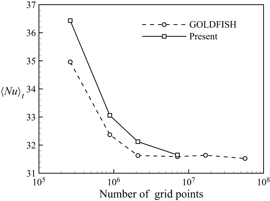
Figure 2. Plot of  $\langle Nu\rangle _t$ in a cubic RBC cell at
  $Ra=1\times 10^8$ and
  $Pr=1$ obtained using the present code with different numbers of grid points. The results reported in Kooij et al. (Reference Kooij, Botchev, Frederix, Geurts, Horn, Lohse, van der Poel, Shishkina, Stevens and Verzicco2018) from the validated code GOLDFISH are also shown for comparison.
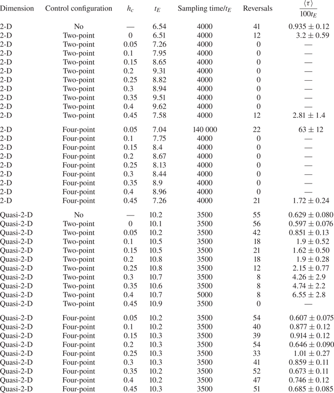
In this paper, the widths of the control regions are kept the same and they are fixed as  $\delta _c=0.05$. We mainly focus on the cases at
  $Ra=10^8$ and
  $Pr=2$, where both 2-D and quasi-2-D simulations are performed with the two-point control configuration, the four-point control configuration, as well as the classic adiabatic configuration (no control). For the two-point control configuration,
  $h_c$ varies in
  $[0,0.45]$ with an increment of
  $0.05$, while for the four-point control configuration
  $h_c$ varies in
  $[0.05,0.45]$ with the same increment of
  $0.05$. For comparison with the experimental results, we perform quasi-2-D simulations at
  $Ra=1.93\times 10^8$ and
  $Pr=5.7$ with two-point
  $h_c\in \{0,0.15\}$ control and without control, and also at
  $Ra=7.36\times 10^8$ and
  $Pr=5.7$ with
  $h_c=0$ control and without control. The parameters of the simulations are listed in table 1.
Table 1. Parameters of the 2-D and quasi-2-D simulations with  $Ra=10^8$ and
  $Pr=2$.

For the 2-D simulations, the grid size is  $192\times 192$. For the quasi-2-D simulations, the mesh is
  $192\times 192\times 64$ at
  $Ra=10^8$ and
  $Ra=1.93\times 10^8$ and it is
  $256\times 256\times 72$ at
  $Ra=7.36\times 10^8$. For all the simulation cases, the mesh is uniform in the horizontal directions (
 $x$ and
  $z$ directions) while it is refined near the walls in the vertical direction (
 $y$ direction) to make sure that the grid size
  $\hat {\varDelta }$ satisfies
  $\hat {\varDelta }<0.6\min [\widehat {\eta _K},\widehat {\eta _B}]$ in the boundary layers. The numbers of grid points in the
  $x$ and
  $y$ directions for the
  $Ra=10^8$ simulations are the same as in the present validation case with the largest grid size. Here
  $\widehat {\eta _K}= [\hat {\nu }^3/\hat {\varepsilon }(\hat {\boldsymbol {x}},\hat {t})]^{1/4}/\hat {H}$ (with
  $\hat {\varepsilon }(\hat {\boldsymbol {x}},\hat {t})$ being the local turbulent dissipation) is the local Kolmogorov scale and
  $\widehat {\eta _B}=\widehat {\eta _K} Pr^{-1/2}$ is the Batchelor scale. The time steps are small enough to make sure that the Courant–Friedrichs–Lewy numbers are smaller than
  $0.2$.
For convenience in expression, any 2-D field  $\phi (x,y,t)$ could be rewritten as
  $\phi (x,y,z,t)$ with the extra dimension being trivial with
  $\partial \phi /\partial z \equiv 0$, and we could also define
  $w\equiv 0$. In the following,
  $\langle \cdot \rangle _t$,
  $\langle \cdot \rangle _x$,
  $\langle \cdot \rangle _y$ and
  $\langle \cdot \rangle _z$ denote the averages in time, along the
  $x$ axis, along the
  $y$ axis and along the
  $z$ axis, respectively; and
  $\langle \cdot \rangle _V$ denotes the volume average. Following the definition in Sugiyama et al. (Reference Sugiyama, Ni, Stevens, Chan, Zhou, Xi, Sun, Grossmann, Xia and Lohse2010), the LSC turnover time
  $t_E$ in both 2-D and quasi-2-D simulation cases is defined as
  $t_E=4{\rm \pi} /\langle |\omega _z(0,0,0,t)|\rangle _t$, where
  $\omega _z(0,0,0,t)$ is the central vorticity in the
  $z$ direction. The reversal indicator is defined as the volume-averaged angular momentum
 \begin{equation} L( t )={{\langle x v-y u \rangle }_V}.\end{equation}
The value  $L<0$ usually corresponds to a clockwise LSC and vice versa, which is the same as in Zhang et al. (Reference Zhang, Xia, Zhou and Chen2020). All simulations are run for more than
  $2500t_E$ in order to obtain reasonable estimations on the reversal interval and flow statistics.
2.3. Experimental set-up
We also perform experiments to measure of the LSC at higher  $Ra$ for the two-point control configuration. The experimental set-up used here is almost the same as that in Chen et al. (Reference Chen, Huang, Xia and Xi2019), with the size of the fluid region being
  $\hat {H}=\hat {L}=12.6$ cm and
  $\hat {W}=3.8~\textrm {cm}\approx 0.3\hat {H}$. The fluid is bounded with vertical walls mainly made of Plexiglas and horizontal plates made of copper. A refrigerated circulator (PolyScience) and two resistive film heaters are used to maintain isothermal boundary conditions at the top and bottom plates, respectively. A locally isothermal boundary condition on the sidewalls is realized with inserted copper blocks (of size
  $\delta _c=0.05\hat {H}$) conducting heat between the air and the working fluid, while the fluid–solid interface is kept flat. During the experiment, the convection cell is put in a thermostatic box with its interior temperature regulated at
  $28\,^{\circ }$C. Deionized water is chosen as the working fluid. As a result, the
  $Pr$ of the working fluid is
  $5.7$. Six thermistors are embedded in the bottom plate at approximately
  ${8}$ mm below the fluid–solid interface, with horizontal coordinates
  $\hat {x}=0$,
  $\pm \hat {L}/4$ and
  $\hat {z}=\pm {5}$ mm, respectively. The temperature obtained from the two thermistors on the left (
 $\hat {x}=-\hat {L}/4,\ \hat {z}=\pm {5}$ mm) are denoted as
  $\hat {\theta }_{left}$, and the temperature obtained from the two thermistors on the right (
 $\hat {x}=\hat {L}/4,\ \hat {z}=\pm {5}$ mm) are denoted as
  $\hat {\theta }_{right}$. There are another six thermistors embedded in the top plate with the same configuration. In order to test the capability of the copper blocks to realize the isothermal boundary condition, a thermistor is embedded in the centre of a copper block in a test case with
  $Ra=1.93\times 10^8$ and two-point
  $h_c=0.15$ control. The temperature of the copper block fluctuates with a mean of
  $28.32\,^{\circ }$C and a root-mean-square (r.m.s.) value of
  $1.35\times 10^{-2\,\circ }$C, indicating that copper blocks can achieve a local isothermal boundary condition with bulk temperature approximately.
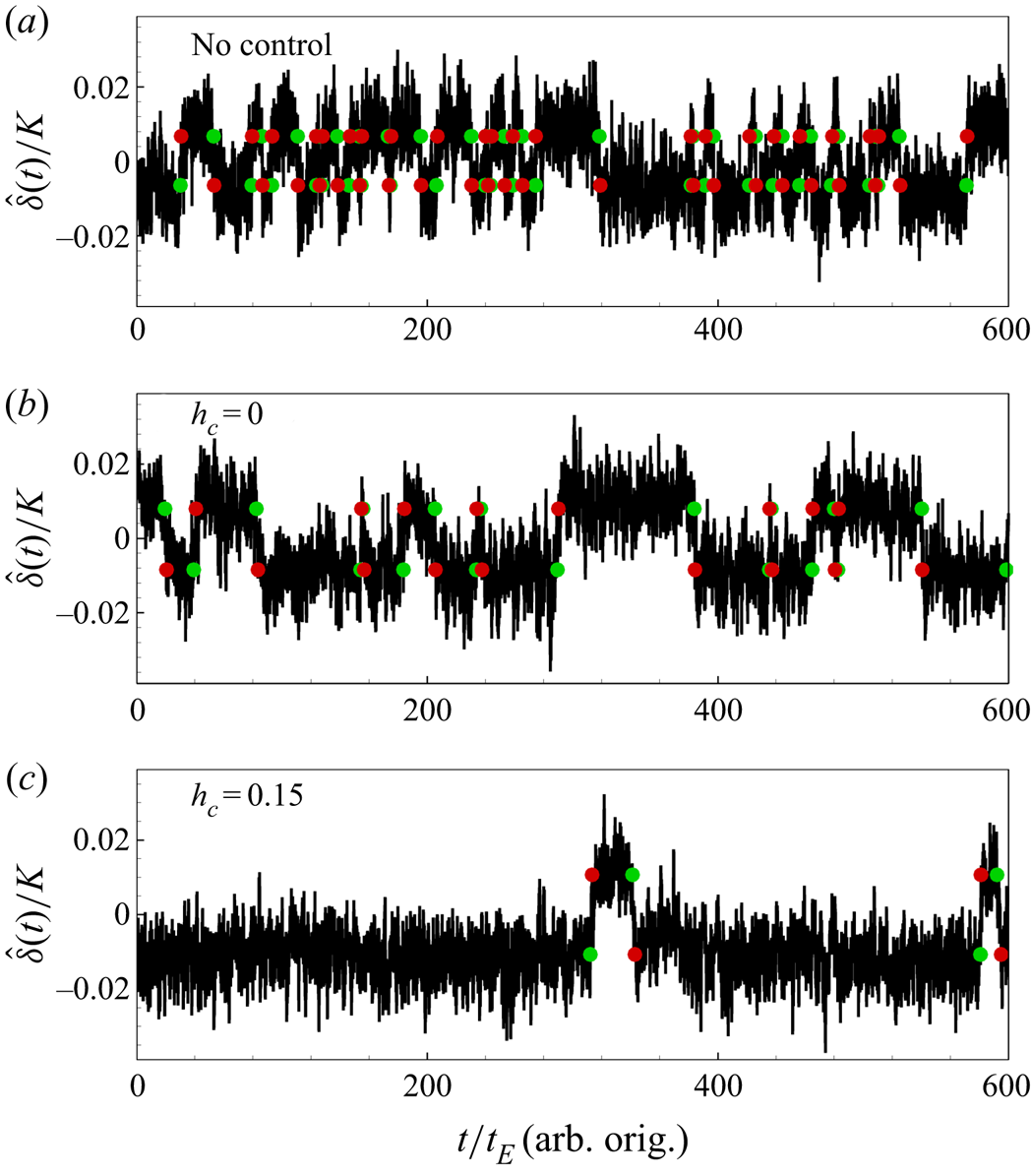
In the experiments,  $h_c$ is chosen to be 0 and 0.15. For
  $h_c=0$, measurements are performed with
  $Ra=1.92\times 10^8,\ 2.71\times 10^8,\ 5.56\times 10^8$ and
  $7.36\times 10^8$. For
  $h_c=0.15$, measurements are carried out with
  $Ra=1.37\times 10^8,\ 1.93\times 10^8$ and
  $2.71\times 10^8$. The parameters of the experiments are given in table 2. For the experimental cases, the LSC turnover time is obtained by the cross-correlation of the measured temperature signals inside the bottom plates following Brown, Funfschilling & Ahlers (Reference Brown, Funfschilling and Ahlers2007). All measurements are performed for over
  $1500t_E$ for estimation of reversal intervals and statistics. Here,
  $t_E$ is estimated based on the cross-correlation of the temperature signals inside the plates, and data for the no-control experimental cases are obtained from the previous experiments described in Chen et al. (Reference Chen, Huang, Xia and Xi2019). The reversal indicator (or flow strength) is chosen as the temperature difference measured between the right and left thermistors in the bottom plate:
 \begin{equation} \hat{\delta}( t )=\hat{\theta}_{right}-\hat{\theta}_{left}.\end{equation}
A value  $\hat {\delta }<0$ usually corresponds to a clockwise LSC and vice versa, which is in accordance with Chen et al. (Reference Chen, Huang, Xia and Xi2019).
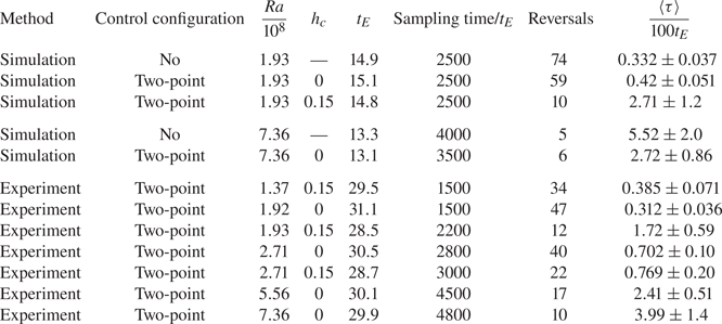
Table 2. Parameters of simulations and experiments with  $Ra>10^8$ and
  $Pr=5.7$. The
  $t_E$ value is estimated differently in simulations and experiments.
2.4. Reversal detection
In this section,  $\xi (t)$ is used to represent the generic reversal indicator, which represents
  $L(t)$ in simulations and
  $\hat {\delta }(t)$ in the experiments, for simplicity. In order to identify the reversal events with the time series of
  $\xi (t)$, the criterion of reversals proposed by Huang & Xia (Reference Huang and Xia2016) is adapted here with small changes. According to Huang & Xia (Reference Huang and Xia2016), the probability density function (p.d.f.) of
  $\xi$ for traditional no-control cases should have two distinct peaks, and a double-Gaussian fit could be applied to identify the locations of the two peaks as
  $\xi ^{(-)}$ and
  $\xi ^{(+)}$, which are then defined as thresholds for the starting or ending of reversals. However, with proper set-ups in two-point control configuration, the system may strongly prefer a clockwise LSC over an anticlockwise one, resulting in a decreasing height of the peak in
  $\xi >0$. Generally, if the peak in
  $\xi >0$ can still be discerned, then the locations of the peaks can be chosen as
  $\xi ^{(-)}$ and
  $\xi ^{(+)}$, respectively. In some cases, when the peak in
  $\xi >0$ disappears,
  $\xi ^{(+)}$ should be chosen as
  $-\xi ^{(-)}$, with
  $\xi ^{(-)}$ being the location of the peak in
  $\xi <0$. The rest of the criterion is the same as introduced in Huang & Xia (Reference Huang and Xia2016). For example, if the LSC reverses from anticlockwise state to clockwise state,
  $\xi (t)$ should shift from
  $\xi <\xi ^{(-)}$ to
  $\xi >\xi ^{(+)}$ and remain larger than
  $\xi ^{(-)}$ for at least
  $t_E$ before reversing back.
When the reversal criterion is defined, we can then quantitatively characterize the flow reversal. Following Sugiyama et al. (Reference Sugiyama, Ni, Stevens, Chan, Zhou, Xi, Sun, Grossmann, Xia and Lohse2010),  $\tau$ is used to denote the time interval between two successive reversals, and
  $\langle \tau \rangle$, the mean time interval between successive reversals, can represent the reversal feature for a general RBC system where it does not prefer any LSC orientation. However, as mentioned above and verified in Zhang et al. (Reference Zhang, Xia, Zhou and Chen2020) and below, the controlled system with the symmetry-broken two-point control configuration (
 $h_c>0$) may prefer certain LSC orientation, and thus the reversal activity could be characterized more delicately. We use
  $\tau _-$ to denote the time interval between an ‘anticlockwise to clockwise’ reversal and a successive ‘clockwise to anticlockwise’ reversal. Accordingly,
  $\tau _+$ denotes the time interval between a ‘clockwise to anticlockwise’ reversal and a successive ‘anticlockwise to clockwise’ reversal. In other words,
  $\tau _-$ and
  $\tau _+$ are the time span of the system when it is in the clockwise state and anticlockwise state, respectively, between two successive reversals;
  $N_-$ and
  $N_+$ denote the numbers of detected
  $\tau _-$ and
  $\tau _+$ respectively; and
  $\langle \tau _-\rangle$ and
  $\langle \tau _+\rangle$ denote the average of detected
  $\tau _-$ and
  $\tau _+$, respectively. Thus, one can write
 \begin{equation} \langle\tau_-\rangle=\frac{1}{N_-}\sum_{i=1}^{N_-}\tau_{-,i},\quad \langle\tau_+\rangle=\frac{1}{N_+}\sum_{i=1}^{N_+}\tau_{+,i}. \end{equation}
The error bars of  $\langle \tau _-\rangle$ and
  $\langle \tau _+\rangle$ are the standard deviations
  $\sqrt {\langle (\tau _--\langle \tau _-\rangle )^2\rangle /N_-}$ and
  $\sqrt {\langle (\tau _+-\langle \tau _+\rangle )^2\rangle /N_+}$, respectively. The mean value of the two kinds of time intervals is defined as
  $\langle \tau \rangle \triangleq (\langle \tau _-\rangle +\langle \tau _+\rangle )/2$ with error bar quantified using
  $\sqrt {\langle (\tau _--\langle \tau _-\rangle )^2\rangle /N_- +\langle (\tau _+-\langle \tau _+\rangle )^2\rangle /N_+}/2$. It should be noted that, when the system does not prefer any LSC orientation,
  $N_-\approx N_+$ and
  $\langle \tau _-\rangle \approx \langle \tau _+\rangle$, the above definitions of
  $\langle \tau \rangle$ and its error bar will be degenerated to their traditional definitions.
3. Numerical results at  $Ra=10^8$ and $Pr=2$


3.1. Suppression/activation of reversals
In the previous work, Zhang et al. (Reference Zhang, Xia, Zhou and Chen2020) showed that two-point control with different  $h_c$ and
  $\delta _c$ can either suppress or enhance the flow reversals in a 2-D cavity at different
  $Ra$ and
  $Pr$. In this subsection, we will focus on the influences of the two-point and four-point control configurations on the flow reversals in 2-D and quasi-2-D cavities at
  $Ra=10^8$ and
  $Pr=2$ when
  $\delta _c=0.05$ is fixed.
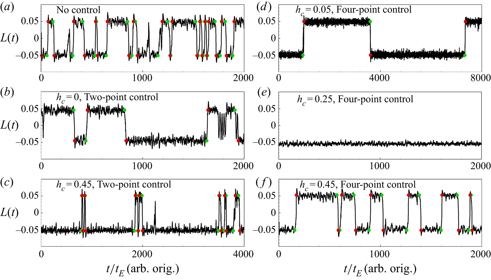
Figure 3 shows the time series of  $L(t)$ from six different 2-D simulations at
  $Ra=10^8$ and
  $Pr=2$. When there is no control on the sidewalls, flow reversals happen frequently and randomly, as shown in figure 3(a). The system does not prefer a certain LSC orientation, and
  $\langle \tau \rangle _0\approx \langle \tau _-\rangle \approx \langle \tau _+\rangle =93.5\pm 12 t_E$. We take this
  $\langle \tau \rangle _0$ as a reference. When the two-point control is applied at the centre of the sidewalls, i.e.
  $h_c=0$, as displayed in figure 3(b), flow reversals can still be observed. However, the number of reversal events reduces very obviously as compared to the no-control case. Although the system still does not favour a certain LSC orientation due to the fact that the control is symmetric, it can stay in a certain state for much longer time, resulting in much larger
  $\langle \tau \rangle$. Nevertheless, when the location of the two-point control moves away from the centre, the symmetry of the system is broken and it prefers the clockwise state with
  $h_c>0$. When
  $0.05\leq h_c\leq 0.4$, the flow reversal is entirely eliminated, as listed in table 1. For an extreme case with
  $h_c=0.45$, as depicted in figure 3(c), although flow reversals still happen, the system will reverse back very soon and stay in the clockwise state for most of the time. In this case,
  $\langle \tau _-\rangle$ is much larger than
  $\langle \tau \rangle _0$ while
  $\langle \tau _+\rangle$ is much smaller than
  $\langle \tau \rangle _0$, but the overall mean value of the time intervals
  $\langle \tau \rangle$ is still larger than
  $\langle \tau \rangle _0$, indicating that the sidewall control can still suppress the flow reversal. For the symmetric four-point control configuration, the sidewall control can still suppress the flow reversal (see the values of
  $\langle \tau \rangle$ in table 1), and the flow reversal events occur much less frequently, as shown in figure 3(d) with
  $h_c=0.05$ and in figure 3(f) with
  $h_c=0.45$, and no reversal can be observed for
  $h_c=0.25$, as shown in figure 3(e).

Figure 3. Time series  $L(t)$ of 2-D simulations at
  $Ra=10^8$ and
  $Pr=2$: (a) no control; (b) two-point control with
  $h_c=0$; (c) two-point control with
  $h_c=0.45$; (d) four-point control with
  $h_c=0.05$; (e) four-point control with
  $h_c=0.25$; and (f) four-point control with
  $h_c=0.45$. The origins of time are chosen differently for each case (arb. orig.). Green and red circles represent reversal starts and ends, respectively.
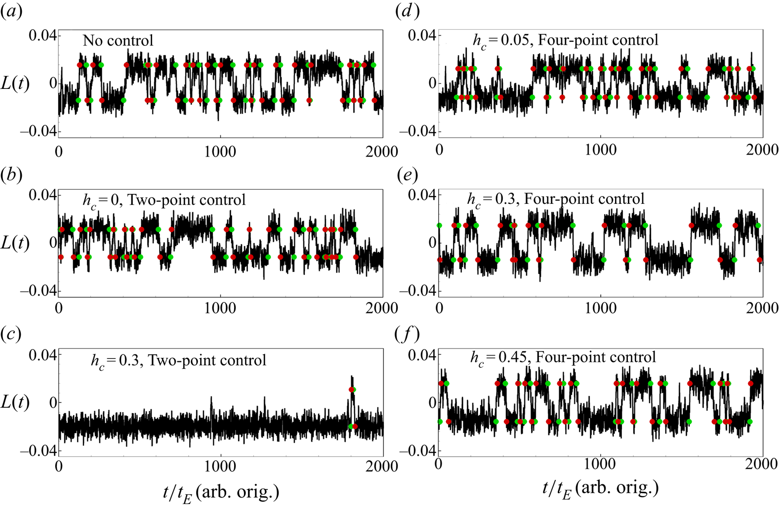
Figure 4 shows the time series of  $L(t)$ from six different quasi-2-D simulations at
  $Ra=10^8$ and
  $Pr=2$. For the no-control case shown in figure 4(a), we can observe the frequently and randomly occurring flow reversals, and
  $\langle \tau \rangle _0\approx 62.9\pm 8.0t_E$. Different from the 2-D results, the two-point control with
  $h_c=0$ has little effect on controlling the flow reversals,
  $\langle \tau \rangle \approx 59.7\pm 7.6t_E$, and no clear conclusion can be made from figure 4(b). When
  $h_c$ increases,
  $\langle \tau \rangle$ increases and the system favours the clockwise LSC. For
  $h_c=0.3$ as shown in figure 4(c), we can only observe two flow reversals for a time span
  $2000t_E$ and the system is at the clockwise LSC state for more than
  $1950t_E$. When
  $h_c$ further increases to 0.45, the flow reversals are fully suppressed, as listed in table 1. For the four-point control configuration, the control effect is much weaker. For
  $h_c=0.05$ shown in figure 4(d) (
 $\langle \tau \rangle \approx 60.7\pm 7.5t_E$) and
  $h_c=0.45$ shown in figure 4(f) (
 $\langle \tau \rangle \approx 68.5\pm 8.5t_E$), no clear difference in the reversal events can be observed as compared to the no-control case shown in figure 4(a) (
 $\langle \tau \rangle _0\approx 62.9\pm 8.0t_E$). For
  $h_c=0.3$ shown in figure 4(e) (
 $\langle \tau \rangle \approx 85.9\pm 11.0t_E$), the number of reversal events becomes much less and the flow reversals are suppressed.

Figure 4. Time series  $L(t)$ of quasi-2-D simulations at
  $Ra=10^8$ and
  $Pr=2$: (a) no control; (b) two-point control with
  $h_c=0$; (c) two-point control with
  $h_c=0.3$; (d) four-point control with
  $h_c=0.05$; (e) four-point control with
  $h_c=0.3$; and (f) four-point control with
  $h_c=0.45$. The origins of time are chosen differently for each case (arb. orig.). Green and red circles represent reversal starts and ends, respectively.
In order to characterize the control effect quantitatively, we plot in figure 5  $\langle \tau _-\rangle /\langle \tau \rangle _0$ and
  $\langle \tau _+\rangle /\langle \tau \rangle _0$ for the two-point control and
  $\langle \tau \rangle /\langle \tau \rangle _0$ for the four-point control from the 2-D and quasi-2-D simulations at
  $Ra=10^8$ and
  $Pr=2$ with different
  $h_c$. Here,
  $\langle \tau \rangle _0$ is the mean time interval between successive reversals from the no-control case. As discussed above, due to the symmetry-breaking property of the two-point control configuration, the system will prefer a certain LSC orientation, and thus
  $\langle \tau _-\rangle$ and
  $\langle \tau _+\rangle$ will be different and they are obtained separately. The overall
 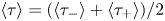 $\langle \tau \rangle =(\langle \tau _-\rangle +\langle \tau _+\rangle )/2$ at different
  $h_c$ are listed in table 1 and will not be shown here. If the reversals are fully eliminated,
  $\langle \tau \rangle$ would be infinity and they will not be shown with symbols in figure 5.
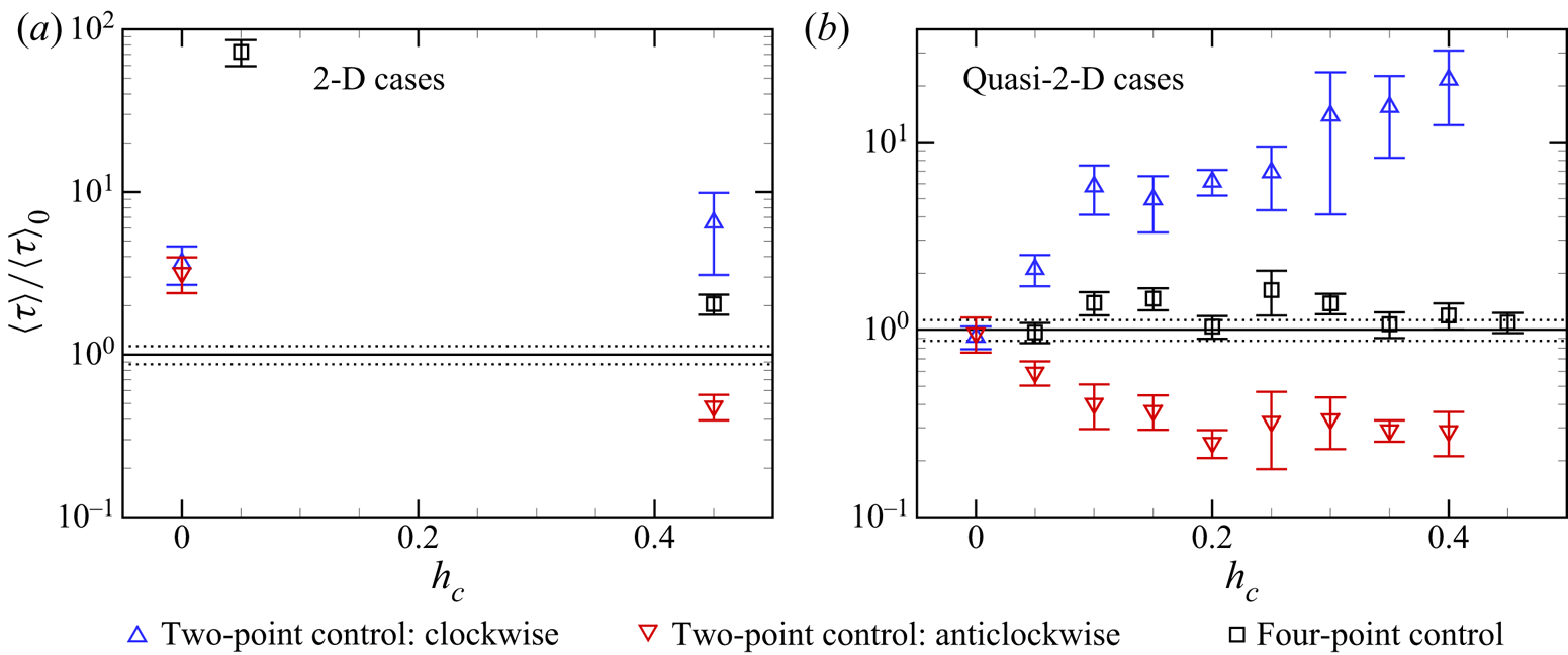
Figure 5. Plots of  $\langle \tau _-\rangle /\langle \tau \rangle _0$ and
  $\langle \tau _+\rangle /\langle \tau \rangle _0$ for the two-point control and
  $\langle \tau \rangle /\langle \tau \rangle _0$ for the four-point control from the (a) 2-D and (b) quasi-2-D simulations at
  $Ra=10^8$ and
  $Pr=2$ with
  $0\leq h_c\leq 0.45$. Here
  $\langle \tau \rangle _0$ is the mean time interval between successive reversals from the no-control case. Dotted lines represent the error bars of
  $\langle \tau \rangle _0$. Symbols
  $\triangle$ and
  $\triangledown$ denote
  $\langle \tau _-\rangle$ and
  $\langle \tau _+\rangle$ in the two-point control configuration, respectively. If the reversals are fully eliminated at certain
  $h_c$, there will be no symbol shown.
For the 2-D cavity shown in figure 5(a), it is evident that both the two-point and four-point controls can suppress the flow reversal effectively for  $0\leq h_c\leq 0.45$. For the two-point control configuration, the sidewall control can fully eliminate the flow reversal when
  $0.05\leq h_c\leq 0.4$, and it will make the system favour the clockwise LSC orientation when
  $h_c=0.45$. For the four-point control, the control can also fully eliminate the flow reversal when
 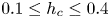 $0.1\leq h_c\leq 0.4$, and it can result in a stronger reversal suppression for
  $h_c=0.05$ than for
  $h_c=0.45$. For the quasi-2-D cavity shown in figure 5(b), the sidewall control may not be so effective as those in a 2-D cavity for both configurations. The two-point control with
  $h_c>0$ can suppress the flow reversals again and the system favours the clockwise LSC orientation since
 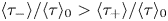 $\langle \tau _-\rangle /\langle \tau \rangle _0>\langle \tau _+\rangle /\langle \tau \rangle _0$. The value of
  $\langle \tau _-\rangle /\langle \tau \rangle _0$ generally increases with
  $h_c$ and the reversals are fully suppressed when
  $h_c=0.45$, indicating that the two-point control is more effective in suppressing the flow reversal when
  $h_c$ is larger. For the four-point control, it can generally suppress the flow reversal very mildly when
  $0.1\leq h_c\leq 0.45$, but the suppression effect is not monotonic with
  $h_c$ as is the two-point control and the efficiency is relatively lower. With
  $h_c=0.1,\ 0.15,\ 0.25$ and
  $0.3$, the control can suppress the flow reversal considerably.
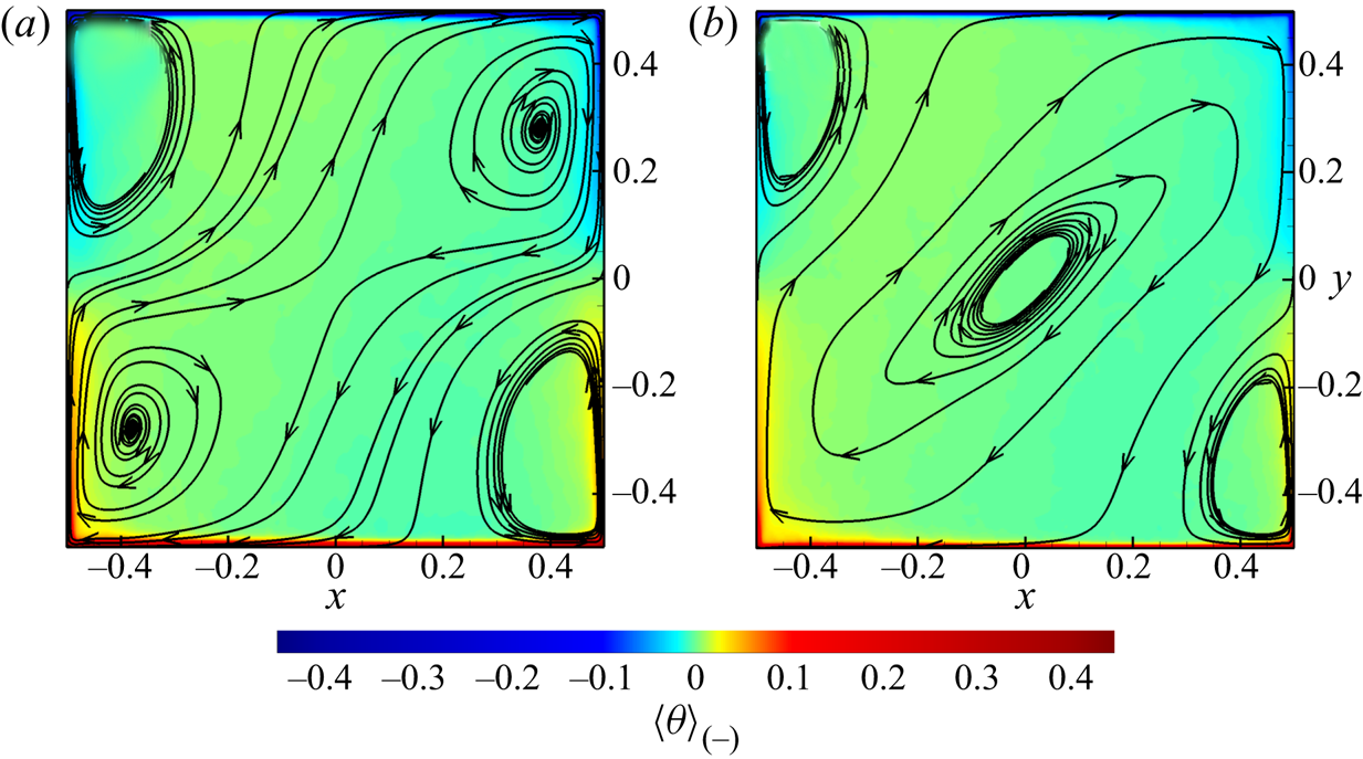
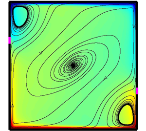
Figure 6 shows the temperature contours, the in-plane velocity vectors and the in-plane  $\boldsymbol {F}^b$ vectors
  $(F_x^b, F_y^b)$ from instantaneous flow fields with the two-point control and four-point control configurations in 2-D and quasi-2-D cavities. Here,
 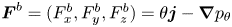 $\boldsymbol {F}^b=(F_x^b, F_y^b, F_z^b)=\theta \boldsymbol {j}-\boldsymbol {\nabla } p_{\theta }$ is the divergence-free projection of the buoyancy force, with
  $p_{\theta }$ being the pressure required to eliminate the divergence of the buoyancy force (Zhang et al. Reference Zhang, Xia, Zhou and Chen2020):
 \begin{align} \nabla^2 p_\theta={\partial \theta}/{\partial y},\quad {\partial p_\theta}/{\partial x}|_{x=\pm0.5}={\partial p_\theta}/{\partial z}|_{z=\pm0.15}=0,\quad {\partial p_\theta}/{\partial y}|_{y=\pm0.5}=\theta. \end{align}
From the momentum equation, it can be inferred that  $\boldsymbol {F}^b$ is the only source for the control region to instantly influence the evolution of the velocity field. As shown in figure 6(a3,b3,c3,d3), the hot plume with
  $\theta >0$ rising along the right sidewall may contact with the local zone with
  $\theta \approx 0$ and result in a local
  $\partial \theta /\partial y<0$ zone close to the control area. The negative
  $\partial \theta /\partial y$ appears as the source term in (3.1a–c), which contributes positively to
  $\partial p_{\theta }/\partial x$ and thus negatively to
  $F^b_x$ on the left side of this
  $\partial \theta /\partial y<0$ region, according to the Green's function. Similarly, when a cold plume descending along the right sidewall meets with the control region (see figure 6b2,d2), there would also be a local region contributing negatively to
  $F^b_x$. In other words, when a descending cold plume or rising hot plume meets with the control region on a sidewall, the resulting negative
  $\partial \theta /\partial y$ tends to force
  $\boldsymbol {F}^b$ to point away from the corresponding sidewall. Therefore, the control region tends to drive any plume it touches to separate, and thus weakens or restrains the corresponding vortex (LSC or corner rolls) fed by the plume. Another effect of control regions on the vortices is to reduce the
  $|\theta |$ of plumes through thermal conduction, and consequently to reduce the
  $v\theta$, which is the production term of kinetic energy.

Figure 6. Temperature contours (colour), in-plane velocity vectors (black) and in-plane  $\boldsymbol {F}^b$ vectors (white) of instantaneous fields in the
  $z=0$ plane. The lengths of the vectors are proportional to their magnitudes. The control parameters are
  $Ra=10^8$ and
  $Pr=2$. Panels: (a1,a2,a3) 2-D and two-point control,
  $h_c=0.25,\ t_E=2.5\times 10^3$; (b1,b2,b3) 2-D and four-point control,
  $h_c=0.25,\ t_E=3.5\times 10^3$; (c1,c2,c3) quasi-2-D and two-point control,
  $h_c=0.3,\ t_E=3.5\times 10^3$; (d1,d2,d3) quasi-2-D and four-point control,
  $h_c=0.3,\ t_E=0.7\times 10^3$. Panels (a1,b1,c1,d1) show the temperature contours and in-plane velocity vectors in the whole domain; (a2,b2,c2,d2) show the zoomed-in temperature contours, in-plane velocity vectors (black) and in-plane
  $\boldsymbol {F}^b$ vectors (white) near the upper-right control region (if it exists); (a3,b3,c3,d3) show the zoomed-in temperature contours, in-plane velocity vectors (black) and in-plane
  $\boldsymbol {F}^b$ vectors (white) near the lower-right control region.
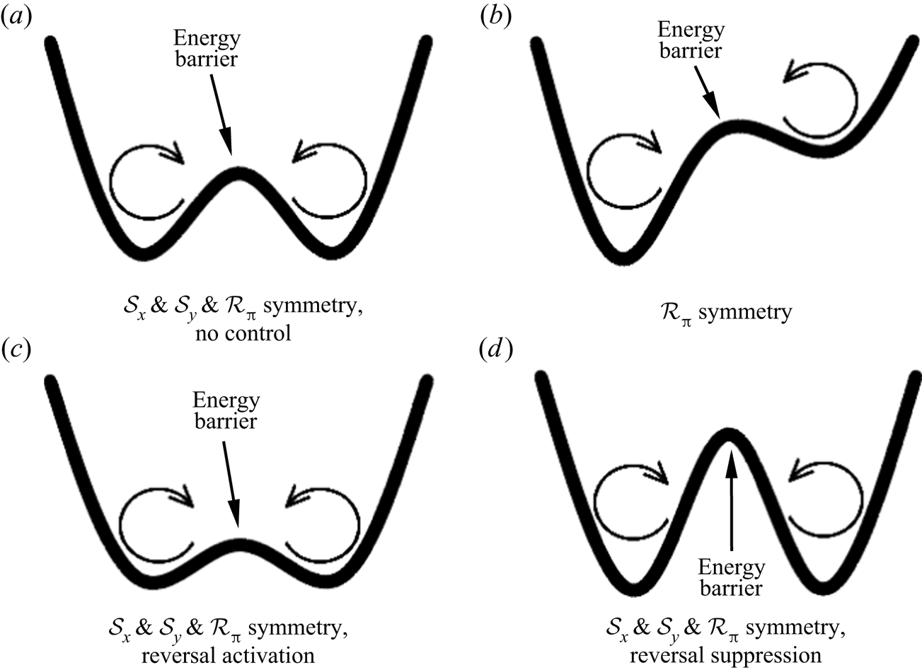
In all, the control region has two approaches to restrain or weaken a vortex that it contacts with, either through the instant  $\boldsymbol {F}^b$ or through the slow thermal conduction. Specifically, if a control region contacts with the LSC, it will weaken the LSC and implicitly provide more opportunity for the growth of corner rolls, motivating the LSC to reverse. If the control region contacts with a corner roll, it will suppress the growth of the corner roll and implicitly strengthen the LSC, which helps to stabilize the LSC. For a clockwise state and
  $h_c>0$, the two control regions in the second and fourth quadrants from both control configurations would weaken the corner roll when they grow large enough, but the two extra control regions in the first and third quadrants from the four-point control would weaken the LSC. Therefore, the clockwise LSC is less stable under the four-point control as compared to the two-point control. For an anticlockwise state and
  $h_c>0$, the two control regions in the second and fourth quadrants from both control configurations would weaken the LSC, but the two extra control regions in the first and third quadrants from the four-point control would weaken the corner rolls when they grow large enough. Therefore, the anticlockwise LSC is more stable under the four-point control as compared to the two-point control.
The difference between the 2-D and quasi-2-D cavities, in the  $h_c$ range of two-point control for efficient reversal suppression, can also be explained with figure 6. Figure 6(a1,c1) suggests that both the LSC and corner rolls are weaker in a quasi-2-D cavity when they are compared to those in a 2-D cavity, resulting in the plumes being less likely to keep rising or descending along sidewalls. For the two-point control in a quasi-2-D cavity, larger
  $h_c$ makes control regions closer to horizontal plates, easier to contact with plumes from the corners, and thus more efficient in reversal suppression. On the other hand, the forcing effect is not dominant for the two-point control with a medium
  $h_c$ in a quasi-2-D cavity. In a 2-D cavity, when a plume feeding the corner rolls is forced to separate from the sidewall, it will probably be pressed by the strong LSC, heading towards the horizontal plate where the plume originates from (see figure 6a1,a3). However, in a quasi-2-D cavity, the plume could usually maintain its vertical movement after being forced by the control region (see figure 6c1,c3), since the LSC might be too weak to force it to turn back.
The concept of symmetry is also helpful in explaining the stabilizing/destabilizing effect of sidewall control on LSC. According to Huang et al. (Reference Huang, Wang, Xi and Xia2015), a more symmetric boundary condition may require more frequent reversals to restore the symmetry. In order to properly define symmetry, variable transformations should be first defined as follows (Podvin & Sergent Reference Podvin and Sergent2015; Castillo-Castellanos et al. Reference Castillo-Castellanos, Sergent, Podvin and Rossi2019):
 \begin{equation} \left.\begin{array}{c@{}} {\mathcal{S}_{x}}{:}\quad [ \tilde{u},\tilde{v},\tilde{w},\tilde{\theta } ]( x,y,z,t )=[{-}u,+v,+w,+\theta ]({-}x,+y,+z,+t ), \\ {\mathcal{S}_{y}}{:}\quad [ \tilde{u},\tilde{v},\tilde{w},\tilde{\theta } ]( x,y,z,t )=[{+}u,-v,+w,-\theta ]({+}x,-y,+z,+t ), \\ {\mathcal{R}_{\rm \pi}}{:}\quad [ \tilde{u},\tilde{v},\tilde{w},\tilde{\theta } ]( x,y,z,t )=[{-}u,-v,+w,-\theta ]({-}x,-y,+z,+t ). \end{array}\right\} \end{equation}
Here,  ${\mathcal {S}_{x}}$ represents the reflection about plane
  $x=0$,
  ${\mathcal {S}_{y}}$ represents the reflection about plane
  $y=0$, and
 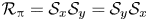 ${\mathcal {R}_{{\rm \pi} }}={\mathcal {S}_{x}}{\mathcal {S}_{y}}= {\mathcal {S}_{y}}{\mathcal {S}_{x}}$ represents the
  $180^\circ$ rotation about line
  $x=y=0$. The symmetry property of the boundary conditions could be defined accordingly. Straightforwardly, a system that behaves according to both the symmetry
  ${\mathcal {S}_{x}}$ and
  ${\mathcal {S}_{y}}$ behaves according to the symmetry
  ${\mathcal {R}_{{\rm \pi} }}$ automatically, while the symmetry
  ${\mathcal {R}_{{\rm \pi} }}$ could not guarantee the symmetry
  ${\mathcal {S}_{x}}$ nor
  ${\mathcal {S}_{y}}$.
Since the Dirichlet boundary condition applies a stronger constraint to a system as compared to the Neumann boundary condition, the type and level of symmetry would be greatly influenced by the sidewall control. In Zhang et al. (Reference Zhang, Xia, Zhou and Chen2020), a similar explanation as in Huang et al. (Reference Huang, Wang, Xi and Xia2015) was given to interpret the results in 2-D geometry. For the two-point control with  $h_c=0$, the symmetry
  ${\mathcal {S}_{x}}$ and symmetry
  ${\mathcal {S}_{y}}$ of the system are enhanced and the reversals are consequently enhanced, while for the two-point control with
  $h_c\neq 0$ only the symmetry
  ${\mathcal {R}_{{\rm \pi} }}$ is maintained while the symmetry
  ${\mathcal {S}_{x}}$ and symmetry
  ${\mathcal {S}_{y}}$ are broken. Thus the system prefers a certain orientation of LSC and correspondingly the reversal is suppressed or eliminated. However, a higher
  $Ra=10^8$ changes the results and the two-point control with
  $h_c=0$ can suppress the reversals in 2-D simulations. In addition, the newly introduced four-point control, which also satisfies
  ${\mathcal {S}_{x}},\ {\mathcal {S}_{y}}$ and
  ${\mathcal {R}_{{\rm \pi} }}$ symmetry, could also suppress reversals with proper
  $h_c$. Therefore, it is important to realize that the RBC is not always ergodic, and a system with more symmetric boundary condition does not always have the ‘intention’ to reach corresponding symmetries statistically.
With the results above, a more reasonable dynamical picture, which is similar to that in Sreenivasan et al. (Reference Sreenivasan, Bershadskii and Niemela2002), is introduced to demonstrate the reversal suppression/activation effect of sidewall control. Figure 7 shows the conceptual energy curves corresponding to different symmetry, control configurations and flow states. The two concave parts of each curve represent the two metastable clockwise and anticlockwise LSC states (potential wells) where the system tends to stay, and the bulge in the middle of each curve represents the energy barrier that keeps the system from shifting between the two main states (Sreenivasan et al. Reference Sreenivasan, Bershadskii and Niemela2002). Compared to figure 7(a), where no control is applied and the system behaves according to the symmetry  ${\mathcal {S}_{x}},\ {\mathcal {S}_{y}}$ and
  ${\mathcal {R}_{{\rm \pi} }}$, figure 7(b) is asymmetric and corresponds to the system with two-point
  $h_c>0$ control, which violates the symmetry
  ${\mathcal {S}_{x}}$ and
  ${\mathcal {S}_{y}}$ while only satisfying the
  ${\mathcal {R}_{{\rm \pi} }}$ symmetry. The energy gap where the system intends to shift from the clockwise state to the anticlockwise state is higher than that for the system to shift from the anticlockwise state to the clockwise state, indicating the system's strong preference for the clockwise state. The energy gap on the two sides of the energy barrier depends on the value of
  $h_c$ and
  $\delta _c$. Figure 7(c,d) could both represent the
  $h_c=0$ control and four-point control which satisfy the symmetry
  ${\mathcal {S}_{x}},\ {\mathcal {S}_{y}}$ and
  ${\mathcal {R}_{{\rm \pi} }}$. However, the energy barrier could be relatively lower or higher than that in figure 7(a), which depends on the specific flow state and control parameter, as discussed above. For example, the four-point control with
  $h_c=0.25$ in the 2-D case at
  $Ra=10^8$ and
  $Pr=2$ could strongly limit the growth of corner rolls and greatly increase the energy barrier, and thus corresponds to figure 7(d).

Figure 7. Conceptual energy curves of dynamical picture demonstrating reversal suppression/activation effect: (a)  $\mathcal {S}_x$,
  $\mathcal {S}_y$ and
  $\mathcal {R}_{\rm \pi}$ symmetry, corresponding to the ‘no-control’ case; (b)
  $\mathcal {R}_{\rm \pi}$ symmetry, corresponding to the present two-point control cases with
  $h_c\geq 0.05$; (c)
  $\mathcal {S}_x$,
  $\mathcal {S}_y$ and
  $\mathcal {R}_{\rm \pi}$ symmetry, corresponding to the reversal-enhancing cases with the two-point
  $h_c=0$ control and the four-point control; and (d)
  $\mathcal {S}_x$,
  $\mathcal {S}_y$ and
  $\mathcal {R}_{\rm \pi}$ symmetry, corresponding to the reversal-suppressing cases with the two-point
  $h_c=0$ control and the four-point control.
3.2. Heat transfer and kinetic energy
Owing to the sidewall control, the heat transfer through the walls occurs in two different directions, the vertical one through horizontal plates and the horizontal one through the sidewalls. The former could be quantified by the Nusselt number,
 \begin{equation} Nu(t)={-}\frac{1}{2}{{\left\langle {{\left. \frac{\partial \theta }{\partial y} \right|}_{y={-}0.5}}+{{\left. \frac{\partial \theta }{\partial y} \right|}_{y=0.5}} \right\rangle }_{x,z}}, \end{equation}
while the latter could be quantified by the Nusselt number in the horizontal direction, which can be defined similarly as
 \begin{align} N{{u}_{h}}( t )&=\frac{1}{2}{{\left\langle \int_{0}^{0.5}{\left( {{\left. \frac{\partial \theta }{\partial x} \right|}_{x=0.5}}-{{\left. \frac{\partial \theta }{\partial x} \right|}_{x={-}0.5}} \right){\,\textrm{d} y}}-\int_{{-}0.5}^{0}{\left( {{\left. \frac{\partial \theta }{\partial x} \right|}_{x=0.5}}-{{\left. \frac{\partial \theta }{\partial x} \right|}_{x={-}0.5}} \right){\,\textrm{d} y}} \right\rangle }_{z}} \nonumber\\ &=\frac{1}{2}\left[ {{\left. {{\left. {{\left\langle \text{sgn} ( y )\frac{\partial \theta }{\partial x} \right\rangle }_{y,z}} \right|}_{x=0.5}}-{{\left\langle \text{sgn} ( y )\frac{\partial \theta }{\partial x} \right\rangle }_{y,z}} \right|}_{x={-}0.5}} \right]. \end{align}
Here  $\langle Nu_h\rangle _t$ denotes the heat absorbed by the control regions below the line
  $y=0$ and also the heat injected by the control regions above the line
  $y=0$. For the two-point control, the definition of
  $Nu_h$ is consistent with that defined in Zhang et al. (Reference Zhang, Xia, Zhou and Chen2020). The time-averaged vertical Nusselt numbers
  $\langle Nu\rangle _t$ for the 2-D and quasi-2-D cases without sidewall control at
  $Ra=10^8$ and
  $Pr=2$ are
  $24.9$ and
  $32.7$, respectively, and they will be denoted as
  $\langle Nu_0\rangle _t$. The relative values of
  $\langle Nu \rangle _t$ and
  $\langle Nu_h \rangle _t$ normalized with the corresponding
  $\langle Nu_0\rangle _t$ are shown in figure 8.

Figure 8. Relative time-averaged values of vertical and horizontal Nusselt numbers given by the 2-D and quasi-2-D simulations at  $Ra=10^8$ and
  $Pr=2$. Here
  $\langle Nu_0\rangle _t$ denotes the vertical Nusselt number without sidewall control. (a) Relative time-averaged vertical Nusselt number difference
  $(\langle Nu \rangle _t-\langle Nu_0 \rangle _t)/\langle Nu_0 \rangle _t$. (b) Relative time-averaged horizontal Nusselt number
  $\langle Nu_h \rangle _t/\langle Nu_0 \rangle _t$.
According to the results shown in figure 8(a), the two-point control can enhance vertical heat transfer with  $h_c\geq 0.1$ in both 2-D and quasi-2-D cavities. However, the enhancement of vertical heat transfer is limited, with a maximum
  $4.3\,\%$ increase of
  $(\langle Nu \rangle _t-\langle Nu_0 \rangle _t)/\langle Nu_0 \rangle _t$ at
  $h_c=0.35$ in the 2-D cavity, and a maximum
  $0.6\,\%$ increase at
  $h_c=0.25$ in the quasi-2-D cavity. The curves in figure 8(a) are non-monotonic, which is similar to the phase diagram of
  $\langle Nu \rangle _t$ in Zhang et al. (Reference Zhang, Xia, Zhou and Chen2020), indicating that the underlying mechanism of the vertical heat transfer enhancement/suppression caused by control is rather complicated. Nevertheless, the reduction of vertical heat transfer by
  $h_c=0$ could be explained by larger corner rolls and consequently weaker LSC caused by control points at
  $y=0$, which is also indicated by figure 9. The four-point control is generally less capable of promoting vertical heat transport in both 2-D and quasi-2-D cavities, with significantly lower values of
  $(\langle Nu \rangle _t-\langle Nu_0 \rangle _t)/\langle Nu_0 \rangle _t$ than the corresponding two-point control cases. In the quasi-2-D cases, it is shown that the four-point control can even suppress heat transfer. Based on the above results for
  $\langle Nu \rangle _t$ and the mean time intervals between successive reversals shown in figure 5, we would like to suggest the two-point control with
  $0.1\le h_c\le 0.45$ for the 2-D cavities and
  $0.2\le h_c\le 0.45$ for the quasi-2-D cavities.

Figure 9. Time-averaged kinetic energy and the corresponding contribution from  $(1,1)$ and
  $(2,2)$ modes, in 2-D and quasi-2-D cases with
  $Ra=10^8$ and
  $Pr=2$: (a) 2-D cases and (b) quasi-2-D cases in the
  $z=0$ plane. The three dotted lines denote the corresponding time-averaged kinetic energy (black) and the contributions from the modes
  $(1,1)$ (red) and
  $(2,2)$ (blue) for the case without sidewall control.
As shown in figure 8(b),  $\langle Nu_h \rangle _t$ are generally larger than zero and mostly increasing with
  $h_c$. With heat conduction mainly with plumes in the corner rolls, the two-point control could achieve a relative
  $\langle Nu_h \rangle _t$ of
  $7.8\,\%$ at
  $h_c=0.4$ in the 2-D cavity, and
  $3.0\,\%$ at
  $h_c=0.45$ in the quasi-2-D cavity. The
  $\langle Nu_h \rangle _t$ of the four-point control is always larger than that of the corresponding two-point control. This is as expected, since there are two more control regions so that the plumes feeding corner rolls and the plumes feeding the LSC are all conducting heat with control regions, increasing the heat transfer through the sidewalls. From
  $h_c=0.4$ to
  $h_c=0.45$, the
  $\langle Nu_h \rangle _t$ decreased in 2-D geometry for both two-point and four-point control, although the control regions are closer to horizontal plates and surrounded by fluids with larger
  $|\theta |$. This is mainly because the velocity of corner rolls on the sidewalls at
  $y\approx \pm 0.45$ is relatively smaller and limits the heat transfer.
Besides heat transfer, the kinetic energy is also important in the dynamics of RBC flow. Here 2-D motion characterized by the  $(u,v)$ field in the
  $z=0$ plane is investigated, in a way similar to the analysis of the particle image velocimetry result in experiments (Chen et al. Reference Chen, Huang, Xia and Xi2019). The plane-averaged kinetic energy of
  $(u,v)$ is defined as
  $E_k(t)\triangleq \langle u(x,y,0,t)^2+v(x,y,0,t)^2 \rangle _{x,y} /2$. In order to demonstrate the distribution of
  $E_k$ from different scales, Fourier modes could be defined in the
  $x$–
$x$– $y$ plane (Chen et al. Reference Chen, Huang, Xia and Xi2019) as
 \begin{equation} \left. \begin{array}{c@{}} {{u}^{m,n}} = 2\sin ( m{\rm \pi} \tilde{x} )\cos ( n{\rm \pi} \tilde{y} ), \\ {{v}^{m,n}} ={-}2\cos ( m{\rm \pi} \tilde{x} )\sin ( n{\rm \pi} \tilde{y} ), \end{array} \right\} \end{equation}
with  $\tilde {x}\triangleq x+0.5$ and
  $\tilde {y}\triangleq y+0.5$. The expansion coefficients of
  $u(x,y,0,t)$ and
  $v(x,y,0,t)$ have certain expressions:
 \begin{equation} \left. \begin{array}{c@{}} A_{u}^{m,n}( t )={{\langle u(x,y,0,t) {{u}^{m,n}} \rangle }_{x,y}}, \\ A_{v}^{m,n}( t )={{\langle v(x,y,0,t) {{v}^{m,n}} \rangle }_{x,y}}. \end{array} \right\} \end{equation}
Therefore, the kinetic energy contributed by the  $(m,n)$ mode of
  $u$ and
  $v$ should be
 \begin{equation} {{E}_{m,n}}( t )=([ A_{u}^{m,n}( t )]^2+ [ A_{v}^{m,n}( t ) ]^2)/ 2. \end{equation}
 The kinetic energy  $E_k(t)$ together with the shares contributed by the
  $(1,1)$ and
  $(2,2)$ modes in the 2-D and quasi-2-D cases with
  $Ra=10^8$ and
  $Pr=2$ are averaged in time and shown in figure 9. For the 2-D cases, the two-point and four-point control configurations with
  $h_c\geq 0.1$ would reduce the kinetic energy
  $\langle E_k\rangle _t$, with a maximum reduction up to approximately
  $18.0\,\%$ for the two-point control, accompanied by a maximum reduction up to
  $82.1\,\%$ for
  $\langle E_{2,2}\rangle _t$. However, the reduction of the kinetic energy does not reduce, but enhances, the heat transfer in the vertical direction, as seen from figure 8(a). This is because the control with
  $h_c\geq 0.1$ could significantly enhance the LSC strength characterized by
  $\langle E_{1,1}\rangle _t$, the contribution to the kinetic energy from the
  $(1,1)$ mode, which is increased by up to
  $35\,\%$ as shown in figure 9(a). Since the large-scale LSC is more efficient in carrying heat between horizontal plates, the enhancement of LSC should be the main reason for the enhancement of heat transfer seen in figure 8(a) even though the kinetic energy is reduced. This explanation is also valid for the two-point control with
  $h_c=0$, where the reduction of
  $E_{1,1}$ is accompanied by a reduction of
  $\langle Nu\rangle _t$, although the total kinetic energy is almost unchanged.
Unlike the 2-D cases, for the quasi-2-D cases, the two-point control with  $h_c\geq 0.1$ could increase the total kinetic energy, with a maximum increase of
  $7.8\,\%$ at
  $h_c=0.3$, while the four-point control might reduce it slightly in general. With the two-point control and
  $h_c>0.1$,
  $\langle E_{1,1}\rangle _t$ could significantly increase by up to
  $83.6\,\%$ at
  $h_c=0.45$, while there is a slight decrease of
  $\langle E_{2,2}\rangle _t$. The domination of the
  $(1,1)$ mode over the
  $(2,2)$ mode could be an important reason for reversal suppression, which can also be inferred from figure 10(a,b), where the LSC, being squeezed by corner rolls in the no-control case, could become larger with the two-point control and
  $h_c=0.3$. As mentioned by Chen et al. (Reference Chen, Huang, Xia and Xi2019), in quasi-2-D convection, a slimmer LSC is convenient for corner rolls to take over and thus increases the probability of flow reversal. Therefore, although the control could not effectively force the separation of plumes feeding the corner rolls, the weakening effect on corner rolls through thermal conduction could still lead to a more stable state with stronger LSC and weaker corner rolls.
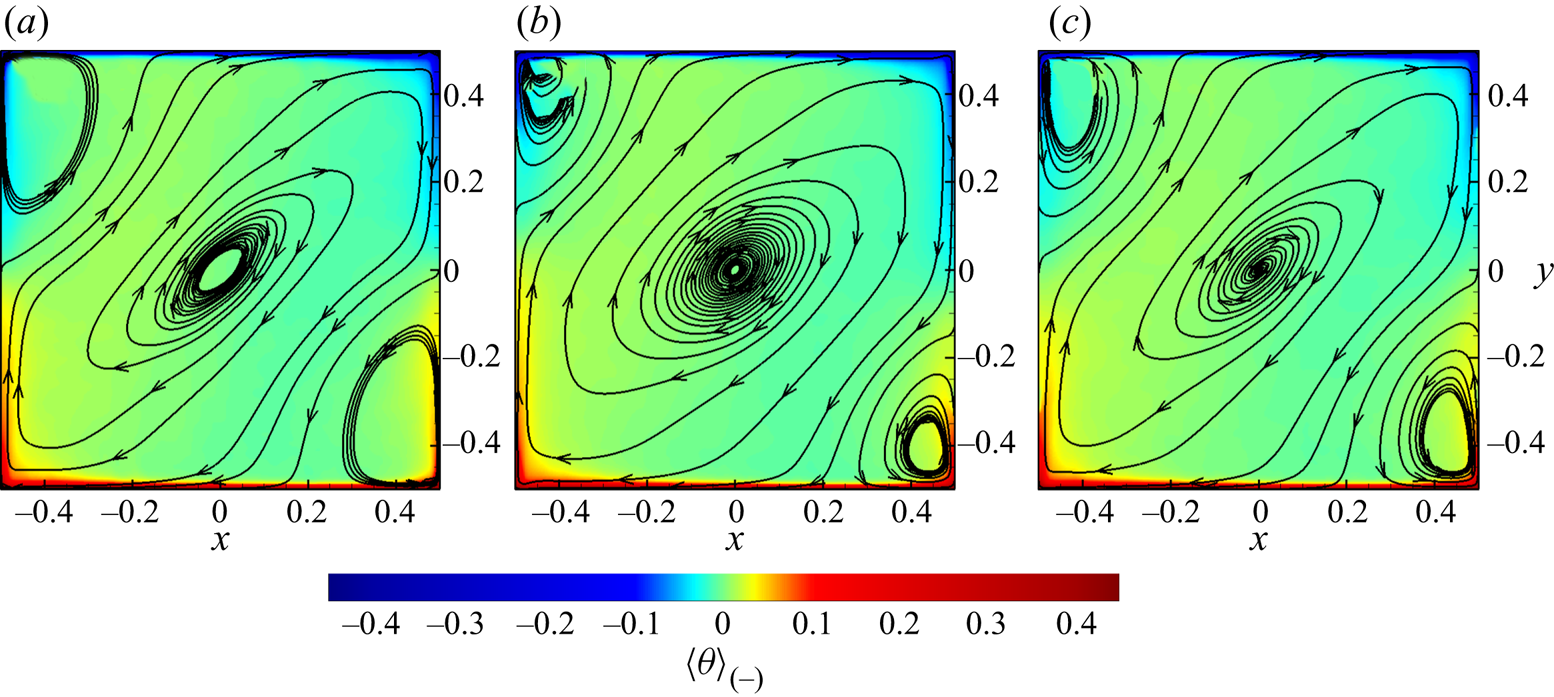
Figure 10. Temperature contours and in-plane streamlines of fields in the  $z=0$ plane and averaged during clockwise state between reversals in quasi-2-D cases with
  $Ra=10^8$ and
  $Pr=2$: (a) no control; (b) two-point control with
  $h_c=0.3$; and (c) four-point control with
  $h_c=0.3$.
Differently from those results in a 2-D cavity discussed above, the four-point control in a quasi-2-D cavity could not effectively enhance  $\langle E_{1,1}\rangle _t$, and its value at different
  $h_c$ oscillates around the reference value from the case without sidewall control. We may conclude that the LSC with four-point control has not been strengthened significantly in a quasi-2-D cavity, as shown in figure 10(c) with
  $h_c=0.3$, and thus the heat transfer in the vertical direction is comparable to (slightly less than) that from the case with adiabatic sidewalls. On the other hand, the mild decrease of
  $\langle E_{2,2}\rangle _t$ and almost unchanged
  $\langle E_{1,1}\rangle _t$, as compared to the no-control case, are consistent with the slight increase of the mean time interval between successive reversals as shown in figure 5(b), which corresponds to the slight suppression of flow reversals with the four-point control in a quasi-2-D cavity.
4. Experimental and numerical results at higher $Ra$ and $Pr$


In § 3, we have shown the numerical results at  $Ra=10^8$ and
  $Pr=2$ in 2-D and quasi-2-D cavities with different control configurations and found that the two-point control with
  $h_c>0$ can effectively suppress the flow reversals in both 2-D and quasi-2-D cavities while the four-point control can effectively suppress the flow reversals only in the 2-D cavity. In this section, we will investigate the two-point control with
  $h_c=0$ and
  $h_c=0.15$ in the quasi-2-D cavity at higher
  $Ra$ and
  $Pr$ numerically and experimentally.
Figure 11 shows the time series of  $\hat {\delta }(t)$ from the two-point controlled quasi-2-D experiments with
  $h_c=0$ and
  $h_c=0.15$ at
  $Ra\approx 1.93\times 10^8$ and
  $Pr=5.7$ as well as from the corresponding no-control case. It is seen that flow reversals happen frequently in a
  $600t_E$ time span when the sidewalls are adiabatic (without control), while the number of flow reversals reduces obviously for the two-point control with
  $h_c=0$ and
  $h_c=0.15$ in the same time span, indicating the effective suppression of flow reversals from the two-point control with
  $h_c=0$ and
  $h_c=0.15$. Our numerical results show a similar trend with increasing
  $\langle \tau \rangle$ for the two-point control with
  $h_c=0$ and
  $h_c=0.15$, as listed in table 2.

Figure 11. Plots of  $\hat {\delta }(t)$ of quasi-2-D experiments at
 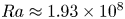 $Ra\approx 1.93\times 10^8$ and
  $Pr=5.7$ with two-point control or without control: (a) no control; (b) two-point control with
  $h_c=0$; and (c) two-point control with
  $h_c=0.15$. Green and red circles represent reversal starts and ends respectively.
Furthermore, for the two-point control with  $h_c=0$ and the no-control case, the system seems to stay in the clockwise and anticlockwise states equally, while it shows a strong preference for the clockwise state for the two-point control with
  $h_c=0.15$. The
  $\langle \tau \rangle$ values from the no-control cases and the two-point control cases with
  $h_c=0$, as well as
  $\langle \tau _-\rangle$ and
  $\langle \tau _+\rangle$ from the two-point control cases with
  $h_c=0.15$ at different
  $Ra$ are obtained and shown in figure 12. It is evident that the two-point control with
  $h_c=0.15$ could significantly suppress the flow reversals and favours the clockwise state, while the two-point control with
  $h_c=0$ can either suppress or enhance the flow reversals in the quasi-2-D experiments. At two lower
  $Ra$ (
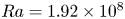 $Ra=1.92\times 10^8$ and
  $2.71\times 10^8$), the experimental results show that the two-point control with
  $h_c=0$ can slightly suppress the reversal, while at two higher
  $Ra$ (
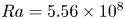 $Ra=5.56\times 10^8$ and
  $7.36\times 10^8$), it is shown that the control can enhance the flow reversal.
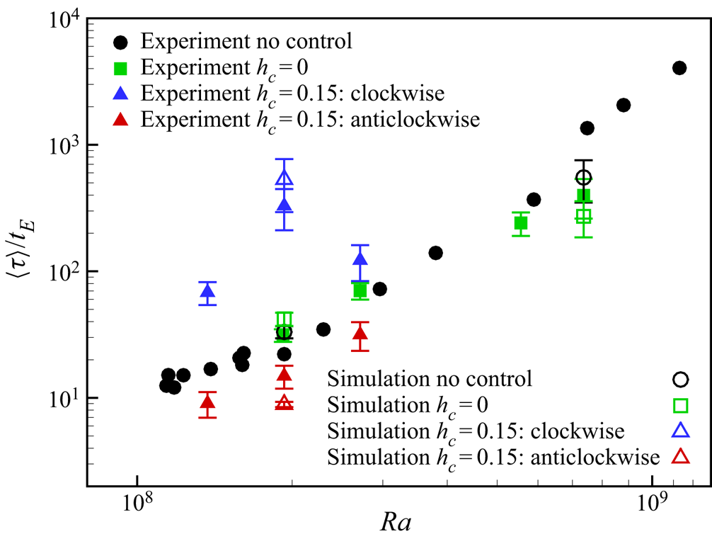
Figure 12. Mean reversal intervals from quasi-2-D experiments and simulations with two-point control configuration and without control at  $Pr=5.7$. Experimental data of no-control cases are obtained from Chen et al. (Reference Chen, Huang, Xia and Xi2019).
Simulation results show good consistency with the experiments, although their definitions of  $t_E$ are different. The relative reversal suppression/enhancement for
  $h_c=0$ control are very close between simulations and experiments at both
  $Ra=1.93\times 10^8$ and
  $Ra=7.36\times 10^8$. However, for two-point control with
  $h_c=0.15$, the clockwise state seems to exhibit greater predominance over the anticlockwise state from the simulation than the experiment at
  $Ra=1.93\times 10^8$. This is probably because the copper blocks have non-zero thermal resistance, which would not realize isothermal boundary conditions perfectly and would have less weakening effect on corner rolls as expected. Nevertheless, the experiments have proved that simply increasing thermal conductivity locally on sidewalls would have significant influence on LSC stability.
Now, we are going to explain why the two-point control with  $h_c=0$ behaves differently at
  $Ra=1.93\times 10^8$ and
  $7.36\times 10^8$. Chen et al. (Reference Chen, Huang, Xia and Xi2019) observed a new, less stable, abnormal single-roll state with substructures inside the single roll when
  $Ra$ decreases from a high value, where the classic single-roll state exists, to a relative low value, where a four-roll state can be observed. With
  $Pr=5.7$, the transition
  $Ra$ from the single-roll state to the abnormal single-roll state is around
  $2.1\times 10^8$. Figure 13 shows the averaged temperature contours and the in-plane streamlines of flow fields in the
  $z=0$ plane from the no-control cases with
  $Ra=1.93\times 10^8$ and
  $Ra=7.36\times 10^8$, and it is seen that the system shows the abnormal single-roll state at
  $Ra=1.93\times 10^8$, while it reveals the single-roll state at
  $Ra=7.36\times 10^8$, which are consistent with the experimental results in Chen et al. (Reference Chen, Huang, Xia and Xi2019). According to Chen et al. (Reference Chen, Wang and Xi2020), the reversal of the abnormal single-roll state is dominated by the instability of LSC, which is highly squeezed to be dumbbell-shaped by the corner rolls. Since the structural stability of LSC is already low for the abnormal single-roll state, the
  $h_c=0$ control may not further reduce the LSC stability, but could instead reduce the perturbations on LSC from plumes, resulting in a suppression of reversals. When
  $Ra$ is higher and the flow turns into the single-roll state, whose reversal is dominated by the growth of corner rolls (Chen et al. Reference Chen, Wang and Xi2020), the presence of
  $h_c=0$ control could raise the height of the corner rolls and increase the instability of LSC, consequently enhancing reversals.

Figure 13. Averaged temperature contours and in-plane streamlines of fields in the  $z=0$ plane from the simulations of the no-control quasi-2-D cases with
  $Pr=5.7$: (a)
  $Ra=1.93\times 10^8$ and (b)
  $Ra=7.36\times 10^8$. The averaging is performed on the condition that the system is in the clockwise state.
5. Conclusion
In the present paper, the local sidewall control on 2-D and quasi-2-D RBC is studied numerically and experimentally. In addition to the two-point control configuration studied by Zhang et al. (Reference Zhang, Xia, Zhou and Chen2020), another configuration with four control regions and higher symmetry property is also simulated and compared with those two-point control cases. With a fixed width of the control region  $\delta _c=0.05$ at
  $Ra=10^8$ and
  $Pr=2$, the direct numerical simulation results show that both the two-point and four-point controls can effectively suppress the flow reversals when
  $h_c\geq 0.05$ in the 2-D cavity, while only the two-point control shows effective suppression on the flow reversal with
  $h_c\geq 0.05$ in the quasi-2-D cavity. The effect of the four-point control in the quasi-2-D cavity is rather limited. Further analysis shows that the two-point control with
  $h_c\geq 0.05$ will favour a clockwise LSC state over the anticlockwise LSC state in both 2-D and quasi-2-D cavities. In addition, the two-point control with
  $h_c\geq 0.1$ can significantly increase the energy of LSC according to the mode decomposition and consequently increase the vertical heat transfer. More specifically, in the 2-D cavity some medium
  $h_c$ is optimal for reversal suppression, but in the quasi-2-D cavity larger
  $h_c$ seems to be more efficient in reversal suppression. These results not only reveal the superior suppression effect of the two-point control over the four-point control, but also show the differences between 2-D and quasi-2-D simulations.
Besides the discussions on the reversal suppression/enhancement effect from different control configurations, a conceptual picture is presented based on symmetry: the two-point control with  $h_c>0$ breaks the symmetry about planes
  $x=0$ and
  $y=0$, and favours a specific LSC orientation; while
  $h_c=0$ control and four-point control increase the level of symmetry but its suppression/enhancement on reversals should be decided together with specific flow state. Whether a symmetry-preserving control increases or reduces the LSC stability still remains an open question.
The effect of the two-point control at  $Pr = 5.7$ with higher
  $Ra$ up to
  $7.36\times 10^8$ is also investigated in the quasi-2-D cavity, both numerically and experimentally, to explore the realizability and efficiency of the control strategy in real flows. Simulations and experiments with the same parameters show good consistency, suggesting that the present control strategy is practicable and efficient for real flow apparatus. Furthermore, the results show that the two-point control with
  $h_c= 0.15$ can effectively suppress the flow reversal while the two-point control with
  $h_c= 0$ can either suppress or activate the reversals depending on
  $Ra$. With fixed
  $Pr=5.7$ and
  $Ra= 1.93\times 10^8$, the control will suppress the flow reversals while it can activate the reversals at higher
  $Ra = 7.36 \times 10^8$. We attribute the discrepancies at different
  $Ra$ to the different flow topology. Since the flow topology also depends on
  $Pr$, further studies may be performed to investigate the
  $Pr$ and
  $Ra$ effects on the two-point control with different
  $h_c$.
Acknowledgements
The numerical simulations were finished at National Supercomputer Center in Guangzhou (Tianhe-2A), China.
Funding
This work was supported by the National Science Foundation of China (NSFC grant nos. 11822208, 11988102, 11772297, 91852205, 11825204 and 11772259) and Shenzhen Science and Technology Program (grant no. KQTD20180411143441009).
Declaration of interest
The authors report no conflict of interest.