


1 Introduction
Gravity currents are nearly horizontal flows driven by lateral density gradients (Simpson Reference Simpson1982, Reference Simpson1997). They play a key role in the transport of scalars in a range of environmental settings, including dense inflows into lakes (Fischer & Smith Reference Fischer and Smith1983; Hogg et al. Reference Hogg, Marti, Huppert and Imberger2013; Cortés et al. Reference Cortés, Fleenor, Wells, de Vicente and Rueda2014a), snow avalanches (Sovilla, McElwaine & Köhler Reference Sovilla, McElwaine and Köhler2018), katabatic winds down mountain faces and valleys (Samothrakis & Cotel Reference Samothrakis and Cotel2006b), turbidity currents and mudslides (MacIntyre et al. Reference MacIntyre, Flynn, Jellison and Romero1999; Marti & Imberger Reference Marti and Imberger2008), volcanic lava gravity currents (Huppert & Dade Reference Huppert and Dade1998) and effluent discharges (Rueda, Fleenor & de Vicente Reference Rueda, Fleenor and de Vicente2007; Baines Reference Baines2008; Meiburg & Kneller Reference Meiburg and Kneller2010; Hodges, Furnans & Kulis Reference Hodges, Furnans and Kulis2011). When an inclined gravity current descends down a slope, it entrains ambient fluid and is gradually diluted as it flows (Ellison & Turner Reference Ellison and Turner1959; Hebbert et al. Reference Hebbert, Patterson, Loh and Imberger1979; Dallimore, Imberger & Ishikawa Reference Dallimore, Imberger and Ishikawa2002; Fernandez & Imberger Reference Fernandez and Imberger2006; Cenedese & Adduce Reference Cenedese and Adduce2010). Gravity currents propagating in homogeneous environments have been extensively studied in the laboratory, leading to well-developed characterizations of the entrainment and frontal structure (Benjamin Reference Benjamin1968; Britter & Simpson Reference Britter and Simpson1978; Simpson & Britter Reference Simpson and Britter1979; Britter & Linden Reference Britter and Linden1980; Hallworth et al. Reference Hallworth, Huppert, Phillips and Sparks1996; Odier, Chen & Ecke Reference Odier, Chen and Ecke2012, Reference Odier, Chen and Ecke2014), mixing and entrainment at the interface (Krug et al. Reference Krug, Holzner, Lüthi, Wolf, Kinzelbach and Tsinober2015) and propagation along spatially varying bathymetry (Negretti, Flòr & Hopfinger Reference Negretti, Flòr and Hopfinger2017).
When the receiving ambient is stratified, the fate and transport of the gravity current become more complex than in a homogeneous environment (Monaghan Reference Monaghan2007). In the stratified case, the gravity current will insert itself into the ambient at a depth where its fluid is neutrally buoyant (Fischer et al. Reference Fischer, Koh, List, Koh, Imberger and Brooks1979; Turner Reference Turner1986; Chapra Reference Chapra1997; Baines Reference Baines2001). Researchers have examined the structure and propagation of purely intrusive gravity currents in stratified ambients using both theoretical analyses and laboratory experiments (Holyer & Huppert Reference Holyer and Huppert1980; Britter & Simpson Reference Britter and Simpson1981; Lowe, Linden & Rottman Reference Lowe, Linden and Rottman2002; Flynn & Sutherland Reference Flynn and Sutherland2004; Sutherland, Kyba & Flynn Reference Sutherland, Kyba and Flynn2004; Cheong, Kuenen & Linden Reference Cheong, Kuenen and Linden2006), as well as gravity currents propagating at the base of a stratified ambient (Maxworthy et al. Reference Maxworthy, Leilich, Simpson and Meiburg2002; Ungarish & Huppert Reference Ungarish and Huppert2002). In two-layer stratifications, such as below the wind mixed layer in the ocean, a gravity current will either intrude at the pycnocline, if it is lighter than the lower layer, or split into an intrusion at the pycnocline and a gravity current descending beneath the lower ambient layer, if it contains fluid denser than the lower layer (Monaghan et al. Reference Monaghan, Cas, Kos and Hallworth1999; Samothrakis & Cotel Reference Samothrakis and Cotel2006b; Monaghan Reference Monaghan2007; Wells & Wettlaufer Reference Wells and Wettlaufer2007; Mott & Woods Reference Mott and Woods2009; Cortés et al. Reference Cortés, Fleenor, Wells, de Vicente and Rueda2014a; Cortés, Rueda & Wells Reference Cortés, Rueda and Wells2014b).
Monaghan et al. (Reference Monaghan, Cas, Kos and Hallworth1999) examined a dense gravity current descending into a two-layer stratified system and observed solitary internal wave generation and the splitting of the gravity current, but the splitting was not quantified or predictable. In similar experiments, Samothrakis & Cotel (Reference Samothrakis and Cotel2006a,Reference Samothrakis and Cotelb) investigated the changes in vorticity and velocity for a gravity current before and after the pycnocline, for both finite-volume and continuous releases. They found that both quantities increased after impinging on the pycnocline for supercritical gravity currents and decreased for subcritical gravity currents. Cortés et al. (Reference Cortés, Rueda and Wells2014b) developed a predictive framework for the splitting of a gravity current using both the density and velocity profile of the gravity current before the impingement on the pycnocline, and found good agreement with numerical experiments in Cortés et al. (Reference Cortés, Wells, Fringer, Arthur and Rueda2015). However, in many environmental flows the exact density and velocity profiles are not known.
Motion in the ambient fluid has also been shown to exert a significant influence on the behaviour of the gravity current (Ellison & Turner Reference Ellison and Turner1959; Fischer & Smith Reference Fischer and Smith1983). For example, when there is a counter-flow, as occurs in estuarine salt wedges (Simpson Reference Simpson1997), the gravity current can be arrested or reversed and its thickness can be modified (Ellison & Turner Reference Ellison and Turner1959; Britter & Simpson Reference Britter and Simpson1978; Hallworth, Hogg & Huppert Reference Hallworth, Hogg and Huppert1998). In addition, the collision of two gravity currents has been shown to generate reflected bores (Shin Reference Shin2001). Finally, recent experiments on gravity currents propagating beneath free-surface waves showed that the gravity current motion was dominated by the gravity current density, with Stokes drift caused by the surface waves being only a second-order effect (Robinson, Eames & Simons Reference Robinson, Eames and Simons2013). Little research has been done on gravity currents propagating into turbulent environments. Linden & Simpson (Reference Linden and Simpson1986) examined gravity currents in fluids with background turbulence generated by rising bubbles. They found that in the presence of strong background turbulence the head of the gravity current would not form and the advance of the gravity current was best modelled as a turbulent diffusion process rather than advection driven by density gradients. Gravity currents have also been shown to drive ambient motion by radiating internal waves in stratified fluids (Monaghan et al. Reference Monaghan, Cas, Kos and Hallworth1999; Maxworthy et al. Reference Maxworthy, Leilich, Simpson and Meiburg2002; Ungarish & Huppert Reference Ungarish and Huppert2002; Flynn & Linden Reference Flynn and Linden2006; Maurer & Linden Reference Maurer and Linden2014).
In addition to naturally occurring gravity currents, there is now an increasing need to consider the fate of anthropogenic gravity currents in the coastal environment, such as the discharge of brine effluents from seawater desalination facilities. These may be continuous or finite-volume releases, depending on the operating procedures of the facility (Roberts, Johnston & Knott Reference Roberts, Johnston and Knott2010; Hodges et al. Reference Hodges, Furnans and Kulis2011; Lattemann & Amy Reference Lattemann and Amy2013; Missimer & Maliva Reference Missimer and Maliva2017). The extent to which brine plumes from these facilities have an impact on the coastal ocean remains very uncertain (Fernández-Torquemada et al. Reference Fernández-Torquemada, Gónzalez-Correa, Loya, Ferrero, Díaz-Valdés and Sánchez-Lizaso2009; Jenkins et al. Reference Jenkins, Paduan, Roberts, Schlenk and Weis2012), but they are likely to have significant ecological and economic consequences (Kvitek, Conlan & Iampietro Reference Kvitek, Conlan and Iampietro1998). Fundamental understanding of the mixing and transport of the plume in ambient receiving waters, which typically have strong internal wave action, is critical for predicting the concentrations of brine and chemical additives in the plume and the reduction in oxygen at the seabed beneath the brine (Hodges et al. Reference Hodges, Furnans and Kulis2011).
Although we are studying a quiescent ambient stratification, many stratified natural and engineered systems contain internal waves and seiches that are a significant source of kinetic energy that may affect the downslope transport of gravity currents (Fischer & Smith Reference Fischer and Smith1983; Turner Reference Turner1986; Masunaga, Fringer & Yamazaki Reference Masunaga, Fringer and Yamazaki2016). Fischer & Smith (Reference Fischer and Smith1983) found in their field study that internal wave motions were responsible for transporting a portion of an initially negatively buoyant river inflow to the surface. Internal waves incident on slopes have been extensively studied in the laboratory (Troy & Koseff Reference Troy and Koseff2005b; Hult, Troy & Koseff Reference Hult, Troy and Koseff2011; Moore, Koseff & Hult Reference Moore, Koseff and Hult2016), numerical simulations (Venayagamoorthy & Fringer Reference Venayagamoorthy and Fringer2007; Arthur & Fringer Reference Arthur and Fringer2014) and the field (Davis & Monismith Reference Davis and Monismith2011; Walter et al. Reference Walter, Woodson, Arthur, Fringer and Monismith2012), and have been shown to greatly enhance vertical mixing when they break and shoal, resulting in a turbulent bolus propagating upslope. Recent experiments by Hogg et al. (Reference Hogg, Pietrasz, Egan, Ouellette and Koseff2016, Reference Hogg, Egan, Ouellette and Koseff2017) have demonstrated that a single oncoming internal wave can reduce the downslope mass flux of a gravity current by up to 40 %.
Although there is ultimately a need to understand the interaction between gravity currents and breaking internal waves on slopes, in this paper we focus on the zero-order question of the dynamics of gravity currents propagating into a stratified two-layered system with the goal of answering the following questions:
(i) How does the gravity current split, based on the initial conditions for the gravity current and the receiving ambient stratification?
(ii) How does the pycnocline in a two-layer stratification respond to different gravity currents?
In the following, we first provide details of our experimental facility and procedures, and an overview of the non-dimensional parameters that give the theoretical backdrop for our analyses in § 2. In § 3 we present the results from our experiments as well as a discussion of these results. Overall conclusions derived from our study are given in § 4.
2 Experimental methods
2.1 Facility
A series of experiments were performed in the Stratified Flow Facility in The Bob and Norma Street Environmental Fluid Mechanics Laboratory at Stanford University (see Troy & Koseff (Reference Troy and Koseff2005a) and Moore et al. (Reference Moore, Koseff and Hult2016) for more details). A schematic of the experimental set-up is shown in figure 1. The facility consists of an enclosed rectangular tank 488 cm long, 60 cm tall and 30 cm wide fitted with an inclined slope of  $6^{\circ }$ caulked to the side of the tank. A lock that is 56 cm long and 10.6 cm deep at the top of the incline allows the gravity current fluid to be held in isolation from the rest of the tank before the experiment begins.

Figure 1. Schematic of the facility and measurement instrumentation. The blue box shows the region where PLIF was conducted, and the four red boxes show the fields of view of the cameras used to image the tracer dye.
2.2 Procedure
A two-layer stratification was prepared following the methodology of Moore et al. (Reference Moore, Koseff and Hult2016), using a floating diffuser to achieve an overall density difference of  $\unicode[STIX]{x0394}\unicode[STIX]{x1D70C}/\unicode[STIX]{x1D70C}_{0}=2(\unicode[STIX]{x1D70C}_{2}-\unicode[STIX]{x1D70C}_{1})/(\unicode[STIX]{x1D70C}_{2}+\unicode[STIX]{x1D70C}_{1})=1.2\,\%$ between the two ambient layers. The density of the upper layer was close to that of fresh water, although a small amount of NaCl was added to improve the performance of the conductivity probe (Precision Measurements Engineering, model 125) used to measure densities. The probe had a fast-response conductivity sensor (-3 dB at approximately 800 Hz) and fast thermistor (7 ms response time), allowing for accurate density measurements, and was traversed vertically at a speed of
  $10~\text{cm}~\text{s}^{-1}$. The upper-layer density was
  $\unicode[STIX]{x1D70C}_{1}\approx 1001~\text{kg}~\text{m}^{-3}$, and the lower layer was set to a density of
  $\unicode[STIX]{x1D70C}_{2}\approx 1013~\text{kg}~\text{m}^{-3}$. The gravity current fluid that was initially in the lock was set to a density
  $\unicode[STIX]{x1D70C}_{3}$ ranging from 1017 to
  $1038~\text{kg}~\text{m}^{-3}$. All the fluid used in the experiments was allowed to equilibrate to the ambient laboratory temperature prior to the experiments to remove any temperature variability that could affect the density.
The upper- and lower-layer heights were kept constant at  $h_{1}=21~\text{cm}$ and
  $h_{2}=27.5~\text{cm}$, respectively, for all experiments, and the distance from the lock to the pycnocline was 100 cm as measured along the incline. Prior to initiating the experiments, the pycnocline region of intermediate density between the ambient layers was sharpened using a thin slotted pipe as described in Troy & Koseff (Reference Troy and Koseff2005a). The interfacial thickness was calculated from a vertical density profile taken with the conductivity probe mounted on a vertical traverse as the thickness over which 99 % of the density variations occurred, consistent with Fringer & Street (Reference Fringer and Street2003) and Troy & Koseff (Reference Troy and Koseff2005a), and was held constant for all experiments at
  $1.4\pm 0.2~\text{cm}$.
While stratifying the tank, the lock was closed off so that there was no mixing of the gravity current fluid with the tank fluid. At the start of the experiment, the lock containing the gravity current was opened sharply to a prescribed gate opening height ( $h_{0}$) allowing the gravity current to form on the slope. The partial gate opening is not an issue for the reproducibility of the experiments, and we found a very consistent relationship between the gravity current depth
  $h_{c}$ and the gate opening height
  $h_{0}$.
The volume of the gravity current was kept constant for all experiments at  $16\,000~\text{cm}^{3}$, similar to that of the experiments of Samothrakis & Cotel (Reference Samothrakis and Cotel2006a) and other experiments summarized in table 3 of Samothrakis & Cotel (Reference Samothrakis and Cotel2006a). Vertical density profiles were taken at the downstream end of the tank where the bottom slope is horizontal both before and after the gravity current release. Profiling was continued for 2 h following the release of the gravity current to ensure that no horizontal gradients in the density field were present. A sampling port allowed density measurements to be taken at the bottom of the tank, as the probe was limited in its traversal to a few centimetres above the bottom. A hyperbolic tangent fit was used to extrapolate the bottom portion of the density profile to the measured density while enforcing the no-flux boundary condition on the density profile.
2.3 Planar laser-induced fluorescence
Planar laser-induced fluorescence (PLIF) was used to obtain the velocity, density and overall structure of the gravity current before it reached the pycnocline. The fluid was seeded with a laser-fluorescent dye (rhodamine 6G) with a Schmidt number similar to that of the salt used to stratify the fluid ( $Sc=\unicode[STIX]{x1D708}/\unicode[STIX]{x1D705}$ of 600–1200 and 700, respectively, where
  $\unicode[STIX]{x1D708}$ is the kinematic viscosity and
  $\unicode[STIX]{x1D705}$ is the molecular diffusivity). The concentration of the laser-induced fluorescence dye was then directly related to the salinity field (Rehmann Reference Rehmann1995).
A computer-controlled scanning mirror was used to generate a light sheet with a width of approximately 0.5 mm at its thinnest from a Nd : YAG laser beam, illuminating the dye in a two-dimensional plane along the centreline of the tank. The imaging domain is shown in figure 1, and was selected so that measurements of the gravity current could be taken before its interaction with the pycnocline. Images were acquired using a  $2048\times 2048$ pixel CCD camera (Redlake ES 4.0 with a SIGMA 30 mm F1.4 DC HSM lens), and the spatial resolution was 0.2 mm. The pixel intensity from the imaging was converted to dye concentration and then to density using the calibration methodology of Crimaldi & Koseff (Reference Crimaldi and Koseff2001) and Troy & Koseff (Reference Troy and Koseff2005a). Images were acquired at a frame rate of 7.5 Hz. Using this approach, the density, frontal speed and height of the gravity current head could be measured. The frontal speed of the gravity current was determined in a manner similar to that of Simpson (Reference Simpson1997), Venayagamoorthy & Fringer (Reference Venayagamoorthy and Fringer2007) and Moore et al. (Reference Moore, Koseff and Hult2016). Figure 2 shows a set of processed images acquired with PLIF showing the density gradients in the gravity current as well as the evolution of the frontal position of the gravity current.

Figure 2. Image sequence of a gravity current propagating downslope. Images are shown at 0.53 s intervals. The frontal position of the gravity current moves at a constant speed, as indicated by the dashed straight line.
2.4 Flow visualization
An array of four cameras (Basler acA2040-90um with TAMRON 16 mm F1.8 lenses, 0.8 mm resolution) was set up along the length of the tank (denoted by four red boxes in figure 1) to capture the progression of the gravity current, as well as other flow features, along the entirety of the tank, as opposed to the limited spatial extent of the PLIF camera. Dye (McCormick® Food Colouring) was added to the different ambient layers and the gravity current to distinguish the different fluids. Although the density of the fluid could not be extracted from these images, the gravity current speed and any pycnocline movement could be quantified by processing them. The image acquisition was synchronized between all the cameras using an external function generator.
2.5 Non-dimensional parameters
The Richardson number,  $Ri$, expressing the competition between buoyancy and shear, is typically used to characterize gravity current dynamics. However, various forms of the Richardson number appear in the literature and are appropriate for different situations. In the case of a gravity current released into a homogeneous ambient, Ellison & Turner (Reference Ellison and Turner1959) and Britter & Linden (Reference Britter and Linden1980) found that the gravity current can be characterized by a Richardson number defined as
 $$\begin{eqnarray}Ri=\frac{g_{13}^{\prime }h\cos \unicode[STIX]{x1D703}}{U^{2}},\end{eqnarray}$$
 where  $g_{13}^{\prime }=g(\unicode[STIX]{x1D70C}_{3}-\unicode[STIX]{x1D70C}_{1})/\unicode[STIX]{x1D70C}_{0}$ is the reduced gravity calculated with the gravity current and ambient density and
  $h$ and
  $U$ are the height and mean velocity of the gravity current. The entrainment, or the rate at which the gravity current head grows, is a function of this Richardson number (Ellison & Turner Reference Ellison and Turner1959). This Richardson number can be also interpreted as a densimetric Froude number with the relation
  $Fr=Ri^{-2}$ to describe the criticality of the gravity current. The gravity currents in the present study are all subcritical by this
  $Fr$ criterion, whereas other studies such as Cortés et al. (Reference Cortés, Rueda and Wells2014b) examined both supercritical and subcritical gravity current regimes.
Wallace & Sheff (Reference Wallace and Sheff1987) proposed a different form of the Richardson number to predict and characterize the fate of a buoyant plume in a two-layer stratification. This formulation of  $Ri$ relates both the depth of the ambient layer into which the gravity current is released and the strength of the ambient stratification to the buoyancy flux of the gravity current, and is given by
 $$\begin{eqnarray}Ri_{\unicode[STIX]{x1D70C}}=\frac{g_{12}^{\prime }h_{1}}{B^{2/3}},\end{eqnarray}$$
 where  $g_{12}^{\prime }=g(\unicode[STIX]{x1D70C}_{2}-\unicode[STIX]{x1D70C}_{1})/\unicode[STIX]{x1D70C}_{0}$ is the reduced gravity over the ambient stratification and
  $B=g_{13}^{\prime }Q/b$ is the buoyancy flux per unit width, where
  $b$ is the width. For a negatively buoyant gravity current, shallow-water theory and dam-break theory predict the depth of the fluid leaving the lock gate as
  $h_{c}=4/9h_{0}$ and the average velocity as
  $U_{c}=2/3(g_{13}^{\prime }h_{0})^{1/2}$ (Acheson Reference Acheson1990), giving the buoyancy flux per width as
  $B=g_{13}^{\prime }h_{c}U_{c}=8/27(g_{13}^{\prime }h_{0})^{3/2}$. Britter & Linden (Reference Britter and Linden1980) found that the frontal speed of the gravity current is
  $U_{f}/B^{1/3}=1.5\pm 0.2$ independent of the slope for inclines in the range
  $5^{\circ }\leqslant \unicode[STIX]{x1D703}\leqslant 90^{\circ }$. Monaghan et al. (Reference Monaghan, Cas, Kos and Hallworth1999) found that
  $U_{f}/B^{1/3}=1.0\pm 0.1$ for slopes between
  $20^{\circ }$ and
  $90^{\circ }$, whereas Samothrakis & Cotel (Reference Samothrakis and Cotel2006b) found that
  $U_{f}/B^{1/3}=1.6\pm 0.3$ for a slope of
  $6^{\circ }$. In our experiments, we find that
  $U_{f}/B^{1/3}=0.93\pm 0.1$, more consistent with the results of Monaghan et al. (Reference Monaghan, Cas, Kos and Hallworth1999). Our calculations of
  $U_{f}/B^{1/3}$ agree with values found in the literature suggesting that the buoyancy flux was calculated correctly, and that shallow-water theory holds. While the partial gate opening certainly affects the buoyancy flux, the effects are well captured by the theory, and as stated above are highly reproducible.
Using only the initial conditions of the experiment, we can also define a Grashof number describing the ratio of the buoyancy of the gravity current to viscous forces as
 $$\begin{eqnarray}Gr=\frac{h_{0}\sqrt{g_{13}^{\prime }h_{0}}}{\unicode[STIX]{x1D708}}.\end{eqnarray}$$
 A larger Grashof number indicates that the gravity current flow is dominated by buoyancy-driven inertia as opposed to viscous drag. In our experiments,  $Gr$ ranged from
  $3.2\times 10^{3}$ to
  $1.9\times 10^{4}$ so that the motion of the gravity current is indeed dominated by buoyancy. The Reynolds number
 $$\begin{eqnarray}Re=\frac{hU_{f}}{\unicode[STIX]{x1D708}}\end{eqnarray}$$
 of the gravity current can also be calculated using the characteristic height and frontal speed of the gravity current, and ranged from  $1.8\times 10^{3}$ to
  $9.7\times 10^{3}$ in our experiments.
3 Results
We focus on addressing two fundamental questions in this paper. First, as the gravity current passes through the density interface, does it split in the manner described by Cortés et al. (Reference Cortés, Rueda and Wells2014b) as a function of the Richardson number of the current? Second, what is the behaviour of the interface itself as the gravity current passes through it? In the following, we address each question in turn.
3.1 Behaviour of the gravity current
We first describe our results in a qualitative way, and subsequently use a more quantitative analysis of the centre of mass of the water column to assess how the current distributes itself after passing through the interface. The experimental conditions are given in table 1. The first nine runs were each conducted twice, once using PLIF to capture the gravity current in the pre-pycnocline region of the incline and once with an array of cameras to track the subsequent movement of the pycnocline. We performed the runs separately because the tracer dye used in the latter experiments interferes with the laser-induced fluorescence in the PLIF experiments.
Table 1. Parameters for the different experimental runs, where  $\unicode[STIX]{x1D70C}_{1}$ and
  $\unicode[STIX]{x1D70C}_{2}$ are the densities of the upper and lower ambient layers,
  $\unicode[STIX]{x1D70C}_{3}$ is the gravity current density and
  $h_{0}$ is the gate opening at the lock. Here
  $Ri_{\unicode[STIX]{x1D70C}}$,
  $Gr$ and
  $Re$ are the Richardson number, Grashof number and Reynolds number of the current, respectively (see text for definitions).

The propagation of the gravity current through the top ambient layer is similar to the homogeneous ambient case that has been extensively studied by, among others, Britter & Simpson (Reference Britter and Simpson1978), Britter & Linden (Reference Britter and Linden1980) and Simpson (Reference Simpson1997), where rapid entrainment due to Kelvin–Helmholtz instabilities at the interface between the gravity current and ambient fluid reduces the overall density in the gravity current as it propagates down the slope. PLIF images, as depicted in figure 2, show that the gravity current head consists of an array of ever-evolving vortices due to the constant baroclinic torque production of vorticity through the misalignment of the density and pressure gradient as well as the initial vorticity produced in the current boundary layer. The tail of the gravity current moves faster than the head of the current, contributing an additional source of growth of the head (Monaghan Reference Monaghan2007). As with experiments of Monaghan et al. (Reference Monaghan, Cas, Kos and Hallworth1999), a return bore of the upper-layer fluid is generated in the gravity current lock, but the head of the gravity current reaches the pycnocline before the bore affects the flow. Furthermore, the draining flow observed in the last stages of the gravity current fluid leaving the lock does not influence the interaction of the gravity current head with the pycnocline, which occurs well before this.

Figure 3. Splitting of the gravity current for different experimental conditions: (a)  $Ri_{\unicode[STIX]{x1D70C}}=8.1$, showing a strong interflow; (b)
  $Ri_{\unicode[STIX]{x1D70C}}=3.7$, showing a splitting of the gravity current into an underflow and interflow; and (c)
  $Ri_{\unicode[STIX]{x1D70C}}=2.3$, where the gravity current is predominantly an underflow.
Upon reaching the pycnocline, we typically observe that the gravity current splits into two parts: one that penetrates the pycnocline and continues to propagate downslope (figure 3c), and one that inserts itself into the ambient stratification at the pycnocline (figure 3a) (Samothrakis & Cotel Reference Samothrakis and Cotel2006b; Monaghan Reference Monaghan2007). Given the density structure of the water column, the part of the gravity current with a density exceeding that of the lower layer proceeds downslope as an underflow and the part with a density less than that of the lower layer flows horizontally as an interflow. These flows are referred to as hyperpycnal and mesopycnal flows in sedimentology (Mulder & Alexander Reference Mulder and Alexander2001). Through entrainment and mixing, an underflow can change the ambient stratification in the lower layer, whereas an interflow will result in a thickening of the pycnocline. In the following sections we quantify the amount of underflow and interflow for different experimental cases, and the subsequent pycnocline motions in response to an underflow or interflow.
3.1.1 Splitting of the gravity current
The vertical density profiles before and after the experiment can be used to quantify the extent of underflow or interflow. We consider multiple hypothetical outcomes, and compare those profiles to the actual experimentally measured profiles. Neglecting the case where the gravity current inserts into the ambient as a buoyant plume (in which the dynamics of the ambient two-layer stratification remains unaffected), three distinct limiting cases are possible and are discussed in detail below.
(a) Full interflow
In the case where the entrainment of the upper-layer fluid into the gravity current is significant, so that the density of the gravity current when it reaches the interface is less than that of the lower layer but slightly more than that of the upper layer, the entire volume of the gravity current will insert itself horizontally along the ambient pycnocline. In this full interflow scenario, the vertical extent of the ambient lower layer would not change, but the region of intermediate densities between the two layers will be thickened. This is shown schematically by the orange line with diamonds in figure 4.

Figure 4. Comparison of measured and hypothetical vertical density profiles for (a)  $Ri_{\unicode[STIX]{x1D70C}}=1.9$ and (b)
  $Ri_{\unicode[STIX]{x1D70C}}=6.4$. The horizontal lines indicate the centre of mass (
 $M_{c}$) for each density profile. The symbols have been added for clarification and do not reflect the sampling resolution.
(b) Fully mixed underflow
If the density of the gravity current remains close to its initial density as it reaches the pycnocline but then proceeds to mix completely with the lower ambient layer, the result is a fully mixed underflow. The lower-layer density is increased due to the additional density excess from the gravity current. The pycnocline thickness would be unaffected but it would be displaced upwards from the volumetric addition to the lower layer. This is shown schematically by the green line with asterisks in figure 4.
(c) Pure underflow
If the gravity current were immiscible with the ambient and therefore did not mix with either of the ambient layers, the current would insert itself with its original density at the bottom of the tank. This is the absolute lowest limit where a negatively buoyant gravity current could settle. In this case, the pycnocline thickness would remain unchanged but it would be displaced upwards from the underflow. This is shown schematically by the blue line with squares in figure 4.
(d) Experiments
Figure 4 shows the vertical density profiles for two separate inflow cases,  $Ri_{\unicode[STIX]{x1D70C}}=1.9$ and
  $Ri_{\unicode[STIX]{x1D70C}}=6.4$, along with the hypothetical profiles described above. In the
  $Ri_{\unicode[STIX]{x1D70C}}=1.9$ case, the initial density of the gravity current is higher than that of the
  $Ri_{\unicode[STIX]{x1D70C}}=6.4$ case. Therefore, the gravity current signature in the immiscible underflow case shows a higher density in the
  $Ri_{\unicode[STIX]{x1D70C}}=1.9$ case than in the
  $Ri_{\unicode[STIX]{x1D70C}}=6.4$ case. Similarly, the lower-layer density in the fully mixed underflow case is higher for the
  $Ri_{\unicode[STIX]{x1D70C}}=1.9$ case than for the
  $Ri_{\unicode[STIX]{x1D70C}}=6.4$ case. In both measured final density profiles (red line with circles), the excess density from the gravity current underflow can be seen at the bottom of the profiles. Below the pycnocline in the
  $Ri_{\unicode[STIX]{x1D70C}}=1.9$ case, the excess is present at around 20 cm, compared to around 15 cm in the
  $Ri_{\unicode[STIX]{x1D70C}}=6.4$ case. The density of the gravity current at the bottom has been reduced compared to its initial density due to entrainment while propagating through the ambient, consistent with experimental observations by Baines (Reference Baines2001) of gravity currents flowing into a continuous stratification.
The red lines with circles in figure 4 show the actual resultant density profiles for the two different flow cases superimposed on the theoretical profiles discussed above. The  $Ri_{\unicode[STIX]{x1D70C}}=6.4$ case had a lower
  $g_{13}^{\prime }$ and buoyancy flux, which suggests that, given that the velocity of the current is
  $U_{f}\sim B^{1/3}$, the time for it to pass through the upper-layer fluid was longer, and thus that there was more time for the gravity current to mix and entrain the upper-layer ambient fluid. The
  $Ri_{\unicode[STIX]{x1D70C}}=1.9$ case flowed through upper ambient faster owing to its higher velocity, leading to less time for mixing and entrainment. However, this effect was counterbalanced by the fact that the faster velocity also drove increased shear and mixing at the upper interface of the current. This reasoning may explain why the
  $Ri_{\unicode[STIX]{x1D70C}}=1.9$ case shows a more distributed profile above 28 cm suggesting increased mixing at higher (above the interface) vertical levels. For both final profiles, the pycnocline is displaced upwards due to the presence of the underflow. The
  $Ri_{\unicode[STIX]{x1D70C}}=6.4$ case shows a more asymmetric change in the density profile, with seemingly more fluid of a density closer to the upper layer present. This may be due to the interface intrusion that continues to entrain the upper layer as it propagates horizontally into the ambient.
Interestingly, we observe that some amount of interflow is always present, even in the lowest  $Ri_{\unicode[STIX]{x1D70C}}$ cases, consistent with previous experimental observations by Monaghan et al. (Reference Monaghan, Cas, Kos and Hallworth1999), Samothrakis & Cotel (Reference Samothrakis and Cotel2006a) and Cortés et al. (Reference Cortés, Rueda and Wells2014b). The experiments in Samothrakis & Cotel (Reference Samothrakis and Cotel2006b) and Cortés et al. (Reference Cortés, Rueda and Wells2014b) used a constant-buoyancy flux instead of a finite-volume gravity current release, and also exhibited an interflow even at low
  $Ri_{\unicode[STIX]{x1D70C}}$. We offer the following explanation for this phenomenon, illustrated by a sequence of experimental images. In figure 5(a), a gravity current of
  $Ri_{\unicode[STIX]{x1D70C}}=1.3$ is descending downslope and has just reached the pycnocline. As the head of the gravity current penetrates the pycnocline (figure 5b), the pycnocline is displaced upwards, generating a pressure gradient that is positive for the gravity current head but adverse for the tail of the current. As a result, the head continues to propagate downward based on its initial downslope momentum (figure 5c) with the pressure gradient forcing the head downwards, but the tail is slowed down, causing the head to detach from the tail. The tail of the gravity current then continues to flow and mix into this region, which could explain the more distributed density profile seen in the pycnocline region for the
  $Ri_{\unicode[STIX]{x1D70C}}=1.9$ final profile in figure 4. The head continues downslope at a much higher velocity than the detached section, which then enters the ambient horizontally as an interflow (figure 5d) at a much slower velocity. By this mechanism, even gravity currents with very low
  $Ri_{\unicode[STIX]{x1D70C}}$ will exhibit some detachment and create an interflow.

Figure 5. Progressive snapshots of a gravity current with  $Ri_{\unicode[STIX]{x1D70C}}=1.3$ descending downslope. (a) The gravity current has just reached the pycnocline; (b) the head has passed through the pycnocline; and (c) the head has detached from the rest of the gravity current. (d) The intrusion at the interface propagates much more slowly than the head, which has exited to the left.
(e) Centre of mass
To quantify these effects, for each of the hypothetical density profiles and the measured final profile discussed above, we computed the centre of mass of the fluid with density greater than that of the original lower-layer density ( $\unicode[STIX]{x1D70C}_{2}$):
 $$\begin{eqnarray}\unicode[STIX]{x1D70C}(z)=\unicode[STIX]{x1D70C}(z)-\unicode[STIX]{x1D70C}_{2}.\end{eqnarray}$$
 By subtracting  $\unicode[STIX]{x1D70C}_{2}$ and computing the centre of mass, any fluid that is displaced upwards due to an underflow will not affect the calculation. The centre of mass,
  $M_{c}$, of this adjusted profile is then calculated as
 $$\begin{eqnarray}M_{c}=\frac{\displaystyle \int _{z}\unicode[STIX]{x1D70C}(z)A(z)z\,\text{d}z}{\displaystyle \int _{z}\unicode[STIX]{x1D70C}(z)A(z)\,\text{d}z},\end{eqnarray}$$
 where  $A(z)$ is the vertical profile of the cross-sectional area. Computed in this way, the maximum (highest) centre of mass possible is for the fully mixed underflow case, where the density of the lower layer has been increased due to mixing of the gravity current. The unmixed underflow case gives the minimum (lowest) possible centre of mass, and these two cases provide bounds so that we can compute a normalized centre of mass
  $M_{c}^{\ast }$ as
 $$\begin{eqnarray}M_{c}^{\ast }=\frac{M_{c,Final}-M_{c,PU}}{M_{c,FMU}-M_{c,PU}}.\end{eqnarray}$$
 In this equation  $M_{c,PU}$ is the unmixed case,
  $M_{c,FMU}$ is a fully mixed underflow case and
  $M_{c,Final}$ is the actual measured centre of mass from each experiment. A gravity current that results in complete interflow would give a normalized centre of mass of
  $-0.1$, as the final centre of mass would be 0.
From figure 4, we see that the increased mixing and entrainment due to the higher shear in the lower  $Ri_{\unicode[STIX]{x1D70C}}$ cases leads to a higher centre of mass of the final profile compared to the higher
  $Ri_{\unicode[STIX]{x1D70C}}$ cases (8 cm versus 6 cm). We can then compute the non-dimensional centres of mass for these cases as well as all the others shown in table 1. Figure 6 shows the non-dimensional centre of mass for the different experimental cases as a function of
  $Ri_{\unicode[STIX]{x1D70C}}$. For reference, a fully mixed underflow would have a non-dimensional centre of mass of 1, and an unmixed underflow would have a non-dimensional centre of mass of 0. The maximum value from the experiments was 0.33 for the lowest
  $Ri_{\unicode[STIX]{x1D70C}}$ case, well below the theoretical maximum of 1, which may be impossible to achieve as mixing will always occur between the gravity current and ambient fluid as long as the fluids are miscible.

Figure 6. Normalized centre of mass of the gravity current in the lower layer as a function of the Richardson number. Errors propagated from the uncertainty in the measurements are smaller than the symbol size.
The non-dimensional centre of mass is strongly dependent on the Richardson number for  $Ri_{\unicode[STIX]{x1D70C}}<3.5$, with the ratio of underflow to interflow decreasing with increasing
  $Ri_{\unicode[STIX]{x1D70C}}$. Even though there is less shear and subsequent mixing resulting in a less diluted gravity current as it enters the interface with increasing
  $Ri_{\unicode[STIX]{x1D70C}}$, there is also a smaller buoyancy flux, making it less likely for a gravity current to be able to penetrate the pycnocline. For
  $Ri_{\unicode[STIX]{x1D70C}}>3.5$, there appears to be no strong dependence of the dimensionless centre of mass on
  $Ri_{\unicode[STIX]{x1D70C}}$. For this range of Richardson numbers, a small amount of underflow is typically observed, but the majority of the gravity current becomes an interflow, as long as the initial density of the gravity current is above the lower-layer density (Monaghan et al. Reference Monaghan, Cas, Kos and Hallworth1999). The constant value of
  $M_{c}^{\ast }$ strongly suggests that the downward buoyancy flux and the local shear and entrainment are balanced for this
  $Ri_{\unicode[STIX]{x1D70C}}$ range, and that beyond a ‘critical’ or ‘transitional’ value, the splitting behaviour of negatively buoyant gravity currents will be independent of
  $Ri_{\unicode[STIX]{x1D70C}}$. Our experiments suggest that this transitional
  $Ri_{\unicode[STIX]{x1D70C}}$ is roughly 3.5.
3.2 Pycnocline response to the gravity current
The presence of the ambient stratification greatly affects the flow of the gravity current. As noted by Samothrakis & Cotel (Reference Samothrakis and Cotel2006b) and Monaghan (Reference Monaghan2007), waves are generated as the gravity current flows through the pycnocline. Monaghan et al. (Reference Monaghan, Cas, Kos and Hallworth1999) compared the measured amplitude and phase speeds and compared them to theoretical values derived from classic solitary wave theory (Long Reference Long1956) and found good agreement in experiments where the density difference between the gravity current and upper layer was approximately 10 %, and the wave amplitudes were sufficiently large so that they could be measured (excess of 1 cm). Samothrakis & Cotel (Reference Samothrakis and Cotel2006a) also found similar solitary waves generated in their experiments, but the focus of their study was more on the entrainment and internal structure of the gravity current. Here we present a classification of the response of the pycnocline to the gravity current as seen in our experiments.
3.2.1 Locked wave
As the gravity current propagates downslope in the underflow-dominated cases, the pycnocline above the gravity current is displaced upwards. The crest of the deflection of the pycnocline is located slightly behind the head of the gravity current (figure 7a–c). The speed of the crest was measured using time-resolved imaging of the downslope location of the crest. In some of the experiments it is approximately equal to the frontal speed of the head of the gravity current, similar to the locked case observed in the supercritical regime in the experiments of Maxworthy et al. (Reference Maxworthy, Leilich, Simpson and Meiburg2002). In other experiments the gravity current has intense vortical structures in its head and has evanescent Kelvin–Helmholtz instabilities that cause large billow-like structures to develop behind the front. These structures are able to grow in size owing to the favourable pressure gradient caused by the pycnocline deflection. In these experiments it appears that the internal wave crest speed is the same as the speed of these large billow structures, thus giving the appearance that the crest is ‘locked’ to these structures instead of the gravity current head. In figure 7(c) the interflow is seen entering the right of the frame, as it is moving much slower than the head of the gravity current.

Figure 7. Progressive snapshots of a gravity current with  $Ri_{\unicode[STIX]{x1D70C}}=1.7$ in the lower layer, where the crest of the pycnocline deflection is locked to the gravity current head.
3.2.2 Launched wave
In the gravity current cases resulting in predominantly interflow, the initial intrusion appears to occur immediately below the pycnocline before returning upwards towards the static pycnocline level, possibly due to a competition between the initial downslope momentum and restoring force due to the positive buoyancy of the intrusion (Monaghan et al. Reference Monaghan, Cas, Kos and Hallworth1999). The oscillatory movement of the gravity current then causes an internal wave to be initiated along the pycnocline well ahead of the intrusion as in figure 8(a), where a single wave crest can be observed slightly downstream of the intrusion. From figure 8(b,c), it is clear that the speed of the internal wave is faster than that of the intrusion or the head of the gravity current. The speed of this launched wave is thus not locked to the speed of the gravity current head. The wave speed is possibly set by the initial momentum and energy transferred from the gravity current, and may be restricted by ambient stratification conditions, including the height of the lower layer which increases until the end of the slope downstream.
3.2.3 Comparing wave cases
We formulate an internal wave Froude number  $Fr$ (due to the gravity current) defined as
 $$\begin{eqnarray}Fr=\frac{u_{GC}}{c_{IW}}\end{eqnarray}$$
 by tracking the frontal position of the gravity current and wave crest of the internal waves in each of the experiments, and fitting a linear function to find the velocities  $u_{GC}$ and
  $c_{IW}$, respectively. For the locked case, we expect
  $Fr=1$ since the progression of the gravity current head down the slope is the cause of the pycnocline deflection, suggesting that the two speeds should be equal. For the launched case, we expect
  $Fr<1$ because the wave propagates along the pycnocline faster than any part of the gravity current, the majority of which has entered the ambient as an interflow. Generally, for the underflow-dominated locked-wave regime, only a small fraction of the gravity current tail will insert itself as an interflow; and for an interflow-dominated launched-wave case, only a small portion of the gravity current head will propagate as underflow. The concurrent occurrence of an underflow and interflow will cause both a locked and a launched wave (see, for example, figure 8b,c), although in most experiments we are only able to accurately measure the dominant wave.

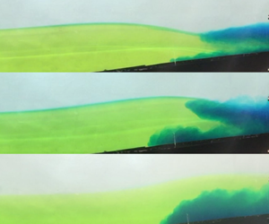
Figure 8. Progressive snapshots of a gravity current with  $Ri_{\unicode[STIX]{x1D70C}}=3.7$. Here, the interfacial intrusion generates a wave that propagates downstream well ahead of the intrusion or the underflow gravity current head.
In some instances, there is enough underflow and interflow such that we observe a significant interaction between the two. In figure 9(a) the underflow is seen propagating in the lower layer, but the crest of the internal wave is downstream of the gravity current head, characteristic of a launched wave. As the interflow enters the frame in figure 9(b), the position of the crest of the wave has surpassed that of the gravity current head, and the trough of the wave appears to be interacting with the gravity current head and causing it to flatten out. The height of the underflow in figure 9(b) is much smaller compared to the typical gravity current head in figure 9(a) with many billows entraining the ambient fluid. In figure 9(c), the trough of the wave has passed the front of the underflow, and is now generating an adverse pressure gradient that slows down the underflow. An indication of this retarded underflow speed is seen by comparing figures 9(c) and 9(d). The interflow, which propagates from right to left, appears to be moving faster than the front of the underflow, which has propagated significantly less. Maxworthy et al. (Reference Maxworthy, Leilich, Simpson and Meiburg2002) in experiments with horizontally propagating gravity currents in a linear stratification observed the same phenomenon, where the internal wave generated by the gravity current completely arrested the propagation of the head.

Figure 9. Progressive snapshots of a gravity current with  $Ri_{\unicode[STIX]{x1D70C}}=3.1$. Here, the launched wave from the interfacial intrusion arrests the motion of the underflow.
Figure 10 shows the gravity current internal wave Froude number  $Fr$ as a function of the gravity current Grashof number
  $Gr$. The uncertainty in the measurements arises from the imperfect tracking of the positions of the gravity current front and wave crest, and is a propagated 95 % confidence interval of the velocities. A low value of
  $Gr$ is suggestive of a weaker gravity current leading to an interflow-dominated situation, and a higher value of
  $Gr$ produces an underflow-dominated gravity current. For low
  $Gr$ cases, we find
  $Fr<1$, consistent with the expected interflow-dominated regime. As
  $Gr$ is increased,
  $Fr$ also increases, and the majority of the cases for intermediate
  $Gr$ have
  $Fr$ between 0.9 and 1. For the larger
  $Gr$ cases,
  $Fr$ appears to be greater than 1, because the gravity current speed is measured to be greater than the internal wave speed. However, this brings into question to which part of the gravity current the wave is responding. This question arises because of the highly vortical nature of the head of the gravity current, where the locked wave speed may be dictated by the speed of the billow-like structure in the lee of the gravity current head as opposed to the frontal speed of the head itself. The behaviour of the leading billow structure is highly transient and it appears to grow in size due to a continuous generation of baroclinic vorticity as well as a potential interaction between the pycnocline deflection caused by the billow and the billow itself, thus allowing it to grow. By measuring the propagation speed of the large billow structure behind the head and recalculating
  $Fr$, the values become
  $Fr\approx 1$ as expected for the locked cases. This result also suggests that there is a dispersive interaction between the head of the gravity current and the large billow-like structure behind the head, causing the two to separate from one another, a phenomenon that has not been observed in previous studies of gravity currents propagating in homogeneous environments.

Figure 10. Froude number of the generated wave as a function of the Grashof number of the gravity current. Circles show Froude numbers computed based on the gravity current frontal speed, and crosses show Froude numbers computed based on the velocity of the leading billow behind the head.
4 Discussion and conclusions
We used laboratory experiments to study the fate of negatively buoyant gravity currents propagating down an inclined slope into a quiescent two-layer ambient stratification. From vertical density profiles taken after the gravity current release, a typical gravity current was identified as having formed both underflow and interflow. Using hypothetical vertical density profiles as theoretical maximum and minimum cases for underflow and interflow, the partitioning of the current into underflow and interflow components was quantified using a non-dimensional centre of mass. By using a Richardson number defined as the ratio between density excess of the gravity current and the ambient stratification, a regime in which the splitting was a function of  $Ri_{\unicode[STIX]{x1D70C}}$ was identified, along with asymptotic behaviour in the splitting for the gravity currents tested.
Based on the final profiles as well as observations with tracer dye, gravity currents with low Richardson numbers that predominantly result in underflow were observed to also generate an interflow due to the transient interaction between the gravity current head and the pycnocline. The head of the gravity current vertically displaced the pycnocline, possibly creating an adverse pressure gradient for the tail portion of the gravity current and causing enhanced mixing to take place, leading to a following interflow. The consistent presence of an interflow is somewhat unexpected, and differs from the classical view of gravity currents in stratified media being either a pure underflow or interflow (Fischer et al. Reference Fischer, Koh, List, Koh, Imberger and Brooks1979).
Two different wave mechanisms were identified in the pycnocline response to the gravity current. In an underflow-dominated regime, the speed of the crest of the internal wave was locked to the speed of the head of the gravity current. For an interflow-dominated regime, the gravity current impinging on the pycnocline launched a wave that propagated faster than the gravity current head or interfacial intrusion. Using a Froude number comparing the speed of the gravity current to the phase speed of the wave, we characterized the launched and locked regimes. In gravity currents with the highest buoyancy flux and therefore Grashof number, we found that the internal wave was not in fact locked to the speed of the front of the gravity current but rather to the speed of the leading billow-like structure behind the head of the current.
A potential limitation to the generalization of the results presented regarding the quantification of the splitting of the gravity current is related to the shape of the vertical density and velocity profiles of the gravity current. Cortés et al. (Reference Cortés, Rueda and Wells2014b) measured both the density and velocity profiles of the gravity current and compared them to previous studies. Although trends were generally consistent for both subcritical and supercritical gravity currents, there were differences in the shapes of the gravity current profiles, and Cortés et al. (Reference Cortés, Rueda and Wells2014b) showed that this would have an impact on the splitting behaviour of the gravity current. Currently there is no unifying theory or dimensionless parameter to describe the structure of the density and velocity profiles of a gravity current, which would ultimately lead to a more generalized parameterization of its splitting. While the splitting transitional  $Ri_{\unicode[STIX]{x1D70C}}$ and resulting
  $M_{c}^{\ast }$ may vary due to varying shapes of the velocity and density profiles, there are two more generalizable results emerging from our work that should apply to stratified water bodies in general. First, we can expect that a dense gravity current in a stratified system will undergo some degree of splitting, and exhibit both underflow and interflow characteristics compared to the more traditional thinking of gravity currents being purely underflow or purely interflow. Second, upon reaching the pycnocline, the underflow portion of the gravity current will produce a locked wave at the interface, while the interflow part will produce a launched wave at the interface.
Acknowledgements
We gratefully acknowledge assistance in the laboratory from L. Clark, and for the fabrication of the experimental apparatus by B. Sabala. This work was supported by National Science Foundation grant no. OCE 1634389. We are also grateful to three anonymous reviewers for their thoughtful critique of the manuscript.
Declaration of interests
The authors report no conflict of interest.


