2.1 Velocity measurements

Hot-wire anemometry was used for point measurements of velocities, especially at the nozzle exit. To compute the power spectral density (PSD), 30 blocks of 8192 samples were recorded with a low-pass filter at 3 kHz and acquisition frequency of 9 kHz, using a Dantec P11 single-wire probe (1.25 mm long and $5~\unicode[STIX]{x03BC}\text{m}$ diameter sensor).

For the HS-SPIV, two Phantom V710 high-speed cameras equipped with 105 mm lenses at an $f_{\#}=8$ aperture were used in forward scattering configuration. A high-repetition-rate double-pulse Nd:YLF 527 nm laser synchronized with the cameras generated a 2.5 mm thick light sheet. The inter-pulse time was adjusted such that a maximum displacement of 7 pixels is obtained on the camera images. Sixteen blocks of 4096 double-frame image pairs were recorded at an acquisition frequency $F_{a}=2.5~\text{kHz}$. Velocity vectors were computed using FOLKI-SPIV, an in-house PIV software described in Champagnat et al. (Reference Champagnat, Plyer, Le Besnerais, Leclaire, Davoust and Le Sant2011). An interrogation window size of 31 pixels was chosen, which yielded a spatial resolution of the vector field of 2.7 mm ($0.018D$). All the HS-SPIV measurements presented here were made in the $Z=2D$ cross-sectional plane. Figure 3(b) summarizes this through a schematic representation of the set-up. The $Z=2D$ plane was chosen as being sufficiently downstream such that the mixing layer is fully developed and has lesser influence of the upstream conditions, including exiting boundary layer characteristics and that of the jet facility. Additionally, it was upstream enough to allow the study of the initial evolution of the structures and also such that the required measurement plane could be captured by the available HS-PIV system to obtain a good spatial resolution.

To provide an estimate of the uncertainty associated with the quantities of interest obtained with HS-SPIV in this study, we monitored the distribution of values obtained in flow zones in which these quantities were known from physics to be uniform. We then chose the associated uncertainty estimate as $\pm 2\unicode[STIX]{x1D70E}$ of the distribution, $\unicode[STIX]{x1D70E}$ standing for the standard deviation (leading to a 95 % confidence level if the distribution were Gaussian). The uncertainty on the mean axial velocity was then found to be ±0. 3 %, and on the turbulence intensities to be ±0. 4 % of $U_{j}$. For the root mean square (r.m.s.) of the vorticity field, an uncertainty of ±6. 0 % was estimated. Note that the uncertainties estimated in such a way thus account for measurement noise (in the case of averaged fluctuating quantities) as well as possible residual bias sources of HS-SPIV, such as peak locking. Statistical error is found to be negligible, this point having been verified through a convergence study. It should be noted that, given the approach chosen, these estimates, however, cannot account for the effect of spatial filtering due to the presence of significant flow gradients at the scale of the PIV interrogation windows. However, we will provide a typical estimate of this phenomenon by comparing HS-SPIV and HWA results, in § 3.1.

2.2 Axisymmetric excitation and parameters studied

Acoustic excitation was achieved by means of a loudspeaker mounted on top of the settling chamber, which provided axisymmetric forcing at the nozzle exit. The loudspeaker was driven by a pure sine wave whose amplitude can be varied through the voltage supplied to the loudspeaker. Irrespective of the exit jet velocities $U_{j}$, significant amplitudes of excitation were obtained at a frequency $F$ of 52 Hz, which has thus been assumed to be one of the resonant frequencies of the settling chamber. Our first aim is to selectively excite the most energetic $m=0$ mode to demonstrate the validity of the hypothesis of Davoust et al. (Reference Davoust, Jacquin and Leclaire2012), which accounts for the radial organization of streamwise vortices found in high-$Re$ jets. Figure 4 shows the axial velocity spectra at $Z=2D$ for a range of $U_{j}$. The peak in the spectra scales with $U_{j}$ to yield a constant Strouhal number of $St=FD/U_{j}\approx 0.49$. As the excitation frequency $F_{e}$ in our experiments had to be fixed at 52 Hz in order to reach sufficient amplitudes, we chose to set the jet exit velocity to $U_{j}=15.9~\text{m}~\text{s}^{-1}$. This resulted in a Reynolds number $Re=1.5\times 10^{5}$ and excitation Strouhal number, $St_{e}=F_{e}D/U_{j}=0.49$.

We then varied the $Re$ of the flow, by changing $U_{j}$, to determine the robustness of the proposed mechanism for different flow parameters. In that process, it was noted that transitional and fully turbulent boundary layers were obtained with the same strip, depending on the exit velocity. The state of the boundary layer is determined here according to the classification of Zaman (Reference Zaman1985), based on the mean velocity profile and the peak turbulence intensities in the exiting boundary layer. For instance, the $Re=1.5\times 10^{5}$ jet has an initially transitional (or more precisely nominally laminar) boundary layer that is neither fully laminar nor fully turbulent, as quite often encountered in applications, this point having been investigated in particular by Zaman (Reference Zaman2012) with regards to jet noise. However, it will be shown here that, interestingly, this boundary layer state has no observable influence on the dynamics under consideration.

The influence of $St_{e}$ on the discussed interaction between the $m=0$ mode and streamwise vortices was also explored. This was achieved by varying $U_{j}$ at the fixed frequency of excitation, 52 Hz, in order to maintain the possibility of reaching high excitation amplitudes. Table 1 gathers the explored values, along with the corresponding $St_{e}$ and boundary layer states. Note that, for one of the exit velocities, we also removed the carborundum strip in order to reach laminar boundary layer conditions. Four values of $U_{j}$ were examined, $U_{j}=9.5~\text{m}~\text{s}^{-1}$ being the lowest possible one in the current set-up and the highest being $U_{j}=34.9~\text{m}~\text{s}^{-1}$. The $U_{j}=9.5~\text{m}~\text{s}^{-1}$ jet was in fact not excited, as it resulted in amplification of different frequencies at the nozzle exit. We ascribe this to an operational instability of the centrifugal fan upstream of the loudspeaker at low velocities. This point was thus considered within the $Re$ variation only. The other three values for $U_{j}$ were chosen to target $St_{e}=0.49$, 0.35 and 0.22. The value $St_{e}=0.35$ was chosen to be in the range of the so-called preferred mode of jets (Crow & Champagne Reference Crow and Champagne1971) and $St_{e}=0.22$ to be in the lower end of the natural spectrum of figure 4, which corresponds to a less energetic $m=0$ mode.

Figure 4. Power spectral density (PSD) of the non-dimensional axial velocity fluctuations ($u_{z}^{\prime }/U_{j}$) measured on the jet axis at $Z=2D$, as a function of $St=fD/U_{j}$ for the exit jet velocities $U_{j}=15.8~\text{m}~\text{s}^{-1}$ (dashed line), $22.2~\text{m}~\text{s}^{-1}$ (dash-dotted line) and $28.0~\text{m}~\text{s}^{-1}$ (dotted line).

Table 1. Parameters explored in this study. Note that the most energetic frequency at $Z=2D$ scales with $U_{j}$ to give $St\approx 0.49$, and that the excitation frequency was fixed at 52 Hz.

2.3 Frame of reference and notation

The acquired HS-SPIV data are transformed from Cartesian ($x,y$) to cylindrical ($r,\unicode[STIX]{x1D703}$) coordinates using bilinear interpolation, with a resolution of $N_{r}=34$ points in the radial and $N_{\unicode[STIX]{x1D703}}=128$ points in the azimuthal directions. This preserves the resolution in the shear layer on both the grids. The mean velocity is subtracted from the instantaneous field to yield the fluctuation velocity field, which is the basis for all the statistical measures presented in this paper.

In the following sections, we represent dimensional quantities by uppercase ($R,\unicode[STIX]{x1D6E9},Z$) and non-dimensional by lowercase ($r,\unicode[STIX]{x1D703},z$) symbols in the cylindrical coordinate system. Lengths and velocities are presented in non-dimensional forms scaled with the nozzle exit diameter ($D$) and centreline average jet velocity ($U_{j}$), respectively. Non-dimensional time is expressed by $t$ and frequency by Strouhal number, $St=FD/U_{j}$, with $St_{e}$ denoting the excitation Strouhal number, as already introduced above. We denote the components of the mean velocity vector by ($u_{r},u_{\unicode[STIX]{x1D703}},u_{z}$), the fluctuations by a prime ($u_{r}^{\prime },u_{\unicode[STIX]{x1D703}}^{\prime },u_{z}^{\prime }$) and the turbulence or fluctuation intensities by superscript $rms$, denoting root mean square (e.g. $u_{z}^{rms}=\langle u_{z}^{\prime }\rangle ^{1/2}$). Unless specified, most of the measurements are at $z=2$, a cross-sectional plane at two diameters from the nozzle exit.

2.4 Spectral proper orthogonal decomposition

We have used SPOD to extract the most energetic structures in the flow, similar to Davoust et al. (Reference Davoust, Jacquin and Leclaire2012). Owing to the statistical stationarity and axisymmetry of the flow, the SPOD eigenfunctions in time and azimuthal direction are then the Fourier modes. In practice, each component ($u_{i}$ for $i=z,r,\unicode[STIX]{x1D703}$) of the fluctuations of the velocity vector are first Fourier-transformed in $t$ and $\unicode[STIX]{x1D703}$ as

(2.1)$$\begin{eqnarray}\hat{u} _{i}(r,m,f)=\int _{0}^{t_{0}}\int _{0}^{2\unicode[STIX]{x03C0}}u_{i}^{\prime }(r,\unicode[STIX]{x1D703},t)\text{e}^{-\text{i}(m\unicode[STIX]{x1D703}+2\unicode[STIX]{x03C0}ft)}\,\text{d}\unicode[STIX]{x1D703}\,\text{d}t,\end{eqnarray}$$

where $t_{0}$ is the acquisition length of each block, and $f$ is a duplicate notation for the reduced frequency or Strouhal number $St$, which we use here instead of $St$ to avoid confusion in the equations. SPOD modes $\unicode[STIX]{x1D719}_{i}^{(n)}(r,m,f)$ with $n=1,2,\ldots$ for the given ensemble are found using

(2.2)$$\begin{eqnarray}\int _{0}^{r_{0}}B_{ij}(r,r^{\prime },m,f)\unicode[STIX]{x1D719}_{j}^{(n)}(r^{\prime },m,f)\,\text{d}r^{\prime }=\unicode[STIX]{x1D706}^{(n)}(m,f)\unicode[STIX]{x1D719}_{i}^{(n)}(r,m,f),\end{eqnarray}$$

where $r_{0}$ is the radial extent of the measurement plane and $\unicode[STIX]{x1D706}^{(n)}$ are the eigenvalues. The Hermitian symmetric kernel ($B_{ij}$) is the weighted two-point cross-spectrum given by

(2.3)$$\begin{eqnarray}B_{ij}(r,r^{\prime },m,f)=r^{1/2}\langle \hat{u} _{i}(r,m,f)\hat{u} _{j}^{\ast }(r^{\prime },m,f)\rangle {r^{\prime }}^{1/2},\end{eqnarray}$$

with $x^{\ast }$ representing the complex conjugate of $x$. The angle bracket $\langle ~\rangle$ denotes the ensemble average over all the data blocks. The members of the ensemble can be reconstructed through

(2.4)$$\begin{eqnarray}\hat{u} _{i}(r,m,f)=\frac{1}{r^{1/2}}\mathop{\sum }_{n}\hat{a}^{(n)}(m,f)\unicode[STIX]{x1D719}_{i}^{(n)}(r,m,f),\end{eqnarray}$$

where $\hat{a}^{(n)}(m,f)$ are the coefficients found by projecting the velocity vector onto the SPOD basis as

(2.5)$$\begin{eqnarray}\hat{a}^{(n)}(m,f)=\int _{0}^{r_{0}}r^{1/2}\hat{u} _{i}(r,m,f)\unicode[STIX]{x1D719}_{i}^{\ast (n)}(r,m,f)\,\text{d}r.\end{eqnarray}$$

More details about the implementation of SPOD are given in appendix A.

3.1 Inflow conditions and characterization of HS-SPIV measurements with HWA

Mean and fluctuation intensity profiles of the axial velocity near the nozzle exit, at $z=0.003$, are shown in figure 5. The exiting boundary layer is transitional. While the mean velocity fits the Blasius boundary layer profile, the peak turbulence intensity is as high as 2 % for the boundary layer to be fully laminar. The boundary layer momentum thickness, $\unicode[STIX]{x1D6FF}_{\unicode[STIX]{x1D703}}$, is equal to 0.0021. It is known that the inflow conditions of the exiting boundary layer from the nozzle can play a role in the downstream evolution of jets (Hussain & Zedan Reference Hussain and Zedan1978; Bogey & Bailly Reference Bogey and Bailly2010). However, it will be shown in § 5.1 that the phenomenon observed in the current work is not sensitive to these conditions.

With regards to temporal aliasing due to the high acquisition rate of 2.5 kHz for HS-SPIV, it has been shown in Davoust et al. (Reference Davoust, Jacquin and Leclaire2012) that the limited spatial resolution of HS-SPIV also prevents temporal aliasing. Figure 6(a) shows this temporal filtering through the comparison of frequency spectra of axial velocity fluctuations at $z=2$ obtained with HS-SPIV and HWA. The two techniques agree well up to $St=1$, after which HS-SPIV has a cutoff of up to -8 dB (at $St=9.5$) in the shear layer. Besides, it can be noted that the shear layer exhibits a broadband spectra, while in the core there is a broad peak, as in figure 4, which can be interpreted as a signature there of the large-scale structures from the shear layer. Also, the mean and fluctuation intensities at $z=2$ are compared for the two techniques in figure 6(b). Good agreement is found in the core, whereas in the shear layer, HS-SPIV captures up to 80 % of the fluctuations owing to its inherent filtering of turbulence.

Figure 5. Axial velocity profiles of the unexcited jet at $Re=1.5\times 10^{5}$ near the nozzle exit ($z=0.003$) obtained using HWA: mean velocity (—●—) and r.m.s. (—$\times$—).

Figure 6. Comparison between HS-SPIV and HWA measurements for the unexcited jet at $Re=1.5\times 10^{5}$ at $z=2$. (a) PSD of the axial velocity in the jet core ($r=0.24$) and shear layer ($r=0.51$): solid black line, HS-SPIV; and dotted blue line, HWA measurements. (b) Radial profiles of mean and r.m.s. of the axial velocity: solid black line, HS-SPIV; and dashed blue lines, HWA measurements, for $u_{z}|_{z=2}$ (– –●– –) and for $u_{z}^{rms}|_{z=2}$ (– –$\times$– –).

3.2 Azimuthal and frequency distribution

We then look at the distribution of velocity fluctuations with respect to frequency $f$ and azimuthal wavenumber $m$, along with the contribution from the most energetic structures (corresponding to $n=1$, i.e. the first POD mode) at $z=2$. Here we restrict to the main observations, as the natural dynamics of the present jet at $Re=1.5\times 10^{5}$ were found to be nearly identical to those of Davoust et al. (Reference Davoust, Jacquin and Leclaire2012) at $Re=2.1\times 10^{5}$. Using the same notation as in that study, the azimuthal and frequency spectra can be computed from (2.3). The unweighted two-point cross-spectrum $S_{ij}$ is given by

(3.1)$$\begin{eqnarray}S_{ij}(r,r^{\prime },m,f)=\langle \hat{u} _{i}(r,m,f)\hat{u} _{j}^{\ast }(r^{\prime },m,f)\rangle =\frac{B_{ij}(r,r^{\prime },m,f)}{r^{1/2}{r^{\prime }}^{1/2}}.\end{eqnarray}$$

The azimuthal spectrum $Sm_{i}(r,m)$, which represents the fraction of the kinetic energy contained in the $i$th component of the fluctuating velocity vector corresponding to mode $m$ at radius $r$, can be computed as

(3.2)$$\begin{eqnarray}Sm_{i}(r,m)=\int S_{ii}(r,r,m,f)\,\text{d}\,f=\frac{1}{r}\int B_{ii}(r,r,m,f)\,\text{d}\,f.\end{eqnarray}$$

Truncating to $n=1$ POD mode, the azimuthal spectrum can be expressed in terms of the eigenfunctions $\unicode[STIX]{x1D719}_{i}$ as

(3.3)$$\begin{eqnarray}Sm_{i}^{(1)}(r,m)=\frac{1}{r}\int \unicode[STIX]{x1D706}^{(1)}(m,f)|\unicode[STIX]{x1D719}_{i}^{(1)}(r,m,f)|^{2}\,\text{d}\,f.\end{eqnarray}$$

Figure 7 shows the azimuthal spectra of the axial velocity, $Sm_{z}(r,m)$, at two radial locations, in the jet core and the shear layer. The dominance of the $m=0$ mode in the core ($r=0.24$) and of the higher azimuthal modes ($m=4{-}7$) in the shear layer ($r=0.51$) can be seen, in agreement with previous studies (Citriniti & George Reference Citriniti and George2000; Jung et al. Reference Jung, Gamard and George2004). It was shown in Davoust et al. (Reference Davoust, Jacquin and Leclaire2012) that the second most energetic azimuthal mode in the jet core, the $m=\pm 1$ mode, is related to the tilting of the vortex rings with respect to the jet axis, as was also observed by Liepmann & Gharib (Reference Liepmann and Gharib1992) in their visualizations. It is interesting to look at the dominance of higher azimuthal modes in the shear layer. Azimuthal wavenumbers in the neighbourhood of $m=5$ have the maximum energy fraction, as also found in past experimental studies (see e.g. the SPOD results of Glauser et al. (Reference Glauser, Leib and George1987), Citriniti & George (Reference Citriniti and George2000) and Jung et al. (Reference Jung, Gamard and George2004)), and therefore have been often used in numerical simulations to trigger three-dimensional instabilities in jets (Martin & Meiburg Reference Martin and Meiburg1991; Brancher, Chomaz & Huerre Reference Brancher, Chomaz and Huerre1994). Figure 7 includes as well the truncated system with only the $n=1$ POD mode, where it can be seen that the first POD mode approximates well the dynamics in the jet core. However, in the shear layer, a higher number of POD modes are required to capture the turbulent flow region, with still a significant contribution from the $n=1$ POD mode.

Figure 7. Azimuthal spectra of the axial velocity corresponding to full spectra $Sm_{z}(r,m)$ (●) and to the first POD mode only, $Sm_{z}^{(1)}(m)$ (

): (a) in the core, $r=0.24$; and (b) in the shear layer, $r=0.51$.

The frequency spectrum $Sf_{i}(r,f)$ can be computed as

(3.4)$$\begin{eqnarray}Sf_{i}(r,f)=\mathop{\sum }_{m}S_{ii}(r,r,m,f).\end{eqnarray}$$

Again, on truncation to $n=1$ POD mode, it can be expressed as

(3.5)$$\begin{eqnarray}Sf_{i}^{(1)}(r,f)=\frac{1}{r}\mathop{\sum }_{m}\unicode[STIX]{x1D706}^{(1)}(m,f)|\unicode[STIX]{x1D719}_{i}^{(1)}(r,m,f)|^{2}.\end{eqnarray}$$

The frequency spectrum of the axial velocity in the jet core (figure 8) also shows the significant contribution of the $m=0$ and $n=1$ POD mode to the overall dynamics in the core. With the inclusion of the first azimuthal modes ($m=\pm 1$), the truncated system containing just the $n=1$ POD mode again provides a good description of the dynamics. The broad peak in the spectrum arises from the $m=0$ mode, which is spread over a range of frequencies, with the most energetic frequency occurring at $St=0.49$. This peak can be interpreted as the passage frequency of the most energetic vortex rings at $z=2$. Axisymmetric excitation at this frequency will be studied in the following section.

Figure 8. Frequency spectra of the axial velocity at $z=2$ in the core at $r=0.24$; the full spectrum $Sf_{i}(r,f)$ is represented by the solid black line. The contribution from the first POD mode, $Sf_{i}^{(1)}(r,f)$, corresponding to $m=0$ is denoted by the blue dashed line, $m=\pm 1$ by the red and green dotted lines and $m=[-1,0,1]$ by the blue solid line with filled circles, presented on a linear scale.

4.1 Fluctuation intensities

Figure 10 shows the effect of increasing excitation amplitude on the exiting boundary layer, measured in terms of axial velocity. While no appreciable change is observed in the mean profile even at the highest amplitude (4.8 %), there is a monotonic increase in the r.m.s. velocities in the jet core as well as in the shear layer. The peak r.m.s. values reach up to 12 % for the most excited case, while the mean profiles remain of the Blasius type, thus making the boundary layer transitional whatever the excitation level.

Figure 10. The effect of excitation on the exit boundary layer ($z=0.003$) in terms of axial velocity measured by HWA: (a) mean and (b) fluctuation intensities, where the solid black line represents the unexcited jet, and other lines represent excitation at $u_{z}^{rms}=1.4\,\%$ (dotted red line), at 2.6 % (dash-dotted green line) and at 4.8 % (dashed blue line).

The radial profiles of fluctuation intensities at $z=2$ are shown in figure 11, averaged in the azimuthal direction, as the flow is statistically axisymmetric. With increasing excitation amplitudes, one observes an increase in the r.m.s. of axial and radial components of velocity, which are mainly induced by the vortex rings, with no appreciable change in the azimuthal component, as expected. In figure 11(a) $u_{z}^{rms}$ can be seen to develop a local minimum at $r\approx 0.58$, not observed in the natural case. The phase-averaged longitudinal views of streamwise vorticity and azimuthal vorticity shown in figure 12, performed on a Taylor reconstruction and using the excitation as reference signal, indicate that this location of the minimum coincides with the core of the vortex rings. Details about the use of Taylor’s hypothesis are given in § 4.2, and about the phase averaging in appendix B. The appearance of this minimum in $u_{z}^{rms}$ could thus be due to the regularization in the formation of vortex rings at the excitation frequency, i.e. the cores of the rings could occur at the same radial location in the shear layer as they convect downstream. When considering the azimuthal spectra of the axial velocity in the shear layer at $r=0.51$ (figure 13b), one observes a decrease in the higher azimuthal modes with increasing levels of excitation. This again suggests the increasing axisymmetry of the flow with excitation, even in the shear layer. On the other hand, no appreciable change in the distribution of higher azimuthal modes is observed in the jet core at $r=0.24$ in figure 13(a), except for slight elevations in their energy levels.

Going back to the phase-averaged vorticity fields of figure 12, we see a remarkable persistence of the vortical structures even upon phase averaging. This compares well with the classical portrait observed in the visualizations of Liepmann & Gharib (Reference Liepmann and Gharib1992) for round jets at low $Re$, where the streamwise vortices were found wrapping around the azimuthal rings. Also, regions of high positive azimuthal vorticity fluctuations contain high streamwise vorticity fluctuations (see the light patches close to $r\approx 0.6$), suggesting that the rings are corrugated in the azimuthal direction and not perfectly axisymmetric, as could have been expected with the excitation. Possibly, the peak observed at $r=0.58$ in the r.m.s. profile of $\unicode[STIX]{x1D714}_{z}^{\prime }$ in figure 11(d) could also be a trace of this corrugation. However, it must be noted that there should be a contribution from $\unicode[STIX]{x1D714}_{z}^{\prime }$ in the streamwise vortices as well towards this peak value. The other peak in the r.m.s. profile occurs at $r=0.38$, which is near the downstream edge of a streamwise vortex. The streamwise vortices appear closest to the vortex rings at this location and near the upstream edge, where they wrap around the rings. Besides, the $\unicode[STIX]{x1D714}_{z}^{rms}$ values remain almost the same with increasing levels of excitation and the radial extent where they are significant increases, indicating the spread of streamwise vorticity into the jet core. Section 4.3 will shed more light into this, where we will study the streamwise vorticity organization in detail.

Figure 11. Radial profiles of fluctuation intensities at $z=2$ of (a) axial, (b) radial and (c) azimuthal velocity and (d) streamwise vorticity, where the solid black line represents the unexcited jet, and other lines represent excitation at $u_{z}^{rms}=1.4\,\%$ (dotted red line), at 2.6 % (dash-dotted green line) and at 4.8 % (dashed blue line).

The azimuthal spectra of $\unicode[STIX]{x1D714}_{z}^{\prime }$ are presented in figure 14. For the unexcited jet, the streamwise vorticity is distributed over a range of azimuthal wavenumbers from $m=2$ to 10, while for the most excited case, that range is narrowed down to $m=5{-}9$ at $r=0.38$, and around $m=5$ at $r=0.58$. This suggests that excitation also leads to a regularization in the formation of streamwise vortices. A look into the azimuthal spectra of $u_{r}^{\prime }$ and $u_{\unicode[STIX]{x1D703}}^{\prime }$, from which $\unicode[STIX]{x1D714}_{z}^{\prime }$ is computed, reveals that the two peaks at $r=0.38$ and 0.58 stem from the distribution of the azimuthal velocity component. Noting that $u_{\unicode[STIX]{x1D703}}^{\prime }$ can be induced by the streamwise vortices but not by the $m=0$ mode, the azimuthal wavenumber in figure 14 at $r=0.38$ could thus possibly be interpreted as the average number of streamwise vortices in the shear layer. The azimuthal wavenumber at $r=0.58$, pertaining to the vortex rings as mentioned above, could relate to the number of corrugations that they exhibit, the $u_{\unicode[STIX]{x1D703}}^{\prime }$ being induced by the tilted part of the rings in the axial direction. Owing to the closeness of the maximal values for $m$ at those two radial locations, it could be hypothesized that the presence of the streamwise vortices and the corrugations in the vortex rings could be linked to one another. Indeed, Martin & Meiburg (Reference Martin and Meiburg1991) found in round jets that the streamwise vortices caused waviness on the cores of the vortex rings where they wrapped around the rings, and Lasheras & Choi (Reference Lasheras and Choi1988) observed wavy undulations in the spanwise rollers caused by streamwise vortices in planar mixing layers.

4.2 Taylor’s reconstruction in the axial direction

Since in our experiments, the HS-SPIV measurement plane is at a fixed downstream location, the local spatial structure of the flow in the axial direction is derived from the temporal snapshots using Taylor’s hypothesis. For low turbulence intensities compared to the mean flow speed, Taylor’s hypothesis of frozen turbulence allows one to view temporal fluctuations at a fixed point in space as a result of a frozen spatial structure convecting past that point at the mean flow speed, or the convection velocity $u_{c}$ (Taylor Reference Taylor1938). An appropriate convection velocity and the validity of the hypothesis must be carefully considered while applying this hypothesis. Davoust & Jacquin (Reference Davoust and Jacquin2011) proposed a method based on the continuity equation to calculate $u_{c}$, particularly suited for experimental data. Computing in the Fourier space, $u_{c}$ was obtained as a function of frequency and spatial location in a measurement plane normal to the mean flow. The application of this method to compute $u_{c}$ in the current work is detailed in appendix C.

Figure 12. Phase-averaged (a) $\unicode[STIX]{x1D714}_{z}^{\prime }$ and (b) $\unicode[STIX]{x1D714}_{\unicode[STIX]{x1D703}}^{\prime }$ for two periods, reconstructed using Taylor’s hypothesis from HS-SPIV measurements at $z=2$, for the most excited case at 4.8 %. Extraction in the longitudinal plane. See § 4.2 for more details on Taylor’s reconstruction.

Figure 13. Variation of azimuthal spectra of the axial velocity with increasing excitation levels, where the solid black line represents the unexcited jet, and the other lines represent excitation at $u_{z}^{rms}=1.4\,\%$ (dotted red line), at 2.6 % (dash-dotted green line) and at 4.8 % (dashed blue line). This is a close-up of the higher azimuthal modes, the $m=0$ mode having very high amplitudes for the excited cases (a) in the core $r=0.24$ and (b) in the shear layer $r=0.51$.

Figure 14. Azimuthal spectra of the streamwise vorticity ($\unicode[STIX]{x1D714}_{z}^{\prime }$) for the (a) unexcited jet and (b) excited jet at 4.8 %.

We can derive physical intuition for the flow and the effect of excitation through such a reconstruction, as shown in figure 15 for a natural jet and its excited counterpart at an excitation level of $u_{z}^{rms}|_{z=0}=4.8\,\%$. The axial coordinate is $z=-u_{c}t$. As expected, excitation is seen to raise the inherent order in the turbulent flow above the background noise. Also, in the excited case one can discern the classical structure of the near field of a jet through excitation, which consists of a periodic array of vortex rings and counter-rotating streamwise vortices, organized in the azimuthal direction (Liepmann & Gharib Reference Liepmann and Gharib1992). The wrapping of the streamwise vortices around the rings and wave-like undulations on the ring cores are evident in the excited jet. Similar observations of core undulations were made by Lasheras & Choi (Reference Lasheras and Choi1988), for plane free shear layers subjected to sinusoidal perturbations. Also, the inclination of the streamwise vortices is towards the jet centreline near the upstream region of the rings, while immediately downstream, it can be observed to be away from the centreline. In the unexcited jet, on the other hand, they tend to be more aligned in the axial direction, though it is rather difficult to comment clearly on the structures in there. For the jet excited at 4.8 %, we could count the approximate number of streamwise vortices from the Taylor’s reconstruction to be around 16, eight of each sign, thus corresponding to an azimuthal wavenumber $m=8$. This lies in the range of dominant azimuthal wavenumbers of $\unicode[STIX]{x1D714}_{z}^{\prime }$ seen in figure 13 at $r=0.51$, thus supporting the inference made in the previous section that those azimuthal wavenumbers could possibly indicate the number of streamwise vortices.

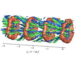
Figure 15. Taylor’s reconstruction of vorticity fluctuations in the axial direction ($z_{c}=-u_{c}t$) for (a) the natural jet and (b) the excited jet at $u_{z}^{rms}|_{z=0}=4.8\,\%$. The orange colour corresponds to isosurfaces of $\unicode[STIX]{x1D714}_{\unicode[STIX]{x1D703}}^{\prime }=+3$, the green and blue to those of $\unicode[STIX]{x1D714}_{z}^{\prime }=+3$ and $\unicode[STIX]{x1D714}_{z}^{\prime }=-3$, respectively. The flow is from left to right.

4.3 Streamwise vorticity organization

In order to visualize the organization of streamwise vorticity fluctuations in our flow, we compute the following autocorrelation, similar to Davoust et al. (Reference Davoust, Jacquin and Leclaire2012):

(4.1)$$\begin{eqnarray}C_{\unicode[STIX]{x1D714}_{z}\unicode[STIX]{x1D714}_{z}}(r,r^{\prime },\unicode[STIX]{x1D703}^{\prime },t^{\prime })=\frac{\langle \unicode[STIX]{x1D714}_{z}^{\prime }(r,\unicode[STIX]{x1D703},t)\unicode[STIX]{x1D714}_{z}^{\prime }(r^{\prime },\unicode[STIX]{x1D703}+\unicode[STIX]{x1D703}^{\prime },t+t^{\prime })\rangle _{\unicode[STIX]{x1D703}}}{\langle {\unicode[STIX]{x1D714}_{z}^{\prime }}^{2}(r,\unicode[STIX]{x1D703},t)\rangle _{\unicode[STIX]{x1D703}}^{1/2}\langle {\unicode[STIX]{x1D714}_{z}^{\prime }}^{2}(r^{\prime },\unicode[STIX]{x1D703},t)\rangle _{\unicode[STIX]{x1D703}}^{1/2}}.\end{eqnarray}$$

Here $\langle ~\rangle _{\unicode[STIX]{x1D703}}$ denotes an average over both data blocks and $\unicode[STIX]{x1D703}$, as the flow has statistical stationarity and azimuthal homogeneity. Contours of $C_{\unicode[STIX]{x1D714}_{z}\unicode[STIX]{x1D714}_{z}}$ for $t^{\prime }=0$, i.e. correlation of $\unicode[STIX]{x1D714}_{z}^{\prime }$ at a particular instant of time in the cross-section averaged over all snapshots, would give a probable vortex structure in a statistical sense. Figures 16 and 17 show these contours in the cross-sectional plane at $z=2$, and in the longitudinal plane reconstructed using Taylor’s hypothesis, respectively, at three radial locations in the jet. The plots containing the contours are accompanied by schematics depicting the correlation process at the top. These positions, $r=0.38$, 0.51 and 0.68, were chosen to represent the downstream, middle and upstream part of a streamwise vortex (see e.g. figure 12).

Figures 16 and 17 compare the streamwise vorticity organizations found for the natural jet (left column), and for the excited jet at $u_{z}^{rms}|_{z=0}=2.6\,\%$ (right column). In the left column (i) of figure 16, we can see patches of negative correlation above and below the probing point at $r=0.51$, located near the centre of the shear layer, indicating the presence of opposite-signed vorticity in the radial direction. This, along with the correlation patches at other radial probing points, suggests a radial organization of streamwise vortices, as was also observed by Davoust et al. (Reference Davoust, Jacquin and Leclaire2012) at $Re=2.1\times 10^{5}$. In the right column (ii) of figure 16, we observe an azimuthal organization of the streamwise vortices, especially at $r=0.38$, where the negative patches on the left and the right are of larger amplitude than the patch on top, and also at $r=0.51$, where negative patches on all sides have the same amplitude, the patch on top being located farther away. Consistently, this azimuthal organization is also apparent in the Taylor reconstructions of figure 15. The strength of this azimuthal correlation, however, tends to decrease as we move away from the jet centreline, becoming nearly equal to the radial correlation. To us, this trend cannot be explained with the present figures, and will require considering correlations separately in the braid and ring regions. This will be performed below while presenting the most excited case, $u_{z}^{rms}|_{z=0}=4.8\,\%$, where the effects of maximum excitation allow a clearer analysis of the vortical organization.

Figure 16. A typical organization of streamwise vorticity in the cross-sectional plane at $z=2$, evidenced through isocontours of $C_{\unicode[STIX]{x1D714}_{z}\unicode[STIX]{x1D714}_{z}}(r,r^{\prime },\unicode[STIX]{x1D703}^{\prime },t^{\prime }=0)$ at three radial locations in the jet. On the top, (ai) is a schematic depicting the correlation process. Columns (b–d) correspond to the natural (i) and excited (ii) cases, exhibiting radial and azimuthal organizations, respectively. Excitation is performed at $St_{e}=0.49$, $u_{z}^{rms}|_{z=0}=2.6\,\%$. Solid lines represent positive correlation while dashed lines represent negative correlation.

Figure 17. Similar organization of streamwise vorticity as in figure 16 but in a longitudinal plane reconstructed using Taylor’s hypothesis: (ai) schematic depicting the correlation process, columns (b–d) isocontours of $C_{\unicode[STIX]{x1D714}_{z}\unicode[STIX]{x1D714}_{z}}(r,r^{\prime },\unicode[STIX]{x1D703}^{\prime }=0,t^{\prime })$ at the indicated radial locations. Columns correspond to the natural (i) and excited (ii) cases, exhibiting radial and azimuthal organizations, respectively.

A similar image unfolds when we look at the longitudinal planes in figure 17. The left column (i) shows negative correlation patches aligned along the positive patch around the probing point, again giving a global portrait of radially organized streamwise vortices. The correlations appear to be elongated and inclined to the jet axis. The angle of inclination to the jet centreline is seen to increase as we probe away from the centreline, as was noted in Davoust et al. (Reference Davoust, Jacquin and Leclaire2012). In the column on the right (ii), these negative patches are reduced, indicating the quasi-absence of opposite-signed vortices in the radial direction. Interestingly, at $r=0.38$ we still see some correlation in the radial direction, with the maximum negative correlation of -0. 07 around $r=0.58$. This will also be discussed in more detail when analysing the most excited case, at $u_{z}^{rms}|_{z=0}=4.8\,\%$.

Seeing these differences in the organization of streamwise vortices between a natural and an excited jet, questions arise naturally as to the amplitude of excitation necessary for the change to occur, as well as its sudden or progressive character. To shed light on this, we now describe a case with intermediate excitation compared to the previous one, i.e. $u_{z}^{rms}|_{z=0}=1.4\,\%$, represented in figure 18. In this figure, one sees the presence of negative lobes of $C_{\unicode[STIX]{x1D714}_{z}\unicode[STIX]{x1D714}_{z}}$ of significant magnitude in both radial and azimuthal directions, which leads us to term this organization as ‘transitional’. In practice, when considering other intermediate levels, one observes that the switch of organization, from radial in the natural case, to azimuthal in sufficiently excited cases, is not sudden but progressive, via these transitional states, with obviously azimuthal organizations appearing from $u_{z}^{rms}|_{z=0}=2.6\,\%$.

We now turn to the vortical organization obtained for the highest level of excitation that could be reached in this study, i.e. $u_{z}^{rms}|_{z=0}=4.8\,\%$, plotted in figure 19. This figure contains slightly different and additional information compared to the previous ones, in order to explain most precisely the typical correlation organizations observed in the excited cases. In addition to correlations $C_{\unicode[STIX]{x1D714}_{z}\unicode[STIX]{x1D714}_{z}}$ in a cross-sectional plane, which correspond to averaging over all snapshots (panels $b\text{i}$ and $b\text{ii}$), we also present correlations that are conditionally averaged in the braid (panels $c\text{i}$ and $c\text{ii}$) and ring regions (panels $d\text{i}$ and $d\text{ii}$), respectively. Panel ($a\text{i}$) on the top is the phase-averaged streamwise vorticity field from figure 12, where we have indicated the probing points, $r=0.38$ and $r=0.58$, to help establish links between the correlations and the three-dimensional vortical organization. Also, note that the choice of the two probed radii was for the following reasons: considering specifically the conditional averaging which highlights the ring region, $r=0.38$, already included above, is chosen to coincide with the downstream edge of a streamwise vortex, while $r=0.58$ is to coincide with the core of a vortex ring. Recall also that, at these points, maximum values were found in the $\unicode[STIX]{x1D714}_{z}^{rms}$ profile of figure 11(d).

First, let us look in detail at the correlations averaged over all snapshots, i.e. columns (bi) and (bii). Increasing the amplitude of excitation to very high levels, such as 4.8 % here, results in stronger correlation patches, compared to those at 2.6 % excitation of figure 16. At both the radial locations, we can see strong correlation of opposite-signed streamwise vorticity in the azimuthal direction. The correlation patches are more compact at $r=0.38$ than those at $r=0.58$. The source of this can be found by looking separately at the ring and braid region. We will first focus on the braid region, i.e. columns (ci) and (cii). This location can be roughly identified, for instance, as a cross-sectional plane at $z_{c}=-2$ in the phase-averaged plot (ai), where the correlations would be averaged over several such snapshots containing the braid region. Compact patches of the correlation in the azimuthal direction can be seen at $r=0.38$, with a slight shift in the alignment of maximum correlation patches. This could indicate that the streamwise vortices are not completely aligned in the azimuthal direction along their length but could be slightly shifted in the radial or axial direction, especially near the high-speed side of the shear layer. At $r=0.58$, the patches are more distant, which to us simply reflects the fact that streamwise vortices are both spatially persistent, being well defined almost from one vortex ring to the next one, and also not strictly streamwise but inclined in the radial direction. As can probably be better understood in the Taylor reconstruction of figure 15, these two facts imply that, following a vortex in the braid region, leading us to consider decreasing radii, the same number of streamwise vortices has to fit around annuli of decreasing lengths, mechanically making them closer to one another. Here, we can see a mild version of this effect, by probing at the same $z_{c}$ but different radii.

Figure 18. A typical transitional organization of streamwise vorticity: isocontours of (a) $C_{\unicode[STIX]{x1D714}_{z}\unicode[STIX]{x1D714}_{z}}(r,r^{\prime },\unicode[STIX]{x1D703}^{\prime },t^{\prime }=0)$ in the cross-sectional plane at $z=2$ and of (b) $C_{\unicode[STIX]{x1D714}_{z}\unicode[STIX]{x1D714}_{z}}(r,r^{\prime },\unicode[STIX]{x1D703}^{\prime }=0,t^{\prime })$ in the longitudinal plane at $r=0.38$ shown for excitation at $St_{e}=0.49$ and $u_{z}^{rms}|_{z=0}=1.4\,\%$.

Next, the vorticity organization in the ring region, shown in plots (di) and (dii) of figure 19, appears more complicated, as noted before, owing to the streamwise vorticity coming from both the corrugated rings and the streamwise vortices. These plots could, for instance, correspond to a cross-sectional plane at $z_{c}=-1.5$ in panel (ai). As discussed above, $r=0.38$ points to the downstream end of a streamwise vortex, while $r=0.58$ points to the core of a vortex ring. Both panels (di) and (dii) match nicely with the organization that can be understood from panel (ai). Beginning with the streamwise vortex downstream end at $r=0.38$ (panel dii), one first observes two negative correlation lobes on the right and left, highlighting the azimuthal organization of the streamwise vortices even until their downstream end. The negative patch on top identifies corrugation of the vortex ring, as already identified above. When turning to correlation probed within the vortex ring itself at $r=0.58$ (panel di), one retrieves the signs of the streamwise vortices, as negative patches both above and below the ring core, consistent with the wrapping of these structures around a ring. Negative patches observed on the left and right sides of the probing point, i.e. along the azimuth, most probably stem from the corrugation of the vortex ring itself, being a signature of the phenomenon’s wavelength. Interestingly, these conditionally averaged plots, obtained here for excited jets (and being impossible to obtain for the natural ones due to a lack of phase reference) show good resemblance to the numerical simulations of low-$Re$ unexcited jets of Martin & Meiburg (Reference Martin and Meiburg1991) and Brancher et al. (Reference Brancher, Chomaz and Huerre1994). Martin & Meiburg (Reference Martin and Meiburg1991), in particular, observed opposite-signed streamwise vorticity in the ring and braid region at the same azimuthal location, which was attributed to ring waviness evident from the cross-sectional view of the vortex filaments. It thus appears that, in a way, performing axisymmetric excitation on the present higher-$Re$ jet, and thereby enhancing the strength of their vortex rings, brings their global vortical organization close to that of lower-$Re$ jets, where these vortex rings are better defined and possibly more intense.

Figure 19. Streamwise vorticity organization for $u_{z}^{rms}|_{z=0}=4.8\,\%$. (ai) The phase-averaged streamwise vorticity field of figure 12 showing the radial locations $r=0.58$ and $r=0.38$ at which the isocontours of $C_{\unicode[STIX]{x1D714}_{z}\unicode[STIX]{x1D714}_{z}}(r,r^{\prime },\unicode[STIX]{x1D703}^{\prime },t^{\prime }=0)$ are plotted in (bi) and (bii), respectively. Isocontours of conditionally averaged correlation are shown in (ci) and (cii) in the braid and in (di) and (dii) in the braid region at $r=0.58$ and $r=0.38$, respectively.

4.4 Strength comparison

Having observed a transition in the streamwise vorticity organization with increasing excitation levels, we now seek a quantitative estimate for the strengths of the fluctuations, to evaluate the possible magnitude of a ring deformation by the streamwise vortices, as hypothesized by Davoust et al. (Reference Davoust, Jacquin and Leclaire2012) and illustrated in figure 2. The strength of the streamwise vortices is estimated here from the maximum of $\unicode[STIX]{x1D714}_{z}^{rms}$, which is logically found to occur in the shear layer. For the rings, their strengths are estimated from the r.m.s. of azimuthal vorticity fluctuations, $\unicode[STIX]{x1D714}_{\unicode[STIX]{x1D703}}^{rms}$, corresponding to the $m=0$ mode reconstructed from the first SPOD mode in the shear layer. Again, the maximum value of $\unicode[STIX]{x1D714}_{\unicode[STIX]{x1D703}}^{rms}$ is considered. This estimation process is detailed in appendix D.

The comparison of strengths in terms of $\unicode[STIX]{x1D714}_{\unicode[STIX]{x1D703}}^{rms}/\unicode[STIX]{x1D714}_{z}^{rms}$, along with the observed vorticity organization, is given in table 2. It can be seen that, as the excitation level is increased, the strength of the fluctuations of azimuthal vorticity increases with respect to those of streamwise vorticity. This can be straightforwardly interpreted as the vortex rings getting stronger with the increase in the excitation level. The shift in the organization of streamwise vortices towards the azimuthal array is observed from higher levels of excitation on $u_{z}^{rms}|_{z=0}=2.6\,\%$, precisely as soon as the $m=0$ mode gains similar strengths as the streamwise vortices. Note that further increase in the excitation level to 4.8 % does not affect the overall organization of streamwise vortices, except for the qualitative changes noted in the previous section.

Recalling the proposed mechanism in Davoust et al. (Reference Davoust, Jacquin and Leclaire2012), the radial organization was accounted for by an interaction between a streamwise vortex, an $m=0$ mode or vortex ring and mean shear. Streamwise vortices were hypothesized to deform the weaker $m=0$ vortex rings, and the deformations to be further reoriented and stretched in the axial direction by mean shear. The especially weak value of the underlying parameter in this mechanism, i.e. the relative strength of the $m=0$ mode with respect to streamwise vortices, was brought forward as possibly being the trigger and justification for such a mechanism. Streamwise vortices, an order of magnitude stronger than the rings, were deemed able to influence the latter. In the present study, as the strength of the $m=0$ mode is increased through acoustic excitation (as seen in table 2), we observe that the streamwise vorticity correlation shifts in the azimuthal direction, suggesting the reduction of streamwise vorticity produced by a ring deformation. Thus, we note that the parameter $\unicode[STIX]{x1D714}_{\unicode[STIX]{x1D703}}^{rms}/\unicode[STIX]{x1D714}_{z}^{rms}$ is indeed a good measure of the influence of streamwise vortices on the rings. Axisymmetric excitation is effective in strengthening the rings and possibly reducing their tendency to be deformed and tilted by streamwise vortices and mean shear, thus corroborating the plausibility of the scenario introduced by Davoust et al. (Reference Davoust, Jacquin and Leclaire2012).

Table 2. Variation of the estimated relative vortical strengths as a function of excitation, together with the corresponding streamwise vorticity organization observed for the $Re=1.5\times 10^{5}$ jet.

5.1 Dependence on the state of the boundary layer and $Re$ for natural jets

As the exit boundary layer state is known to possibly have an effect on the nature of the vortex rings and their subsequent evolution, we investigated the phenomenon for two other states, viz. laminar and fully turbulent, as mentioned in table 1. It was observed that the state of the boundary layer did not have a significant effect on the mean velocity and fluctuation intensity profiles studied here (see Courtier (Reference Courtier2014), for more details). The organization of streamwise vorticity was found to be independent of the state as well. A similar observation of independence with respect to boundary layer state was made by Hussain & Zaman (Reference Hussain and Zaman1981), for the value of the preferred mode of the jet.

Next, we studied a range of Reynolds numbers that was achievable with the current set-up. To the best of our knowledge, the highest $Re$ at which a mention about streamwise vorticity is made is 80 000, by Citriniti & George (Reference Citriniti and George2000). They inferred an azimuthal array based on the velocity field induced by the streamwise vortices. However, for all the $Re$ in our jet and without excitation, a radial organization was found, even for our lowest value, $Re=92\,000$, which is quite close to that considered by Citriniti & George (Reference Citriniti and George2000). Table 3 summarizes this, along with a comparison of the relative strengths of the vortex rings and streamwise vortices, which were of the order of 0.1, similar to that for the $Re=1.5\times 10^{5}$ jet, and therefore also in line with the proposed dynamical scenario.

Table 3. Ratio of the strength of the $m=0$ mode to that of streamwise vortices, together with the corresponding streamwise vorticity organization for jets at different $Re$, without excitation.

5.2 Effect of Strouhal number of $m=0$ excitation

Figure 20. Response of the jet in terms of fluctuation intensities at $z=2$ ($u_{z}^{rms}|_{z=2}$) for excitation at different $St_{e}$ and increasing amplitudes of excitation at the nozzle exit ($u_{z}^{rms}|_{z=0}$): $St_{e}=0.22$ represented by ‘$\times$’, $St_{e}=0.35$ by ‘+’ and $St_{e}=0.49$ by ‘●’.

In the following, we investigate the effect of the Strouhal number at which the $m=0$ mode is forced, on the shift in the organization of streamwise vorticity. Being noise amplifier flows, jets tend to amplify disturbances in a wide range of frequencies (Michalke Reference Michalke1984). Recalling the choice of $St_{e}$ from § 2.2, the responses of the jet at $St_{e}=0.35$ and $St_{e}=0.22$ are shown in figure 20, along with that at $St_{e}=0.49$ for comparison. The value $St_{e}=0.35$ was chosen so as to lie in the range of the so-called jet preferred mode of Crow & Champagne (Reference Crow and Champagne1971) and $St_{e}=0.22$ as a less energetic $m=0$ mode. Similar to figure 9, we plot here the value of $u_{z}^{rms}|_{z=2,r=0}$ as a function of $u_{z}^{rms}|_{z=0,r=0}$. The trends show good agreement with the observations of Crow & Champagne (Reference Crow and Champagne1971), with $St_{e}=0.35$ getting amplified the most under nonlinear saturation, and $St_{e}=0.22$ the least. We then study if and how $St_{e}$ can affect the conclusions drawn in § 4.4.

Table 4 shows a similar comparison of the relative strengths and the corresponding type of organization of streamwise vorticity, along with the estimated scale of the $m=0$ mode. Also included are the values for $u_{z}^{rms}|_{z=0,r=0}$. Considering a fixed amplitude of excitation, $u_{z}^{rms}|_{z=0,r=0}=2.6\,\%$, the most energetic $m=0$ mode, $St_{e}=0.49$, results in the highest vortex ring strength among all the $St_{e}$ values tested. This is expected, as the $m=0$ mode had maximum energy at this $St$ in the unexcited jet, as seen in figure 8, and we are just increasing the energy at this frequency, or in other words, forcing the most energetic vortex rings to form. For the $St_{e}=0.35$, on the other hand, more energy is required to obtain the $m=0$ mode with enough strength for an azimuthal array. As for the lowest excitation Strouhal number considered here, i.e. $St_{e}=0.22$, comparison cannot be fully complete, as excitation cannot be driven beyond $u_{z}^{rms}|_{z=0,r=0}=2.6\,\%$ in the current set-up, this value corresponding to the maximum voltage that can be applied to the loudspeaker. Recalling again from figure 8, this $St$ has additionally much less energy in the $m=0$ mode for the unexcited jet. It thus seems that we would possibly require even higher amplitudes of excitation than that obtained at other $St_{e}$ to force the formation of vortex rings at this $St$.

Table 4. Variation of the relative vortical strengths through excitation, together with the corresponding streamwise vorticity organization, for the $m=0$ mode excited at different $St_{e}$. The values for $Re=0.92\times 10^{5}$ and $St_{e}=0.49$ are included for comparison.

As a summary of these observations, excitation of the axisymmetric mode at its most energetic $St$ in the unexcited jet is the most efficient way to strengthen the vortex rings. In terms of streamwise vorticity organization, there appears to be a threshold value of the relative strength for obtaining a complete azimuthal organization, as can also be visually illustrated in figure 21. Interestingly, this threshold seems to be roughly equal to 1, implying that, wherever streamwise vortices are stronger than azimuthal vortices, a radial array is formed, and conversely for an azimuthal array. Again, the term ‘transitional’ here represents a configuration somewhere between fully radial and azimuthal arrays.

While the estimated vortex ring strength agrees well with the observed type of organization, it is interesting to note that the centreline fluctuation intensities at $z=2$ ($u_{z}^{rms}|_{z=2,r=0}$) happen to not fully reflect the strength of the vortex rings. A first possible source of explanation could be that the fluctuations in the jet core, where the flow is essentially potential, arise from the coherent structures that induce velocities at the jet centre, i.e. mainly the vortex rings and the streamwise vortices. Hence, the higher centreline fluctuation intensities for the $St_{e}=0.35$, even though the estimated vortex ring strength is lower than that for $St_{e}=0.49$, could be due to a contribution from the streamwise vortices. Indeed, as evidenced in figures 15 and 12, these vortices are never strictly streamwise, but are inclined to the jet axis, and thus can induce axial velocity fluctuations. Also, the way we choose to estimate the strength of the $m=0$ mode (discussed in appendix D) cannot be directly linked to the fluctuations induced at the jet centreline, which would rather depend on the global distribution of $\unicode[STIX]{x1D714}_{\unicode[STIX]{x1D703}}$, and not only on its maximum value in the shear layer. In any case, this observation that excitation at $St_{e}=0.35$, which lies in the range of the so-called jet preferred mode (as termed by Crow & Champagne Reference Crow and Champagne1971), also leads here to maximum response of the jet, while not exhibiting the most intense vortex rings, raises a number of questions that could constitute an interesting matter for future research.

Figure 21. Graphical representation summarizing the different parameters studied in this work. The relative strengths of the vortical structures are plotted for varying amplitudes of excitation: blue filled circles show $St_{e}=0.49$, orange crosses show $St_{e}=0.35$, green plus signs show $St_{e}=0.22$ and red star shows $Re=0.92\times 10^{5}$. The pink patch highlights the radial organization, the pale blue patch the transitional and the light green patch the azimuthal organization.