1. INTRODUCTION
As an effective vehicle for humans to explore the ocean, underwater vehicles play an important role not only in the exploration of marine resource but also in national security (Al-Khatib et al., Reference Al-Khatib, Antonelli, Caffaz, Caiti, Casalino, Jong, Duarte, Indiveri, Jesus and Kebkal2015; Gafurov and Klochkov, Reference Gafurov and Klochkov2015). Prolonged and high-precision navigation is a precondition for an underwater vehicle to work normally and return safely (Li and Zhang, Reference Li and Zhang2016). To ensure the safety of prolonged navigation, a high-precision autonomous navigation system is required (Li et al., Reference Li, Gao, Zhang, Chang, Chen and Liu2016). Considering the characteristics of the underwater environment, navigation with a single sensor or a single system is unlikely to be sufficient. At present, Kalman filters are frequently utilised for multi-sensor data fusion based on an Integrated Navigation System (INS) including an inertial navigation system, compass, acoustic velocity measurement, acoustic positioning, magnetic matching, and gravity gradient matching, to satisfy the application and achieve the precision requirement. These schemes can achieve high-precision and high-reliability navigation for underwater vehicles (Kim et al., Reference Kim, Lee, Lee, Jun, Choi, Lee and Ryu2007; Li et al., Reference Li, Wu and Wang2014; Lee and Jun, Reference Lee and Jun2007; Panish and Taylor, Reference Panish and Taylor2011; Jourdan and Brown, Reference Jourdan and Brown1997).
Kalman filters are a mature integrated navigation method (Budiman et al., Reference Budiman, Shanmugavel, Ragavan and Lazarus2014; Hegrenaes et al., Reference Hegrenaes, Berglund and Hallingstad2008; Lee et al., Reference Lee, Jun, Kim, Lee, Aoki and Hyakudome2007; Stanway, Reference Stanway2010; Batista et al., Reference Batista, Silvestre and Oliveira2010). The variations in periods of different navigation sensors can lead to a decline in the precision of an INS, and require improvement. Real-time adjustment of the update criteria of the measurement and the gain matrix of a Kalman filter are adopted in the works of Zhao (Reference Zhao2009), Niwa et al. (Reference Niwa, Masuda and Sezaki1999) and Wang et al. (Reference Wang, Xiong and Chen2010). According to the uncertainty and random and finite measurement errors of Geographic Information System (GIS) information, an in coordinate interval filtering algorithm was proposed to improve the real-time function of a Kalman filter's output signals in Luo et al. (Reference Luo, Gao and Wang2013). When the output signal periods of sensors are different, the principle that it does not fuse the data until the valid signals of three sensors arrive together in the INS of Synthetic Aperture Radar (SAR)/Inertial Navigation System /Terrain Aided Navigation (TAN) is proposed in Leng et al. (Reference Leng, Liu and Xiong2006). However, this method may cause the loss of some valid information.
The output signal periods of navigation sensors which are frequently used for underwater vehicles, such as a Doppler Velocity Log (DVL) or acoustic positioning sensors, are different. The non-adjustable-period filtering method (whose filtering period is fixed) only works normally when based on the lowest common multiple of multi-sensor periods (Leng et al., Reference Leng, Liu and Xiong2006). Because the filtering period is too long, the utilisation of valid signals is very low. The signal transmission distance variations of DVL and acoustic positioning sensors caused by vehicle movement would lengthen the signal transmission period of each navigation sensor. Especially, affected by the operational environment, faulty and lost signals can also lengthen the signal transmission period. So, non-adjustable-period filtering is not the optimum filtering method for underwater navigation. To make full use of the valid information and attain a high navigation precision, a method in which the filtering period can be adjusted in real time according to the output signal periods of the DVL and acoustic positioning sensor is proposed in this paper.
In the INS of an underwater vehicle, the output signal frequencies of DVL, Ultra-Short Baseline sensor (USBL, a kind of acoustic positioning sensor) and depth gauge are different. In addition, the return time of valid signals is time-varying. Therefore, this paper mainly studies an integrated filtering method where the valid signals of DVL and USBL are considered as two-stage trigger signals. Based on the time-space alignment of navigation sensors, this method triggers the navigation program via two-stage signals. Sea trial data verifies the effectiveness of this method by comparison with the non-adjustable-period filtering method.
2. MULTI-SENSOR INTEGRATED FILTERING METHOD BASED ON MULTI-STAGE SIGNAL TRIGGER AND TIME-SPACE ALIGNMENT
2.1. Integrated navigation for underwater vehicle based on Compass/DVL/ USBL/Depth Gauge
A Dead Reckoning (DR) system, with features such as low cost, strong independence and stealth, is a widely applied navigation system for underwater vehicles. A gyro compass is a sensor with three-axis gyro and three axial accelerometers. It can provide and calculate vehicle heading and attitude information relative to the navigation coordinates, while a DVL provides the vehicle velocity relative to the seabed. DVL velocity can be projected to the navigation coordinate by the attitude generated by a compass (Larsen, Reference Larsen2000), and then DR navigation obtains the vehicle position, described as Equation (1).
 $$\left\{\matrix{L_{DR\lpar j + 1\rpar } = L_{DR\lpar j\rpar } + \displaystyle{{V_{DRN\lpar j\rpar } T_{DR \lpar j\rpar }}\over {R_m}} \cr \lambda_{DR \lpar j + 1\rpar } = \lambda_{DR \lpar j\rpar } + \displaystyle{{V_{DRE\lpar j\rpar } T_{DR\lpar j\rpar }}\over{R_n \cos \lpar L_{DR\lpar j\rpar }\rpar }} \cr h_{DR \lpar j + 1\rpar } = h_{DR\lpar j\rpar } + V_{DRU\lpar j\rpar } T_{DR \lpar j\rpar }}\right. $$
where L DR(j), λ DR(j) and h DR(j) represent the latitude, longitude and height at the jth moment respectively, which are calculated by the DR navigation system. V DRN(j), V DRE(j) and V DRU(j) correspond to the east, north and up velocity components in the navigation coordinates measured by the DVL. T DR(j) represents the interval between two DVL signals, namely, the DR navigation period. R m and R n are the meridian radius and prime vertical radius respectively.
The position error calculated by the DR system accumulates over time, while the three-dimensional position error of the acoustic positioning sensor/depth gauge does not. Therefore, the position information reckoned by DR navigation, acoustic positioning sensor/depth gauge is fused to restrain error accumulation (Larsen, Reference Larsen2000).
Heading, velocity and position error are selected as the state vectors of a Kalman filter in the integrated navigation system (Sun et al., Reference Sun, Wan, Liang and Pang2007), represented as Equation (2).
 $$X=\left[\matrix{\delta \psi & \delta V_x & \delta V_y & \delta V_z & \delta L & \delta \lambda & \delta h}\right]^{T} $$
where δ ψ is the compass heading error. δV x , δV y , δV z represent the measurement error of the DVL velocity and δL, δλ, δh are the position errors. The discrete Kalman filter equation is as follows:
 $$\left\{\eqalign{& X \lpar k + 1\rpar = \Phi \lpar k + 1\comma \; k\rpar X \lpar k\rpar + \Gamma \lpar k\rpar W \lpar k\rpar \cr & Z \lpar k\rpar = H\lpar k\rpar X\lpar k\rpar + V\lpar k\rpar } \right. $$
where Φ (k + 1, k) is the state transition matrix between two filtering moments. W (k), V (k) and Γ (k) stand for the system noise, the measurement noise and noise matrix, respectively. X (k + 1) and X (k) are the state vectors between two filtering moments. The filtering interval (the filtering period at the k moment) is described as T ZH (k). As the three-dimensional position of the acoustic positioning sensor/depth gauge is not divergent over time, it is used as the position measurement information. The block diagram of the integrated navigation system is shown in Figure 1.

Figure 1. The block diagram of the integrated navigation system.
The output frequencies and periods of compass, DVL, acoustic positioning sensor and depth gauge are different. In addition, their times are asynchronous. Therefore, for precision of navigation, data fusion of information generated by different sensors must be based on time-space alignment. When the output signal periods of different sensors are certain but the values are not the same, the non-adjustable-period filtering method uses the lowest common multiple of different sensors' signal periods as the period of the integrated navigation. However, when the output signal periods of different sensors are ambiguous and time-varying, the non-adjustable-period filtering method cannot work. In an INS of compass, DVL, acoustic positioning sensor and depth gauge for an underwater vehicle, the compass calculates heading and attitude based on its internal gyroscope and accelerometer signals. The signal frequency is relatively high (10 ~ 100 Hz) and stable. The output signal periods of the depth gauge are independent of time and application environment and its value is certain and adjustable. However, the DVL and acoustic positioning sensor need a return signal from the seabed or water stratification to calculate the positioning signal. The navigation periods of the DVL and acoustic positioning sensor can easily be altered by the long transmission distance and uncertain instrument noise. Thus, some data may become invalid and the periods may become longer. At this point, utilising a non-adjustable-period Kalman filtering method may lead to a navigation error. Therefore, for better navigation precision, the filtering period needs to be adjusted in real time according to output signals of different sensors.
2.2. Multi-sensor integrated filtering method based on multi-stage signal trigger and time-space alignment
In Figure 1, an INS based on compass, DVL, acoustic positioning sensor and depth gauge is composed of two parts: DR positioning and integrated filtering. Because the output signal periods of the DVL and acoustic positioning sensor are different and time-varying, it is hard to achieve effective navigation. Therefore, to ensure the accuracy and reliability of the integrated filtering system, this paper puts forward a data fusion scheme: multi-stage trigger and time-space alignment based on signal V DVL and L SX , λ SX respectively, as illustrated in Figure 2.
Figure 2. Data fusion scheme for Compass/DVL/Acoustic positioning sensor/Depth gauge.
Compared with the methods mentioned in Section 1, the presented method has the following innovations. First, this method considers the valid signals of the DVL as the trigger signals of a DR navigation program, and it considers the valid signals of an acoustic positioning sensor as the trigger signals of an integrated navigation program. Secondly, at the triggering moment, it actualises the time-space alignment of navigation sensors according to the time label of output signals.
The advantages of this method are that the method can utilise the valid output signals of each sensor sufficiently without information loss and thus it can improve the reliability of navigation. Also, it can fuse the position data for the same time based on time-space alignment to improve the positioning precision.
2.2.1. DR navigation trigger
DR navigation calculates the vehicle position based on the velocity generated by a DVL and the attitude generated by a compass. It needs the velocity and attitude at the same moment and the interval between two adjacent velocity signals. In Figure 2, the period of attitude ψ i , θ i , γ i generated by the compass is short and stable, while the DVL velocity period is long and irregular and influenced by the environment. To tackle this problem, the signal V DVL(j) of the jth moment is used as the trigger signal for DR navigation in this paper. T DR(j) is the interval between the jth moment t DVL(j) and the (j − 1)th moment t DVL(j−1), namely,
 $$T_{DR\lpar j\rpar } = t_{DVL\lpar j\rpar } - t_{DVL\lpar j-1\rpar } $$
Upon the arrival of V DVL(j), the attitude generated by the compass at the nearest moment of t DVL(j) is treated as the attitude at the t DVL(j) moment, and then DR calculation can be conducted.
2.2.2. Integrated navigation trigger
Compared with the periods of the acoustic positioning sensor, the periods of pressure output and DR navigation are relatively short. Therefore, this paper takes L SX(k) and λSX(k) (the kth output of the acoustic positioning sensor) as the trigger signals of the Kalman filter. When L SX(k) and λSX(k) arrive, which is synchronous in the acoustic positioning sensor, the integrated navigation filtering begins. T ZH(k) is the Kalman filter period upon the arrival of the kth signal generated by the acoustic positioning sensor. It is the interval between the kth moment t SX(k) and the (k − 1)th moment t SX(k-1), namely,
 $$T_{{\rm ZH}\lpar k\rpar } = t_{{\rm SX}\lpar k\rpar } - t_{{\rm SX}\lpar k-1\rpar } $$
According to the above analysis, this paper takes signal V DVL(j) as the trigger signal of DR navigation with its period T DR(j) and the signal L SX(k)/λSX(k) as the trigger signal of the Kalman filter with its period T ZH(k). For better navigation, when signal L SX(k)/λSX(k) arrives, the output signals of the depth gauge and acoustic positioning sensor need to be matched to produce the three-dimensional position in the same place at the same time. The signal flow of the INS is shown in Figure 3.

Figure 3. Multi-sensor output data fusion flow.
2.2.3. Time-space alignment of multiple sensors
The output time and coordinates of signals for different sensors are out of synchronisation and the navigation vectors are also different. Therefore, for the accuracy of data fusion, it is necessary to adjust them to be in the same place and at the same time. In this paper, the normalisation process is called time-space alignment of multiple sensors.
In the underwater multi-source information fusion system, the time-space alignment includes three parts: the time alignment of the DVL and compass, the time-space alignment of the acoustic positioning sensor and depth gauge, and the time-space alignment of DR and position measurement information, as shown in Figures 2 and 3.
2.2.3.1. Time alignment of the DVL and compass
The frequency of the compass is high and the period is stable, while the frequency of the DVL is low and the period is unstable. Because of the short interval between different outputs and small compass calculation error, this paper adopts the nearby alignment policy, namely, taking the nearest compass output as the attitude information at the moment when the DVL outputs the data, and conducts DR with the corresponding DVL velocity. The DR period takes the DVL output time between adjacent moments as a reference. For the simple reason that compass frequency is high, the jth DR period can be calculated according to Equation (4) with small error. When the change of vehicle dynamics is great, the second-order fitting is adopted to acquire the attitude at the moment when the DVL generates a valid output.
2.2.3.2. Time-space alignment of the acoustic positioning sensor and depth gauge
In practical applications, the period of the depth gauge is certain while the period of the acoustic positioning sensor fluctuates widely. Based on the output time label of the acoustic positioning sensor, this paper conducts time-space alignment of the depth gauge and acoustic positioning sensor to form the three-dimensional position information in the same place at the same time. The arrival time of an effective signal from the acoustic positioning sensor is t SX(k). By using least square second-order fitting for the six nearest signals h S(n), h S(n-1) … h S(n-5) output by the depth gauge from time t SX(k), the height varying model of depth gauge h S(t)= f(t) can be obtained. According to this model, the corresponding height estimation h S(t SX(k)) relative to the time t SX(k) can be calculated. At this time, the latitude L SX(k) and longitude λSX(k) output by the acoustic positioning sensor and the height h S(t SX(k)) output by the depth gauge forms three-dimensional position information at the same time and same place.
2.2.3.3. Time-space alignment of DR position and acoustic positioning sensor position
For high-precision positioning, the output position information of DR navigation and the output position information of the acoustic positioning sensor / depth gauge integrated navigation system need to be fused by the Kalman filter. δL = L DR − L W , δλ = λ DR − λ W , δh = h DR − h W (where L DR , λ DR , h DR are the three-dimensional outputs of DR navigation respectively, and L W , λ W , h W are the measurement position of the acoustic positioning sensor/depth gauge) are the measurement information of the Kalman filter. Undoubtedly, these are the key factors impacting on the integrated positioning. The signal periods of the DR and the acoustic positioning sensor, however, are not stable, causing inconsistent time and space of L W , λ W , h W and L DR , λ DR , h DR , and would ultimately result in a position measurement error. So, the DR position information and measurement information must be transformed into the same coordinates at the same time. Then the subtraction of the DR position information and measurement information is done in the same coordinates at the same time. The arrival time of an effective signal from the acoustic positioning sensor is t SX(k). By using least square second-order fitting of the six nearest output signals V DVL(j), V DVL(j-1)…V DVL(j-5) from the DVL from the time t SX(k), the corresponding velocity estimation V DVL(tSX(k)) relative to the time t SX(k) can be calculated. We then use the nearest attitude information output by the compass from time t SX(k) to conduct dead reckoning, thus the output signals L DR(t SX(k)), λ DR(t SX(k)) and h DR(t SX(k)) at moment t SX(k) from the DR system can be obtained according to Equation (1). The three-dimensional position information output by the DR system and the three-dimensional position information output by the acoustic positioning sensor and depth gauge are aligned to the same time label and same place, to achieve time-space alignment of the DR position and acoustic positioning sensor position. Then the DR estimated value is subtracted from measurement information at the current moment for the Kalman filter. Due to the ambiguous intervals of the acoustic positioning sensor, the integrated navigation with non-adjustable-period filtering does not work. Therefore, this paper adopts the adjustable-period Kalman filter (whose filtering period can be adjusted in real time) with multi-stage signal trigger for integrated filtering. The k th filtering period T ZH (k) can be described as T ZH (k) = t SX(k) − t SX(k-1), where t SX(k) represents the time when the acoustic positioning sensor produces the k th output data.
3. EXPERIMENTS
3.1. Contrast experiments of the presented method and the non-adjustable-period filtering method
Based on a set of experiment data with refined acoustic signals, this work conducted two experiments. One adopted a non-adjustable-period filtering method while the other adopted the data fusion method proposed in this paper. The navigation results were compared and analysed to prove the validity and superiority of the presented method.
In this set of sea experiments, the sensors are DVL, compass, depth gauge and USBL. Because the underwater acoustic environment is stable with only small disturbances, the output signal periods of the acoustic positioning sensor are stable. The periods of the compass, DVL, depth gauge and USBL are 0·1 s, 3 s, 0·6 s and 5 s, respectively.
The experiment data was filtered through a non-adjustable-period filtering method and the adjustable-period filtering method proposed in this paper, respectively. In the non-adjustable-period filtering experiment, the lowest common multiple of 3 s of compass and DVL periods was selected as the DR period and the lowest common multiple of 15 s of compass period, DVL period and USBL period was selected as the integrated filtering period, according to the non-adjustable-period method. After filtering, measurement data from the USBL and depth gauge were compared with the integrated navigation data. The results of the non-adjustable-period filtering experiment are shown in Figure 4 and the results of the presented method are shown in Figure 5.
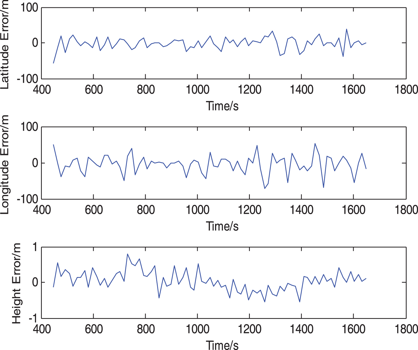
Figure 4. Results of non-adjustable-period method.

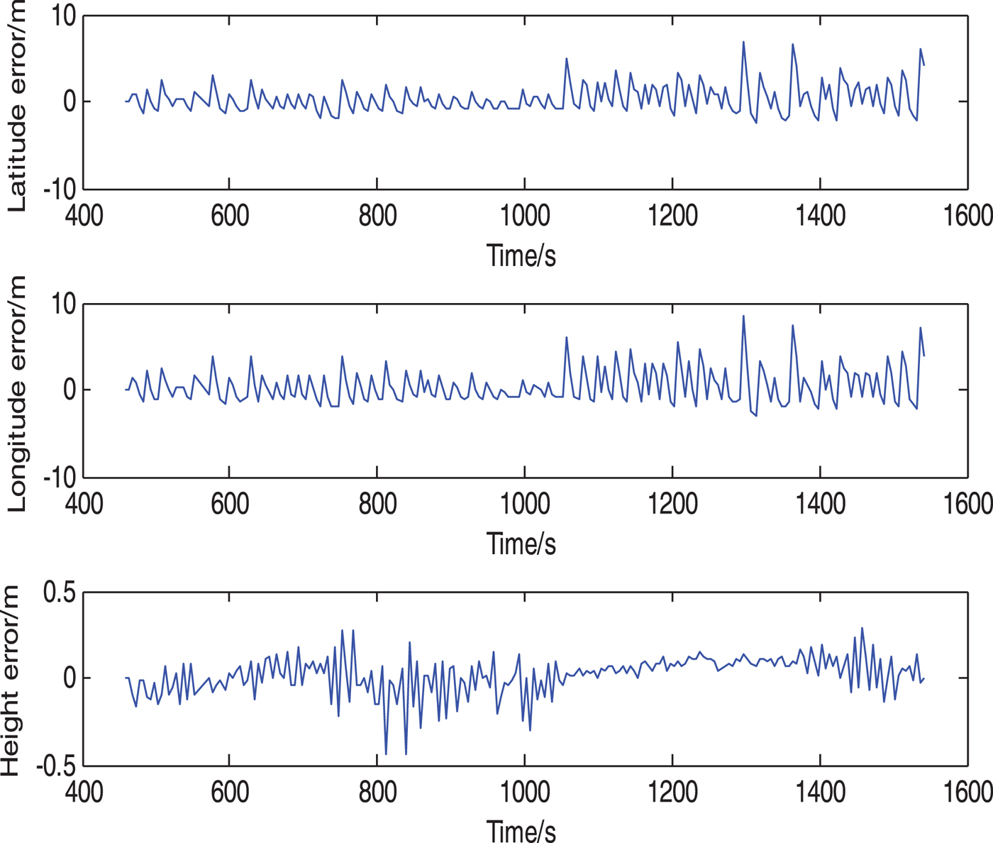
Figure 5. Results of the method in this paper.
In Figure 4, through the non-adjustable-period filtering method, the mean square error of latitude, longitude and height error are 5·82 m, 2·72 m and 0·26 m respectively. In Figure 5, using the presented method, the mean square error of latitude, longitude and height error are 1·96 m, 1·61 m and 0·11 m, which are only 33·7%, 59·2% and 42·3% of the mean square error through the non-adjustable-period filtering method respectively. Obviously, when the output signal periods of different sensors are certain, the filtering effect of the method in this paper is better than the effect of the non-adjustable-period filtering method.
The error accumulation of the compass and DVL would result in error accumulation in DR navigation. The integrated filtering based on the non-adjustable-period filtering method cannot fuse the data until it has calculated the lowest common multiple of output signal periods of all sensors and taken this as the filtering period (15 s in the experiment data here). Because of a relatively long integration period, the DR navigation error accumulates quickly, leading to heavy data fluctuation after integration. In contrast, the presented method can fuse the data immediately when valid data is generated, with an integration period of 5 s. Clearly, the DR navigation error is smaller over 5 s compared with 15 s. Therefore, data fluctuation becomes mild and the navigation output is smoother. The conclusion that the navigation precision of the method in this work is better than the non-adjustable-period filtering method can be drawn.
3.2. Experiment when output signal periods are time-varying
When the environment is complex, the output signal periods of the navigation sensors are time-varying. In this situation, the DR and integrated filtering method based on non-adjustable-period filtering is no longer applicable for data fusion. However, the presented method can adjust the filtering period in real time according to the period characteristic of the output signals. Based on analysis of the valid output signals, this paper mainly studies data fusion of various sensors when the output signal periods are time-varying. Finally, sea trial data is used to verify the effectiveness of the presented method.
3.2.1. Analysis of output signal periods
Another set of deep sea data whose output signal periods change frequently and largely was used to test the presented method. The experiment data contains output from of the compass, DVL, depth gauge and USBL. The whole experiment lasted for 1 hour and 20 minutes. The output periods of different sensors are shown in Figure 6.
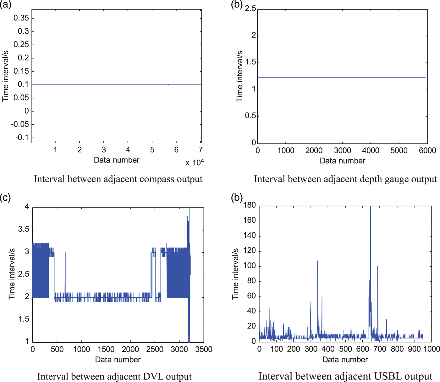
Figure 6. The interval of adjacent sensor valid output.
As seen in Figure 6, the compass period is 0·1 s and the depth gauge period is 1·23 s. The DVL period ranges from 1·9 s to 3·1 s with the middle section period of 2 s. Therefore, the reckoning period must be adjusted in real time during dead reckoning. The USBL period changes greatly from 4 s to 180 s. In Figure 6(d), the USBL period is 4 s in the forepart. Because of return signal delay or loss of valid data, the valid period is approximately in multiples of 4 s. In terms of acoustic transmission distance increase, the transmission period changes to 5 s, and then the valid USBL period is in multiples of approximately 5 s. Evidently, in practical application, the output signal periods of acoustic sensors are full of uncertainty. Thus, the method must determine the filtering period according to the time when the specific signals arrive.
As seen from analysis above, the DVL and USBL periods change frequently and greatly. The DR navigation period and Kalman filter period must be adjusted according to the arrival time of DVL and USBL signals.
3.2.2. Experiment when sensor output period is time-varying
The output signals of different sensors contain the corresponding time label. As shown in Figure 3, this work fuses the data of multi-sensor output signals based on signal trigger and time-space alignment to attain a high precision. This method considers the valid signals of the DVL as the trigger signals of the DR navigation program. It also considers the valid signals of acoustic positioning sensors as the trigger signals of an integrated navigation program. The corresponding time relative to the time label serves as the alignment reference. Because the output signal periods of the acoustic sensors are time-varying and the lowest common multiple of signal periods is uncertain, the non-adjustable-period filtering method cannot work on fusing the data here. Instead, it is filtered with the proposed method, results of which are shown in Figure 7.

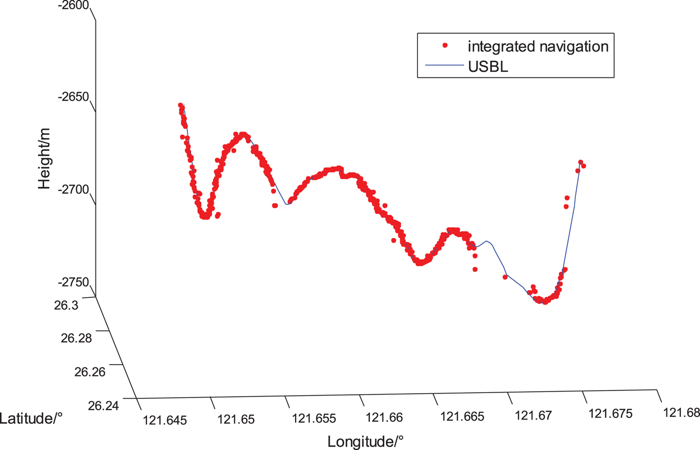
Figure 7. 3D position comparison of USBL and integrated navigation.
In Figure 7, the USBL data is the valid data extracted from all USBL data. The invalid USBL data exists because of external disturbances, making the period of valid data long and frequently changing. Navigation results indicate that the method proposed in this paper can calculate the three-dimensional position of the vehicle and reveal the actual trajectory.
4. CONCLUSION
By analysing the output characteristics of the compass, DVL, depth gauge and USBL, a multi-sensor integrated navigation and position method based on multi-stage signal trigger for an underwater vehicles is proposed in this paper, to deal with the problem that the output signals of the DVL and acoustic positioning sensor have different data intervals and period variations. Sea trial data based on Compass/DVL/USBL/Depth Gauge is processed by this method to verify its superiority when output signal periods are fixed and its validity when output signal periods are time-varying.
The velocity signal of the DVL is not the instantaneous value of the receiving time, but the average value of the whole signal period. Therefore, to improve the precision of the DR system, future work will be mainly focused on dynamically modifying the velocity signal of the DVL according to the speed of the vehicle.
ACKNOWLEDGEMENT
This work is supported by National Natural Science Foundation (NNSF) of China under Grant (61473019 and 61374210).