INTRODUCTION
The Patagonian Fjord Ecosystem (PFE) in southern Chile extends from Puerto Montt (41°20′S) to Cape Horn (55°58′S). This ecosystem is ~1600 km long and covers a total area of 240,000 km2 (Palma & Silva, Reference Palma and Silva2004).
Throughout the large Patagonian region, plankton communities are affected by high spatial heterogeneity due to strong seasonal, latitudinal and vertical variations in oceanographic conditions (Sievers et al., Reference Sievers, Calvete and Silva2002; Silva & Calvete, Reference Silva and Calvete2002; Palma & Silva, Reference Palma and Silva2004). These variations affect the composition, abundance and distribution of planktonic cnidarians (Palma et al., Reference Palma, Apablaza and Soto2007a, Reference Palma, Apablaza and Silvab, Reference Palma, Retamal, Silva and Silva2014a, Reference Palma, Córdova, Silva and Silvab; Villenas et al., Reference Villenas, Soto and Palma2009). Conspicuous zooplankton species previously reported (e.g. Muggiaea atlantica, Lensia conoidea, Clytia simplex, Euphausia vallentini, Sagitta tasmanica) have successfully adapted to an estuarine habitat, that is characterized by low levels of diversity, specific richness and abundance in comparison to the highly productive waters of the Humboldt Current System (Palma, Reference Palma1994; Palma & Rosales, Reference Palma and Rosales1995; Palma & Apablaza, Reference Palma and Apablaza2004; Pavez et al., Reference Pavez, Landaeta, Castro and Schneider2010).
The area between the Gulf of Penas and the Strait of Magellan experiences permanent inflow of Sub-Antarctic waters from the Pacific Ocean to the interior of the Patagonian Fjord Ecosystem, penetrating mainly through the Trinidad and Concepcion Channels and the Nelson and Magellan Straits. This more saline seawater mixes with the colder fresh water from rivers, coastal runoff, rainfall and glacial snowmelt (from the mountains and snowstorms), leading to a two-layer structure in the water system (Sievers & Silva, Reference Sievers, Silva, Silva and Palma2008). This leads to higher values of vertical stratification, associated with a strong pycnocline in the interior of the fjords and channels and lower stratification values in coastal waters close to the ocean (Bustos et al., Reference Bustos, Landaeta and Balbontín2011).
However, the sector between the Trinidad Channel (50°10′S) and the mouth of the Strait of Magellan (52°45′S) has remained poorly studied. The first studies of zooplankton were obtained during the RV ‘Hero’ Expedition (1972–1973), reporting some species of copepods, euphausiids and chaetognaths (Arcos, Reference Arcos1974, Reference Arcos1976; Ahumada, Reference Ahumada1976; Antezana, Reference Antezana and Orrego1976). Later, during the CIMAR-2 Fjord Cruise (spring of 1996), the analysis was focused particularly on siphonophores, chaetognaths, cladocera and euphausiids (Palma et al., Reference Palma, Ulloa and Linacre1999; Rosenberg & Palma, Reference Rosenberg and Palma2003). A total of nine siphonophore species were identified, of which Muggiaea atlantica and Lensia conoidea were dominant (Palma et al., Reference Palma, Ulloa and Linacre1999). Both species are found widely distributed through the Patagonian Fjord Ecosystem, with the highest numbers of M. atlantica showing a positive correlation with temperatures associated with the adjacent Pacific Ocean waters and a preferentially surface bathymetric distribution (0–50 m). The highest number of L. conoidea show a positive correlation with salinity and density, and a deeper bathymetric distribution (>50 m) (Palma et al., Reference Palma, Ulloa and Linacre1999, Reference Palma, Silva, Retamal and Castro2011).
The objective of the present study is to characterize the composition, abundance, horizontal and vertical distributions of the siphonophore community and to test the hypothesis that the strong environmental gradient found in this ecosystem shapes the abundances and community composition of siphonophores in this poorly known area.
MATERIALS AND METHODS
During the marine research cruises in remote areas (CIMAR-15), carried out aboard the RV ‘Vidal Gormaz’, 28 oceanographic stations were set up in the fjords and channels between the Trinidad Channel (50°06′S) and the mouth of the Strait of Magellan (52°45′S) between 11 October and 10 November 2009 (Figure 1). Of those stations, 13 were selected to build a north-south oceanographic cross-section close to the western edge of the Southern Ice Fields (Figure 1, blue line).

Fig. 1. Geographic position of sampling stations between the Trinidad Channel and Magellan Strait (CIMAR 15 Fiordos cruise). The blue line indicates the longitudinal north-south transect.
At each station temperature and salinity were recorded with a CTD Seabird SB-19, from the surface up to a depth of 500 m or to 10 m from the ocean floor (depending on the depth of the station). Discrete water samples were also taken using a rosette fitted with 24 Niskin bottles to determine dissolved oxygen concentration at standard depths (0, 2, 5, 10, 25, 50, 75 and 100 m) by the Winkler method as modified by Carpenter (Reference Carpenter1965).
Zooplankton samples were collected by oblique tows at three depth strata: surface (0–25 m), middle (25–50 m) and deep (50–100 or 200 m, depending on the bottom depth); using a Tucker trawl net (1 m2 mouth opening and 350 µm mesh aperture) and a digital flowmeter to estimate the volume filtered by each net. Zooplankton samples were fixed immediately after collection and preserved in 5% formalin buffered with sodium borate.
The siphonophores were sorted and the nectophores (asexual polygastric stage) and eudoxids (sexual eudoxid stage) were identified and counted. The taxonomic identification followed the work of Totton (Reference Totton1965) and Pugh (Reference Pugh and Boltovskoy1999). The abundances of Calycophorae were estimated considering the highest number of anterior and posterior nectophores (asexual polygastric stage), and bracts and entire eudoxids (sexual eudoxid stage). Pyrostephos vanhoeffeni was the only species of the Physonectae collected, and its abundance was estimated by considering one individual to have 20 pairs of nectophores per colony (Totton, Reference Totton1965). Data of polygastric and eudoxid stages were considered separately for Muggiaea atlantica and Lensia conoidea. Zooplankton abundance was standardized to individuals per 1000 m3.
Two indices commonly used to describe the siphonophore community (Palma et al., Reference Palma, Apablaza and Soto2007a, Reference Palma, Apablaza and Silvab, Reference Palma, Silva, Retamal and Castro2011, Reference Palma, Retamal, Silva and Silva2014a, Reference Palma, Córdova, Silva and Silvab) are dominance (DO), calculated as the percentage of each species over the total individuals collected and frequency of occurrence (FO), which is the percentage of the presence of each species over the total number of stations sampled. Only the dominant species (DO > 5% of the total collected specimens) were considered to describe the horizontal and vertical distribution patterns.
Temperature, salinity and dissolved oxygen concentration were used to determine the oceanographic characteristics of the study zone. However, as these variables are measured at different depths than zooplankton samples, the weighted means of the environmental variables were calculated for the zooplankton samples range, following:
 $$X_{ij}\displaystyle{{\sum {Z_{\,jk} \ast C_{ijk}}} \over {\sum {Z_{\,jk}}}} $$
where X ij is the weighted mean of the i-th parameter at the j-th station, Z jk is the k-th depth at the j-th station, C ijk is the mean of the i-th parameters of the delta of the k-th depths at the j-th station.
The siphonophore community structure was characterized using non-metric multi-dimensional scaling (nMDS) (Clarke & Warwick, Reference Clarke and Warwick1994). The abundance data were transformed by the fourth root to reduce the contribution of the most abundant species and increase the contribution of rarer species. In order to test for significant differences among discrete groups coming from the nMDS analysis, the ANOSIM procedure was used (Clarke & Warwick, Reference Clarke and Warwick1994). The association of the community structure with the environmental variables was achieved using canonical correspondence analysis (CCA) (Ter Braak, Reference Ter Braak1986). This analysis involved searching for correlations between species abundance and the environmental data considering species unimodal responses. In order to find the most parsimonious model (highest inertia explained by only significant explanatory variables) a forward stepwise model selection was performed using permutation tests. For the canonical correspondence analysis and for the permutations test the functions cca and ordistep, respectively, from the ‘vegan’ package were used (Oksanen et al., Reference Oksanen, Blanchet, Kindt, Legendre, Minchin, O'Hara, Simpson, Peter Solymos, Henry, Stevens and Wagner2015).
The association between environmental variables and each dominant species (DO > 5%) was evaluated through regression analysis. Due to the nature of species data (i.e. count numbers) and to avoid data transformation, generalized linear models (GLMs) with a binomial negative error family distribution and a log ‘link’ function were fitted using the glm.nb function from the ‘MASS’ package (Venables & Ripley, Reference Venables and Ripley2002). The volume sampled (log-transformed) was used as an offset inside the GLMs because of its high variability between stations (data not shown; Guerrero et al., Reference Guerrero, Gili, Rodriguez, Araujo, Canepa, Calbet, Genzano, Mianzan and González2013). The optimal model was achieved using a backward selection procedure until all explanatory variables were significant (Zuur et al., Reference Zuur, Ieno, Walker, Saveliev and Smith2009). To avoid collinearity (i.e. significant correlation among environmental variables), a pairwise comparison between each explanatory variable was carried out using the Spearman rank correlation coefficient (rho). When the coefficient value was higher than 0.6, the less (biologically) important variable was removed from the analysis (Zuur et al., Reference Zuur, Ieno and Elphick2010). All the statistical tests used were conducted in the free programming language R, version 3.2.1 (R Core Team, 2015).
The vertical distribution of the dominant species was analysed along a longitudinal north-south transect composed of 13 stations located between the Peel Fjord (Station 73) and the south end of the Smyth Channel (Station 61) (Figure 1). The vertical transect for temperature, salinity and dissolved oxygen was built using a Kriging function with linear interpolation in the software package Surfer 8.0.
Finally, the inter-annual abundance of the siphonophores (polygastric stage) collected during the cruises CIMAR 2 Fiordos (C2F, 15 October to 4 November 1996; Palma et al., Reference Palma, Ulloa and Linacre1999) and CIMAR 15 Fiordos (C15F, 11 October to 10 November 2009) was compared using only those stations with the same geographic location. To quantify significant differences in average siphonophorae abundance between the two datasets, GLMs similar to those used for the environmental association were fitted (i.e. GLM with a negative binomial error family distribution and a log link function). It is important to highlight that both cruises were done during the same months of the year (October–November), and in the cruise C2F we used Bongo nets and in the cruise C15F we used Tacker Trawls nets, but in both cruises we compared the standardized values of abundance of polygastric phase (i.e. nectophores).
RESULTS
Hydrography
The longitudinal transect from Peel Fjord to Smith Channel presented an inverted thermal vertical distribution with the lower temperatures (5–7°C) in the surface layer (0–50 m) (Figure 2A). A weak inverted thermocline (≈−0.08°C m−1) centred around 35 m was present around Peel Fjord (Stations 72–73; Figure 2A). The salinity showed a stratified low saline (26–32) surface layer, with high dissolved oxygen content (6–8 ml l–1) (Figure 2B, C). The halocline (≈0.15 m−1) was centred at about 35 m depth, in the Collingwood–Smyth Fjords junction (Stations 63–66; Figure 2B). The deep layer (50 m to bottom) was less stratified, warmer (8–9°C), more saline (32–33) and less oxygenated (3–6 ml l–1), than the surface layer (Figure 2A–C).

Fig. 2. Vertical distribution of (A) temperature, (B) salinity and (C) dissolved oxygen in the longitudinal north-south transect between Trinidad Channel and Magellan Strait in spring 2009.
Siphonophore species composition
A total of 10 species of siphonophores (polygastric and eudoxid stages), nine calycophorans and one physonect were identified. Agalma elegans was recorded for the first time in the Patagonian Fjord Ecosystem (PFE), and Rosacea plicata and Sphaeronectes fragilis were recorded for the first time in this geographic area. Disregarding the eudoxid stages, four dominant species (DO > 5%) were found with very similar abundance percentages: Lensia conoidea (26.3%), Dimophyes arctica (24.6%), Lensia meteori (22.2%) and Muggiaea atlantica (20.7%). The other species accounted for only 6.2% of the total. For the eudoxid stage, the highest densities were found for L. conoidea (57.2%) and D. arctica (40.1%) (Table 1).
Table 1. Summary of basic statistics for polygastric (po) and eudoxids (eu) stages of siphonophores. Total number of individuals, range of non-zero abundances, average per station, dominance and occurrence were calculated for polygastric and eudoxid stages separately. Abundances are expressed as ind. 1000 m −3.
Asterisk indicates the dominant species. Ne, nectophores.
Horizontal distribution patterns of siphonophores
The abundances of siphonophores ranged between 11 ind. 1000 m−3 in the Concepcion Channel (Station 41) and 3080 ind. 1000 m−3 in the Collingwood Strait (Station 65), with an average per station of 65.7 ind. 1000 m−3. The highest densities were found in the Collingwood Strait (Stations 65 and 66) and the lowest densities were found in the Concepcion Channel (Stations 41 and 42).
Lensia conoidea was the most abundant species and showed the greatest geographic coverage (FO = 79%). Its non-zero range of abundance (NZRA) fluctuated between 5 and 865 ind. 1000 m−3 in Concepcion (Station 41) and the Sarmiento Channel (Station 68), respectively (Table 1). The highest densities were found in the Smyth and Sarmiento Channels and the lowest densities (even reached zero) in oceanic waters and areas close to the head of the fjords (e.g. Europa, Peel and Las Montañas Fjords) (Figure 3A). Dimophyes arctica (DO = 24.6%) was found only in interior waters and its NZRA varied from 18 to 806 ind. 1000 m−3 around Europa (Station 36) and the Peel Estuary (Station 72), respectively (Table 1). The highest densities were found in the Peel Fjord, and the Smyth and Kirke Channels (Figure 3B). Similar to D. arctica, L. meteori (DO = 22.2%) was present only in interior waters south of 51°S, with low abundances and a minimum of 4 and a maximum of 2085 ind. 1000 m−3 in the Smyth Channel (Station 48) and Collingwood Strait (Station 65), respectively. Besides this, L. meteori was mainly present in Station 65, where 50% of the total nectophores were collected (Figure 3C). Finally, despite having the lowest abundance among the dominant species, M. atlantica (DO = 20.7%) had the highest geographic coverage with a high frequency of occurrence (FO = 93%). Its NZRA fluctuated between 6 and 756 ind. 1000 m−3 in the Concepcion (Station 43) and Smyth Channels (Station 50) (Figure 3D), respectively. Among the occasional species (DO < 5%), P. vanhoeffeni showed high geographic coverage through the study zone (FO = 61%).

Fig. 3. Horizontal distribution of polygastric stages during spring 2009. (A) Lensia conoidea; (B) Dimophyes arctica; (C) Lensia meteori and (D) Muggiaea atlantica.
The eudoxids of L. conoidea (DO = 57.2%) and D. arctica (DO = 40.1%) were always more numerous than the polygastric stages, with average densities seven and four times higher than their respective polygastric stages, respectively. These eudoxids followed the same abundance patterns as the polygastric stage, though the highest abundances were found in the fjords (Figure 4A, B). In the case of L. conoidea, the highest accumulations of eudoxids (>4900 ind. 1000 m−3) were found in the Europa Fjord (Stations 36 and 38, Figure 4A), while for D. arctica, the highest accumulations (>1100 ind. 1000 m−3) were found in the Peel Fjord (Stations 70–74, Figure 4B).

Fig. 4. Horizontal distribution of eudoxid stages during spring 2009; (A) Lensia conoidea and (B) Dimophyes arctica.
Community structure of siphonophores
The nMDS community association analysis (0.13 stress) grouped the oceanographic stations in three areas with contrasting community structures. The first group (Group 1) contained 22 stations associated to estuarine waters located in the fjords (Europa, Peel and Las Montañas) and along the channels (Sarmiento and the Smyth Channel (except Station 61) and was characterized by low values of temperature, salinity and high vertical stratification. Group 2 represented stations associated to the high exchange between estuarine and oceanic waters. It was comprised of three stations, two located in the northern part of the Concepcion Channel (Stations 41 and 42) and one in the southern end of the Smyth Channel (Station 61). Finally Group 3 had only two stations and clearly associated to oceanic waters (Stations 43 and 44) (Figure 5). The stations of Groups 2 and 3 were characterized by higher values of temperature and salinity, and lower vertical stratification, because they represented well mixed waters, but at the same time with low siphonophore abundance. The pairwise tests of ANOSIM analysis showed high dissimilarity due to the differences in oceanographic conditions in the three groups (Group 1, 2: R = 0.856; Group 1, 3: R = 0.936, and Group 2, 3: R = 1; P < 0.001; Table 2).

Fig. 5. Non-metric multidimensional scaling (nMDS) based on Bray–Curtis similarity index of the total siphonophore species collected. Group 1: species of estuarine waters; Group 2: species with oceanic influence; and Group 3: species of oceanic waters (spring 2009). Stress: 0.13.
Table 2. Results of the ANOSIM using the pairwise tests.
Environmental associations
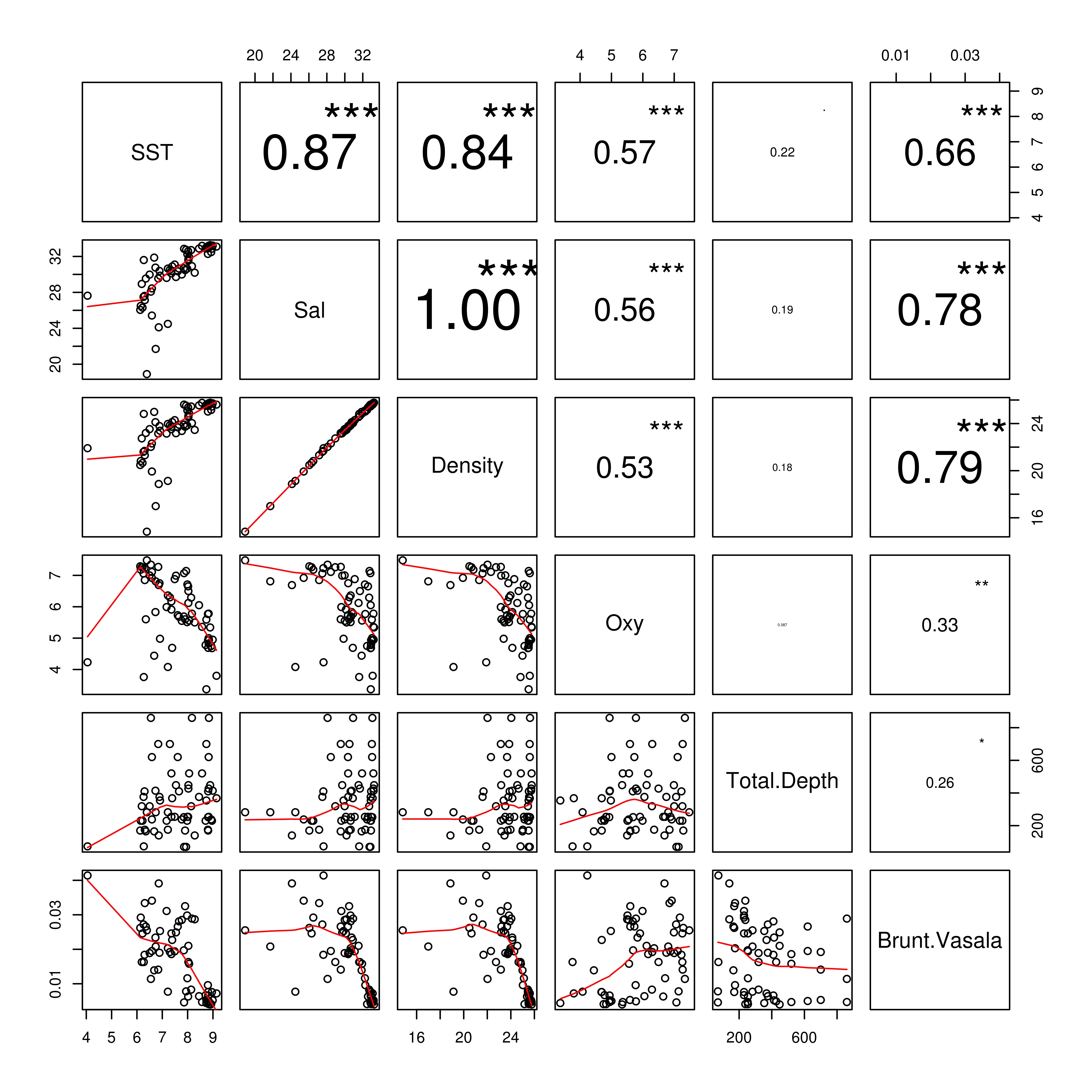
The environmental variables for which multiple comparisons showed a Spearman rank correlation coefficient (rho) lower than 0.6 (e.g. Temperature, Salinity, Dissolved Oxygen) were kept to run the statistical models of species–environmental association (online Figure S1).
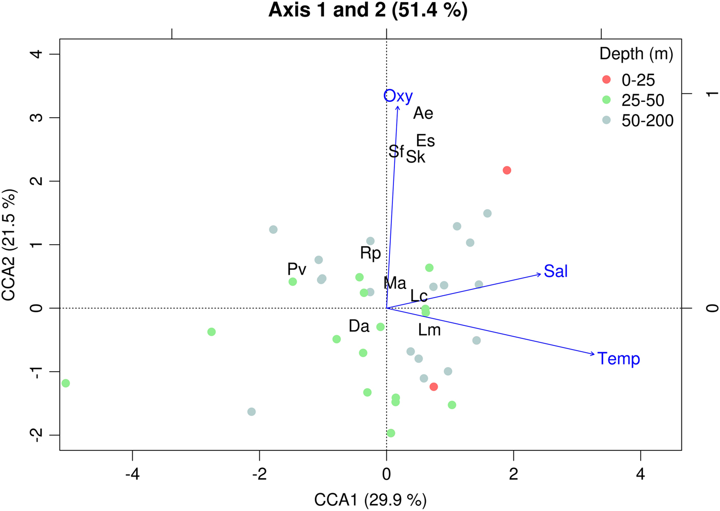
Temperature and dissolved oxygen played a significant role in the deviance (univariate) and inertia (multivariate) data (Tables 3 & 4). The dominant species (DO > 5%) showed a positive and significant response to temperature with a non-linear response (except for the case of M. atlantica) (i.e. significant quadratic term in GLMs; Table 2; Figure 6). On the other hand, the siphonophores species (except L. meteori) related negatively to dissolved oxygen (Table 2, Figure 6). From the multivariate perspective, the most parsimonious model explained a total inertia of 51.4%, where the first axis (CCA x-axis) explained more inertia than the second (CCA y-axis) axis, 29.9 and 21.5%, respectively. From the triplot analysis (scaling 2), the negative association between dissolved oxygen and the dominant species was also evident (Figure 7). A remarkably positive association with dissolved oxygen was evident for the group of non-dominant species (S. fragilis, S. koellikeri, E. spiralis and A. elegans; Figure 7).
Fig. 6. Relationships of dominant siphonophore species with significant environmental variables from the generalized linear models (GLM).

Fig. 7. Canonical Correspondence Analysis triplot (scaling 2) based on data from spring 2009 showing the distribution of sampling stations (points, N = 40) by depth strata, siphonophore species (black labels, N = 10) and environmental variables (blue arrows). The total explained inertia (51.4%), and partial explained inertia per axis is also shown. Lc: Lensia conoidea; Da: Dimophyes arctica; Lm: Lensia meteori; Ma: Muggiaea atlantica; Pv: Pyrostephos vanhoeffeni; Sk: Sphaeronectes koellikeri; Sf: Sphaeronectes fragilis; Rp: Rosacea plicata; Es: Eudoxoides spiralis; Ae: Agalma elegans. Temp: temperature; Sal: salinity; Oxy: dissolved oxygen.
Table 3. Summary statistics of the generalized linear models (GLM) for each dominant species of Siphonophorae.

Values of the statistical test (Z-test from a binomial negative error family distribution and a log ‘link’), explained deviance and significance are shown. T, temperature; DIO, dissolved oxygen.
*P < 0.05; **P < 0.01; ns, non-significant.
Vertical distribution in the north–south transect
The vertical distribution of the dominant species (only polygastric stage) showed different patterns along the north-south transect (Figure 1, blue line). Muggiaea atlantica had a frequency of occurrence (FO) of 100% along the transect and showed deeper populations along the north-south gradient (Figure 8D). In the Peel Fjord it was collected mainly in the surface layer (0–25 m), in the Sarmiento Channel it was found mainly in the middle layer (25–50 m), and along the Smyth Channel it was collected mainly in the deep layer (>50 m), particularly at the most southern stations close to the Pacific. In the Peel Fjord, L. conoidea (FO = 92.3%) showed a uniform vertical distribution pattern, while in the Sarmiento and Smyth Channels it was collected mainly in the deep layer (50–200 m) (Figure 8A). Dimophyes arctica (FO = 84.6%) behaved similarly to M. atlantica, as it also moved deeper along the north-south gradient (Figure 8B). In the Peel Fjord it was found mostly in the surface layer, in the Sarmiento Channel in the middle layer and the deep layer, also moving deeper towards the stations with more oceanic characteristics (Figure 8B). In the Peel Fjord, L. meteori (FO = 84.6%) was found mainly in the surface and middle layers (0–50 m), while in the Sarmiento and Smyth Channels it was mainly collected in the deep layer (Figure 8C).

Fig. 8. Vertical distribution of dominant species: (A) Lensia conoidea; (B) Dimophyes arctica; (C) Lensia meteori; and (D) Muggiaea atlantica in a longitudinal north-south transect between Trinidad Channel and Magellan Strait in spring 2009. Grey boxes: diurnal tows, black boxes: nocturnal tows.
Inter-annual comparison between the abundance of siphonophores in springs of 1996 and 2009
Comparisons of weighted temperature, salinity and dissolved oxygen data between C2F and C15F (Figure 9) showed that salinity and dissolved oxygen do not show inter-annual differences. Nevertheless, surface temperature does not completely follow this pattern, since for C15F the surface layer (0–25 m) was significantly colder than for C2F (≈1°C; Figure 9).
Fig. 9. Comparison of temperature, salinity and dissolved oxygen among different depths for both spring seasons (Cruises CIMAR 2–15 Fiordos).
A total of seven siphonophore species were identified in the spring of 1996 and 10 in the spring of 2009. The dominant species for both periods were Lensia conoidea (DO = 52.2 and 26.8%), L. meteori (DO = 7.4 and 24.2%), Muggiaea atlantica (DO = 35.4 and 21.1%) and Dimophyes arctica (DO = 22.5 and 3.8% (not dominant)) in the springs of 1996 and 2009, respectively (Table 5).
In spring 1996, the abundance values fluctuated between 5 and 2413 ind. 1000 m−3, with the highest densities located in the northern part of the Sarmiento Channel. In the spring of 2009, the abundance varied between 10 and 4386 ind. 1000 m−3, with the highest densities recorded in the Collingwood Strait, south of the Sarmiento Channel (Table 4). The higher average abundance in 2009 (626.8 ind. 1000 m−3) compared with 1996 (177.7 ind. 1000 m−3) was strongly significant (Z = 3.93, P < 0.01, Table 6).
Table 4. Results of the permutation test for the canonical correspondence analysis (51.4% of explained inertia) for the siphonophorae community.
Values of the statistical test (F-value) and significance (P) for the global test and for each explanatory variable are shown.
Table 5. Summary of statistics for the nectophores collected between springs 1996 and 2009. Total number of individuals, range of non-zero abundances, average per station, dominance and occurrence are shown. Abundances are expressed as ind. 1000 m−3.
Asterisks indicate the dominant species of siphonophores in both spring seasons.
Table 6. Summary statistics of the generalized linear models (GLM) for the comparisons of average abundance between years 1996 and 2009.

– Species not registered in spring 1996.
Values of the statistical test (Z-test from a negative binomial distribution with a link = ‘log’) and significance are shown.
a Dominant species, bold font: significant differences between years.
The mean abundance of L. conoidea in 2009 was 1.8 times higher than in 1996 (169 vs 93 ind. 1000 m−3), though this difference was not significant (Z = 1.12; P = 0.26). This species was absent from the collections at stations with greater influence from oceanic waters and in the Kirke Channel. In both periods, the highest densities were recorded in the Europa and Peel Fjords, and in the Sarmiento and Smyth Channels. Lensia meteori was significantly more abundant in 2009 than in 1996 (11.6 times; 24.2 vs 7.4 ind. 1000 m−3) (Z = 3.46; P < 0.01). Its geographic distribution in 1996 showed low coverage, while in 2009 its abundance increased south of 51°S, particularly in the Collingwood Strait. Dimophyes arctica was 21 times more abundant in 2009 than in 1996 (22.5 vs 3.8 ind. 1000 m−3) (Z = 5.33; P < 0.01). Its geographic distribution was very similar to that of L. meteori, though its high abundance was found in the Peel Fjord and Sarmiento and Smyth channels. It was particularly absent from stations with greater influence from oceanic waters. Finally, M. atlantica was the second most dominant species in 1996, while in 2009 it showed the lowest abundance of the dominant species. Although its geographic distribution was similar for both periods, its geographic coverage was much higher in 2009 (FO = 67 vs 93%). Its mean abundance was 2.1 times higher in 2009 (Z = 1.46; P < 0.01), particularly in association with the Sarmiento and Smyth channels (Figure 3). Other (non-dominant) species that showed significant increases from 1996 to 2009 were Pyrostephos vanhoeffeni (Z = 5.39; P < 0.01) and Eudoxoides spiralis (Z = 6.32; P < 0.01) (Table 6).
DISCUSSION
Agalma elegans was recorded for the first time in the Patagonian Fjord Ecosystem (PFE). Rosacea plicata and Sphaeronectes fragilis were recorded for the first time in this geographic area (50°10′–52°45′S), but these species have been recorded previously in other areas of the PFE (Palma & Silva, Reference Palma and Silva2004; Palma et al., Reference Palma, Apablaza and Soto2007a, Reference Palma, Silva, Retamal and Castro2011, Reference Palma, Retamal, Silva and Silva2014a; Villenas et al., Reference Villenas, Soto and Palma2009). The highest siphonophore densities were found in estuarine waters, where all the dominant species were recorded (i.e. Lensia conoidea, Dimophyes arctica, L. meteori and Muggiaea atlantica). The lowest densities were found in the exterior zone influenced by the adjacent Pacific Ocean and characterized by the presence of occasional species (i.e. Sphaeronectes fragilis, Agalma elegans, Sphaeronectes koellikeri and Eudoxoides spiralis). The vertical distribution patterns of the dominant species showed that M. atlantica was distributed shallower (0–50 m) than L. conoidea, D. arctica and L. meteori, which were collected mostly in the deeper layer (below 50 m).
Siphonophore community composition and horizontal distribution
The community structure of the siphonophores between the Trinidad Channel and the Strait of Magellan had only been studied in the spring (October–November) of 1996 during the CIMAR-2 Fiordos cruise (Palma et al., Reference Palma, Ulloa and Linacre1999). In general, this area is characterized by low values of species richness with 7 and 10 species for the springs of 1996 (Palma et al., Reference Palma, Ulloa and Linacre1999) and 2009 (this study). These low species richness values confirm the results obtained for different zooplankton groups in the Patagonian Fjord Ecosystem (Puerto Montt to Cape Horn) in comparison to the waters of the Humboldt Current System (Palma, Reference Palma, Silva and Palma2008). Most of the species identified are frequent in the PFE (Palma & Silva, Reference Palma and Silva2004; Palma et al., Reference Palma, Silva, Retamal and Castro2011, Reference Palma, Retamal, Silva and Silva2014a) and are common in Antarctic waters (i.e. Dimophyes arctica, Pyrostephos vanhoeffeni) and in Sub-Antarctic waters (Agalma elegans, Eudoxoides spiralis, Lensia conoidea, L. meteori, Muggiaea atlantica, Rosacea plicata, Sphaeronectes fragilis and S. koellikeri), respectively.
The three occasional species (A. elegans, R. plicata and S. fragilis) constitute new records for the study zone. Some nectophores of A. elegans were collected in some stations, becoming the first record for the PFE. However R. plicata and S. fragilis has been collected in other areas of the PFE, as a Chiloé Interior Sea and Magellanic Region (Pagès & Orejas, Reference Pagès and Orejas1999; Palma & Silva, Reference Palma and Silva2004; Palma et al., Reference Palma, Apablaza and Soto2007a). Some colonies of the Antarctic physonect P. vanhoeffeni, though not abundant, are widely distributed in the study area, showing increased geographic coverage compared with the spring of 1996, when it was collected exclusively in low temperature and low salinity estuarine waters (Palma et al., Reference Palma, Ulloa and Linacre1999). An incidental occurrence of this species was recorded off Valparaíso (33°S; Palma, Reference Palma1986).
Lensia conoidea was the dominant species, showing wide geographic coverage over the study area, with maximum abundance values in estuarine waters (Sarmiento and Smyth Channels) and absence from most of the oceanic stations. The eudoxid stages were collected at the same stations as the polygastric stages, but the highest aggregations of individuals were recorded in the Europa Fjord. This species is very common and frequent in the PFE (Palma et al., Reference Palma, Ulloa and Linacre1999, Reference Palma, Apablaza and Soto2007a, Reference Palma, Silva, Retamal and Castro2011, Reference Palma, Retamal, Silva and Silva2014a; Palma & Silva, Reference Palma and Silva2004). However, in the HCS it has been recorded only once in the bay of Valparaiso (Palma, Reference Palma1973). This species is common and abundant in the great oceans, especially in the California and Benguela currents, and in the Mediterranean Sea, spanning broad depth distributions from the surface down to the pelagic zone (Alvariño, Reference Alvariño1971; Pugh, Reference Pugh1984, Reference Pugh and Boltovskoy1999; Kirkpatrick & Pugh, Reference Kirkpatrick and Pugh1984). It has been recorded also in other fjord ecosystems like Korsfjord Fjord in Norway (Hosia & Båmsted, Reference Hosia and Båmstedt2008).
Dimophyes arctica was the second most dominant species and it was collected mainly in estuarine waters (Peel Fjord and Sarmiento and Smyth channels), i.e. water with low temperature (<6°C) and salinity (<30). The eudoxid stages were collected at the same stations as the polygastric stages, but the highest aggregations of eudoxids were recorded in the Peel Fjord. Its abundance is very low with an irregular distribution in the PFE and its abundance increasing from Puerto Montt to Cape Horn (Palma & Silva, Reference Palma and Silva2004; Palma, Reference Palma, Silva and Palma2008). This species is common in epipelagic Antarctic and Sub-Antarctic waters transported by the West Wind Drift Current that enters the PFE (Palma & Silva, Reference Palma and Silva2004). Dimophyes arctica is a cosmopolitan species, inhabiting the great oceans and the Antarctic, Arctic, the Mediterranean Sea and boreal fjords (Alvariño, Reference Alvariño1971; Hosia et al., Reference Hosia, Stemmann and Youngbluth2008). In boreal and austral latitudes it is more abundant in epipelagic waters than in tropical and temperate waters, where it is more common in meso- and bathypelagic waters (Pugh, Reference Pugh1984).
Lensia meteori was found at low density at most stations located in estuarine waters, with a maximum value in the Sarmiento Channel (Station 65) and absence from all oceanic stations. In Chilean waters it has been collected exclusively in the PFE, between Penas Gulf (50°S) and the Strait of Magellan (53°S) (Palma et al., Reference Palma, Ulloa and Linacre1999, and this study). This species inhabits temperate regions in the three great oceans and in the Mediterranean Sea and has a broad vertical distribution extending down to depths of 800 m (Alvariño, Reference Alvariño1971; Bouillon et al., Reference Bouillon, Medel, Pagès, Gili, Boero and Gravili2004).
Despite having the lowest abundance among the dominant species, M. atlantica showed high frequency of occurrence (FO = 90%) throughout the study zone. However, there is a notable lack of eudoxids collected in comparison to the number of nectophores (eudoxids:nectophores = 1:5), because in the Patagonian Fjord Ecosystem (PFE) we registered high densities of eudoxids in the same period, in spring 2008 between the Gulf of Penas (47°S) to Trinidad Channel (50°10′S) with superficial temperatures <9°C (Palma et al., Reference Palma, Retamal, Silva and Silva2014a). Beside this, in the south extreme of PFE, in the Magellan Region (52–56°S), the highest densities of eudoxids of M. atlantica occur in the Almirantazgo Sound, where the superficial temperature is <7°C (Palma & Aravena, Reference Palma and Aravena2001; Valdenegro & Silva, Reference Valdenegro and Silva2003). In this sense, recently Blackett et al. (Reference Blackett, Lucas, Harmer and Licandro2015) found that the populations of M. atlantica appear to have a temperature threshold of 10°C for the eudoxid production in the western English Channel. This ratio is generally the inverse in spring among dominant species, as observed with L. conoidea and D. arctica in the present study, and as shown by other results obtained in the PFE (Palma & Silva, Reference Palma and Silva2004; Palma et al., Reference Palma, Apablaza and Soto2007a, Reference Palma, Retamal, Silva and Silva2014a). Muggiaea atlantica is eurythermal and euryhaline, and is widespread in both the adjacent oceanic waters of the Pacific Ocean (SAAW) and in the FPE (MSAAW and EW) throughout the study area. This species is the most common and frequent siphonophore in the HCS (Palma, Reference Palma1973, Reference Palma1994; Palma & Rosales, Reference Palma and Rosales1995; Palma & Apablaza, Reference Palma and Apablaza2004; Pavez et al., Reference Pavez, Landaeta, Castro and Schneider2010) and in the PFE (Palma & Silva, Reference Palma and Silva2004; Palma et al., Reference Palma, Apablaza and Soto2007a, Reference Palma, Silva, Retamal and Castro2011, Reference Palma, Retamal, Silva and Silva2014a; Palma, Reference Palma, Silva and Palma2008; Villenas et al., Reference Villenas, Soto and Palma2009). Muggiaea atlantica is a neritic species inhabiting warm and temperate regions in the great oceans and in the Mediterranean Sea (Alvariño, Reference Alvariño1971; Bouillon et al., Reference Bouillon, Medel, Pagès, Gili, Boero and Gravili2004).
With regard to the reproductive process of L. conoidea and D. arctica, the highest eudoxid densities were recorded in the interior of the fjords. The highest aggregations of eudoxids of L. conoidea were recorded in the Europa Fjord, while for D. arctica this occurred in the Peel Fjord. This would mean better division of the area and its resources, leading to greater reproductive success. In the PFE, it has been seen that the fjords appear to be favourable to reproduction, displaying high concentrations of phytoplankton that would give higher food availability in such areas (Palma et al., Reference Palma, Retamal, Silva and Silva2014a, Reference Palma, Córdova, Silva and Silvab).
Environmental associations and vertical distribution
The nMDS and ANOSIM analysis, for the community structure, recognized three major groups of sampling stations (Figure 5). Group 1 was characterized by the abundance of those dominant species (D. arctica, L conoidea, L. meteori and M. atlantica). Of these species, D. arctica and L. conoidea presented the highest abundances in the estuarine waters. These species are widely distributed through the PFE, particularly M. atlantica and L. conoidea (Palma & Silva, Reference Palma and Silva2004; Palma et al., Reference Palma, Apablaza and Soto2007a, Reference Palma, Silva, Retamal and Castro2011, Reference Palma, Retamal, Silva and Silva2014a; Villenas et al., Reference Villenas, Soto and Palma2009). Group 2 was characterized by M. atlantica and L. conoidea but in low densities and Group 3 was characterized by the presence of occasional species (S. fragilis, A. elegans, S. koellikeri and E. spiralis) which are also occasional inhabitants of the PFE (Palma & Silva, Reference Palma and Silva2004; Palma et al., Reference Palma, Apablaza and Soto2007a, Reference Palma, Silva, Retamal and Castro2011, Reference Palma, Retamal, Silva and Silva2014a; Villenas et al., Reference Villenas, Soto and Palma2009). Of these occasional species, only S. koellikeri is abundant along the Chilean coast, where it is found in association with M. atlantica (Palma, Reference Palma1994; Palma & Rosales, Reference Palma and Rosales1995; Pavez et al., Reference Pavez, Landaeta, Castro and Schneider2010).
Both the univariate and multivariate analysis showed a positive association with temperature and a negative association with dissolved oxygen. The positive association with temperature has been previously demonstrated for M. atlantica (Palma et al., Reference Palma, Ulloa and Linacre1999; Palma & Silva, Reference Palma and Silva2004). The negative association with dissolved oxygen for L. conoidea (Palma & Silva, Reference Palma and Silva2004) was attributed to the presence of Equatorial Sub Superficial Waters (ESSW), demonstrating that even when those species are present in a wide range of environmental conditions, their maximum abundances are restricted to particular conditions.
Muggiaea atlantica presented broad vertical distribution throughout the study zone, though the highest concentrations of nectophores occurred in the surface and middle layers (Figure 8D). This layer (0–50 m) is associated with EW and has higher vertical stability in the water column, low temperature and salinity, and high values of dissolved oxygen. Its lower limit is determined by a strong halocline located at that depth which separates the EW from the deeper water (below 30 m), known as Modified Sub-Antarctic Water (MSAAW). The polygastric stages of L. conoidea, D. arctica and L. meteori were preferentially distributed in deeper waters (below 50 m). They were found in the surface layer in the Peel Fjord, but moved deeper from the Sarmiento Channel until south of the Smyth Channel, with the exception of Stations 61–63, where D. arctica and L. meteori were in fact absent (Figure 8A–C). These species were associated with the predominantly MSAAW in the deeper layer (depths of 50–200 m), characterized by quasi-homogeneous conditions for temperature, salinity and dissolved oxygen. These results confirm the bathymetric distribution of the siphonophore species in other geographic areas of the PFE (Palma et al., Reference Palma, Apablaza and Soto2007a, Reference Palma, Silva, Retamal and Castro2011, Reference Palma, Retamal, Silva and Silva2014a). The two-layer marine circulation identified in the study zone is also an important trait throughout the PFE, affecting the vertical distribution of not only siphonophores but also other planktonic cnidarians, such as hydromedusae (Palma et al., Reference Palma, Apablaza and Silva2007b, Reference Palma, Córdova, Silva and Silva2014b; Villenas et al., Reference Villenas, Soto and Palma2009; Bravo et al., Reference Bravo, Palma and Silva2011). Thus our results allow us to successfully prove the hypothesis that even with the eurythermic and euryhaline siphonophore species (i.e. M. atlanctica, L. conoidea) the strong oceanographic gradients found in the study area shape the community structure and determine species-specific responses (Figures 6 & 7).
Interannual comparison between the abundance of siphonophores in springs of 1996 and 2009
The comparative results for this sector of the Patagonian Fjord Ecosystem (50°06′–52°45′S) from 1996 to 2009 show a 3.5-fold increase in the abundance of siphonophores. This rise in recent years has also been observed in other studies on planktonic cnidarians (medusa and siphonophores) in other sectors of the PFE (Villenas et al., Reference Villenas, Soto and Palma2009; Bravo et al., Reference Bravo, Palma and Silva2011; Palma et al., Reference Palma, Silva, Retamal and Castro2011, Reference Palma, Retamal, Silva and Silva2014a, Reference Palma, Córdova, Silva and Silvab), although Brotz et al. (Reference Brotz, Cheung, Kleisner, Pakhomov and Pauly2012) showed a decrease in jellyfish in the Humboldt Current LME. There are several studies that show increases in gelatinous organisms in recent decades in several oceanic coastal areas. This has been attributed to different anthropogenic stress factors, such as widespread ocean temperature increases, overfishing and habitat alteration (e.g. aquaculture facilities) (Brodeur et al., Reference Brodeur, Mills, Overland, Walters and Schumacher1999, Reference Brodeur, Sugisaki and Hunt2002; Mills, Reference Mills2001; Purcell et al., Reference Purcell, Uye and Lo2007; Duarte et al., Reference Duarte, Pitt, Lucas, Purcell, Uye, Robinson, Brotz, Decker, Sutherland, Malej, Madin, Mianzan, Gili, Fuentes, Atienza, Pagés, Breitburg, Malek, Graham and Condon2013; but see Condon et al., Reference Condon, Duarte, Pitt, Robinson, Lucas, Sutherland, Mianzan, Bogeberg, Purcell, Decker, Uye, Madin, Brodeur, Haddock, Malej, Parry, Eriksen, Quiñones, Acha, Harvey, Arthur and Graham2013). In this way, the PFE is not away from these anthropogenic stress factors, mostly affected by the aquaculture activities (reviewed in Mianzan et al., Reference Mianzan, Quiñones, Palma, Schiariti, Acha, Robinson, Graham, Pitt and Lucas2014).
SUPPLEMENTARY MATERIAL
The supplementary material for this article can be found at https://doi.org/10.1017/S0025315416001302.
ACKNOWLEDGEMENTS
The authors would like to thank Dr Leonardo Castro, who facilitated the process of zooplankton sampling. We would also like to thank María Inés Muñoz, who was responsible for all zooplankton samples at sea, as well as Paola Reinoso, who performed the dissolved oxygen analysis on board the RV ‘Vidal Gormaz’, and to Dr Claudio Silva for his valuable help in the nMDS and ANOSIM analyses.
FINANCIAL SUPPORT
This work was supported by the National Oceanographic Committee (CONA-C15F 0907, SP); and by the National Commission for Scientific and Technological Research – CONICYT (PAI/82140034, A Canepa).