1 Introduction
The pressure–strain-rate correlation,
 ${\mathcal{R}}_{ij}=\langle p(\unicode[STIX]{x2202}u_{i}/\unicode[STIX]{x2202}x_{j}+\unicode[STIX]{x2202}u_{j}/\unicode[STIX]{x2202}x_{i})\rangle$
, is an important quantity for understanding the dynamics of turbulent flows. Here
${\mathcal{R}}_{ij}=\langle p(\unicode[STIX]{x2202}u_{i}/\unicode[STIX]{x2202}x_{j}+\unicode[STIX]{x2202}u_{j}/\unicode[STIX]{x2202}x_{i})\rangle$
, is an important quantity for understanding the dynamics of turbulent flows. Here
 $p$
and
$p$
and
 $u$
are the fluctuating pressure and velocity, respectively, and
$u$
are the fluctuating pressure and velocity, respectively, and
 $\langle \cdot \rangle$
denotes ensemble average. It is responsible for the energy redistribution among the velocity components, and is often the main sink for the shear components of the Reynolds stress. In the atmospheric surface layer it is a dominant term in the Reynolds stress transport equations (Wyngaard & Coté Reference Wyngaard and Coté1971; Wyngaard Reference Wyngaard1992), and therefore is a key term for the dynamics of the Reynolds stress. The fluctuating kinematic pressure (referred to simply as pressure hereafter) in the atmospheric boundary layer is governed by the Poisson equation:
$\langle \cdot \rangle$
denotes ensemble average. It is responsible for the energy redistribution among the velocity components, and is often the main sink for the shear components of the Reynolds stress. In the atmospheric surface layer it is a dominant term in the Reynolds stress transport equations (Wyngaard & Coté Reference Wyngaard and Coté1971; Wyngaard Reference Wyngaard1992), and therefore is a key term for the dynamics of the Reynolds stress. The fluctuating kinematic pressure (referred to simply as pressure hereafter) in the atmospheric boundary layer is governed by the Poisson equation:
 $$\begin{eqnarray}\unicode[STIX]{x1D6FB}^{2}p=-2\frac{\unicode[STIX]{x2202}u_{i}}{\unicode[STIX]{x2202}x_{j}}\frac{\unicode[STIX]{x2202}U_{j}}{\unicode[STIX]{x2202}x_{i}}-\frac{\unicode[STIX]{x2202}^{2}(u_{i}u_{j}-\langle u_{i}u_{j}\rangle )}{\unicode[STIX]{x2202}x_{i}\unicode[STIX]{x2202}x_{j}}-2\unicode[STIX]{x1D716}_{ijk}\unicode[STIX]{x1D6FA}_{j}\frac{\unicode[STIX]{x2202}u_{k}}{\unicode[STIX]{x2202}x_{i}}+\unicode[STIX]{x1D6FD}\frac{\unicode[STIX]{x2202}\unicode[STIX]{x1D703}}{\unicode[STIX]{x2202}z},\end{eqnarray}$$
where
 $U_{j},\unicode[STIX]{x1D716}_{ijk},\unicode[STIX]{x1D6FA}_{j},\unicode[STIX]{x1D6FD}$
, and
$U_{j},\unicode[STIX]{x1D716}_{ijk},\unicode[STIX]{x1D6FA}_{j},\unicode[STIX]{x1D6FD}$
, and
 $\unicode[STIX]{x1D703}$
are the mean velocity, alternating symbol, Earth’s angular velocity, buoyancy parameter and potential temperature, respectively. The pressure can be decomposed into five contributions:
$\unicode[STIX]{x1D703}$
are the mean velocity, alternating symbol, Earth’s angular velocity, buoyancy parameter and potential temperature, respectively. The pressure can be decomposed into five contributions:
 $$\begin{eqnarray}p=p^{(r)}+p^{(t)}+p^{(c)}+p^{(b)}+p^{(h)},\end{eqnarray}$$
where
 $p^{(r)}$
,
$p^{(r)}$
,
 $p^{(t)}$
,
$p^{(t)}$
,
 $p^{(c)}$
,
$p^{(c)}$
,
 $p^{(b)}$
,
$p^{(b)}$
,
 $p^{(h)}$
are the rapid pressure, turbulent–turbulent pressure, Coriolis pressure, buoyancy pressure and harmonic pressure, respectively. Each of the first four contributions satisfies (1.1) with the corresponding source term. The harmonic pressure satisfies the Laplace equation,
$p^{(h)}$
are the rapid pressure, turbulent–turbulent pressure, Coriolis pressure, buoyancy pressure and harmonic pressure, respectively. Each of the first four contributions satisfies (1.1) with the corresponding source term. The harmonic pressure satisfies the Laplace equation,
 $\unicode[STIX]{x1D6FB}^{2}p^{(h)}=0$
, with the proper boundary condition such that the boundary conditions for
$\unicode[STIX]{x1D6FB}^{2}p^{(h)}=0$
, with the proper boundary condition such that the boundary conditions for
 $p$
is satisfied. We denote the corresponding contributions to
$p$
is satisfied. We denote the corresponding contributions to
 ${\mathcal{R}}_{ij}$
as
${\mathcal{R}}_{ij}$
as
 ${\mathcal{R}}_{ij}^{(r)}$
,
${\mathcal{R}}_{ij}^{(r)}$
,
 ${\mathcal{R}}_{ij}^{(t)}$
,
${\mathcal{R}}_{ij}^{(t)}$
,
 ${\mathcal{R}}_{ij}^{(c)}$
,
${\mathcal{R}}_{ij}^{(c)}$
,
 ${\mathcal{R}}_{ij}^{(b)}$
and
${\mathcal{R}}_{ij}^{(b)}$
and
 ${\mathcal{R}}_{ij}^{(h)}$
, respectively. The turbulent–turbulent pressure is often referred to as the slow pressure since it does not respond instantly to changes in the mean shear. The buoyancy pressure does not respond instantly to changes in the mean shear or the mean temperature gradient. However, it responds instantly to changes in the gravitational acceleration, therefore has similarities to the rapid pressure.
${\mathcal{R}}_{ij}^{(h)}$
, respectively. The turbulent–turbulent pressure is often referred to as the slow pressure since it does not respond instantly to changes in the mean shear. The buoyancy pressure does not respond instantly to changes in the mean shear or the mean temperature gradient. However, it responds instantly to changes in the gravitational acceleration, therefore has similarities to the rapid pressure.
The pressure–strain-rate correlation is usually considered to cause return to isotropy, i.e. to redistribute energy from the largest velocity component to the other components. Specifically, this behaviour is associated with the contribution from the turbulent–turbulent pressure
 ${\mathcal{R}}_{ij}^{(t)}$
(e.g. Lumley & Newman Reference Lumley and Newman1977). Although it is unclear whether
${\mathcal{R}}_{ij}^{(t)}$
(e.g. Lumley & Newman Reference Lumley and Newman1977). Although it is unclear whether
 ${\mathcal{R}}_{ij}^{(t)}$
always behaves this way, it has traditionally been usually modelled as such (e.g. Rotta Reference Rotta1951). Recent studies by Nguyen et al. (Reference Nguyen, Horst, Oncley and Tong2013) and Nguyen & Tong (Reference Nguyen and Tong2015) using the Advection Horizontal Array Turbulence Studies (AHATS) data, however, have shown that in the surface layer of a convective atmospheric boundary layer, the pressure–strain-rate correlation causes anisotropy in the normal Reynolds stress components, rather than causing return to isotropy: it redistributes energy from the smaller vertical velocity component to the often much larger horizontal velocity components, raising questions about its generally accepted role of causing return to isotropy. While Nguyen et al. (Reference Nguyen, Horst, Oncley and Tong2013) and Nguyen & Tong (Reference Nguyen and Tong2015) have suggested that the large convective eddies are responsible for this behaviour, because decomposing the measured pressure into the different contributions given in (1.2) is not possible, a detailed understanding of the physics is still lacking. Due to the key role played by the pressure–strain-rate correlation in turbulence dynamics, this physics has strong implications for our understanding and modelling of turbulent flows with buoyancy effects.
${\mathcal{R}}_{ij}^{(t)}$
always behaves this way, it has traditionally been usually modelled as such (e.g. Rotta Reference Rotta1951). Recent studies by Nguyen et al. (Reference Nguyen, Horst, Oncley and Tong2013) and Nguyen & Tong (Reference Nguyen and Tong2015) using the Advection Horizontal Array Turbulence Studies (AHATS) data, however, have shown that in the surface layer of a convective atmospheric boundary layer, the pressure–strain-rate correlation causes anisotropy in the normal Reynolds stress components, rather than causing return to isotropy: it redistributes energy from the smaller vertical velocity component to the often much larger horizontal velocity components, raising questions about its generally accepted role of causing return to isotropy. While Nguyen et al. (Reference Nguyen, Horst, Oncley and Tong2013) and Nguyen & Tong (Reference Nguyen and Tong2015) have suggested that the large convective eddies are responsible for this behaviour, because decomposing the measured pressure into the different contributions given in (1.2) is not possible, a detailed understanding of the physics is still lacking. Due to the key role played by the pressure–strain-rate correlation in turbulence dynamics, this physics has strong implications for our understanding and modelling of turbulent flows with buoyancy effects.
The pressure–strain-rate correlation couples the budget equations for the variances of the velocity components, and therefore one might expect it to have the same scaling properties as the variances. The Kansas measurements (Wyngaard & Coté Reference Wyngaard and Coté1971) and the subsequent studies have suggested that the budget equations follow the surface-layer (Monin–Obukhov) scaling. In the meantime, the vertical velocity and the horizontal velocity fluctuations in the convective surface layer have disparate scales. The former has the surface-layer scaling with a velocity scale of
 $u_{\ast }$
(or the local-free-convection scale
$u_{\ast }$
(or the local-free-convection scale
 $u_{f}$
) and a length scale of
$u_{f}$
) and a length scale of
 $z$
, the height from the surface, whereas the latter has the mixed-layer scaling with a velocity scale of
$z$
, the height from the surface, whereas the latter has the mixed-layer scaling with a velocity scale of
 $w_{\ast }$
and a length scale of
$w_{\ast }$
and a length scale of
 $z_{i}$
, the boundary layer height. Therefore, there is an apparent inconsistency between the scaling properties of the horizontal velocity variances (mixed-layer scaling) and their budgets (surface-layer scaling), in which the pressure–strain-rate correlation is a dominant term. This complex scaling issue is of importance for understanding and modelling the physical process causing the anisotropy.
$z_{i}$
, the boundary layer height. Therefore, there is an apparent inconsistency between the scaling properties of the horizontal velocity variances (mixed-layer scaling) and their budgets (surface-layer scaling), in which the pressure–strain-rate correlation is a dominant term. This complex scaling issue is of importance for understanding and modelling the physical process causing the anisotropy.
The different source terms in the Poisson equation (1.1) correspond to different physical processes that generate the fluctuating pressure. The turbulent–turbulent pressure is usually the cause of return to isotropy whereas the rapid pressure can counter the shear production (Rotta Reference Rotta1951; Crow Reference Crow1968; Pope Reference Pope2000). There have been previous studies on the pressure-gradient–scalar covariance (e.g. Moeng & Wyngaard Reference Moeng and Wyngaard1986; Mironov Reference Mironov2001). However, investigations of the effects of the buoyancy term on the pressure–strain-rate correlation only began recently (Nguyen Reference Nguyen2015; Heinze et al. Reference Heinze, Dipankar, Henken, Moseley, Sourdeval, Trömel, Xie, Adamidis, Ament and Baars2017), although Launder, Reece & Rodi (Reference Launder, Reece and Rodi1975) has proposed a model for the buoyancy contribution to the pressure–strain-rate correlation, which counters the effects of the buoyancy production in a similar way to the isotropization of production model for the rapid pressure–strain-rate correlation.
The wall can also play an important role in the behaviour of the pressure–strain-rate correlation. In a neutral boundary layer wall blocking of the vertical velocity can impede return to isotropy. However, the wall also enhances the pressure fluctuations and the pressure–strain-rate correlation through wall reflection, thereby promoting return to isotropy. The pressure–strain-rate model of Gibson & Launder (Reference Gibson and Launder1978) is based on the latter consideration. In a convective surface layer, the wall blocks the vertical velocity, and therefore may enhance anisotropy. Thus, investigations of the effects of the wall can also shed light on the physics of the generation of anisotropy.
In the present study we investigate the physics responsible for behaviours of the pressure–strain-rate correlation in convective atmospheric surface layers and a near neutral surface layer, including its scaling properties, its spectral characteristics, the different contributions from the pressure sources and the wall effects (by analysing the contributions from the free-space pressure and wall reflection). The investigation will provide a clear understanding of the physics responsible for the generating the surface-layer anisotropy (of the normal components) of the Reynolds stress in the convective surface layer. It will also provide strong support for the recently proposed multipoint Monin–Obukhov similarity (MMO), which assumes that a horizontal length scale (the Obukhov length) is imposed by the pressure–strain-rate correlation. Furthermore, it will clarify the issue of modelling the turbulent–turbulent contribution of the pressure–strain-rate correlation as a return to isotropy term.
The decomposition of the pressure into different contributions requires the entire velocity and temperature field, which no current measurement techniques are capable of providing; therefore, we use large-eddy simulation (LES) fields to compute the pressure–strain-rate correlation. The fidelity of the LES fields will be discussed in the next section. To facilitate the understanding of the pressure–strain-rate correlation we also examine some related statistics of the pressure fluctuations. The rest of the paper is organized as follows. In § 2 we outline the LES code, the LES fields obtained and the solutions of the Poisson equation for obtaining the pressure field. The results are discussed in § 3, followed by the conclusions in § 4.
2 LES fields and the solution method for the Poisson equation
The LES formulation used is presented in detail in Moeng (Reference Moeng1984), and has been well documented in the literature (Moeng & Wyngaard Reference Moeng and Wyngaard1988; Sullivan, McWilliams & Moeng Reference Sullivan, McWilliams and Moeng1994, Reference Sullivan, McWilliams and Moeng1996), and includes later refinements by Otte & Wyngaard (Reference Otte and Wyngaard2001). The LES code solves the spatially filtered momentum equation for Boussinesq flow and a transport equation for a filtered conserved scalar, supplemented with a transport equation for the subgrid-scale turbulent kinetic energy. A pressure Poisson equation, obtained by applying a numerical divergence operator to the momentum equation, enforces incompressibility. The numerical scheme is pseudo-spectral in the horizontal directions and finite difference in the vertical, the latter implemented on a staggered mesh to maintain tight velocity–pressure coupling. The nonlinear advection terms are implemented in rotational form, and aliasing errors are eliminated using an explicit sharp Fourier cutoff of the upper
 $1/3$
wavenumbers (Canuto et al.
Reference Canuto, Hussaini, Quarteroni and Zang1988). Time stepping is performed using a third-order Runge–Kutta scheme (Spalart, Moser & Rogers Reference Spalart, Moser and Rogers1991; Sullivan et al.
Reference Sullivan, McWilliams and Moeng1996). Consistent with the pseudo-spectral method, periodic boundary conditions are used on the domain sidewalls.
$1/3$
wavenumbers (Canuto et al.
Reference Canuto, Hussaini, Quarteroni and Zang1988). Time stepping is performed using a third-order Runge–Kutta scheme (Spalart, Moser & Rogers Reference Spalart, Moser and Rogers1991; Sullivan et al.
Reference Sullivan, McWilliams and Moeng1996). Consistent with the pseudo-spectral method, periodic boundary conditions are used on the domain sidewalls.
Table 1. Large-eddy simulation parameters. All the simulations are implemented with a domain size of
 $5120~\text{m}\times 5120~\text{m}$
in the horizontal directions and 2048 m in the vertical direction. The grid sizes
$5120~\text{m}\times 5120~\text{m}$
in the horizontal directions and 2048 m in the vertical direction. The grid sizes
 $(\unicode[STIX]{x1D6E5}_{x},\unicode[STIX]{x1D6E5}_{y},\unicode[STIX]{x1D6E5}_{z})$
for
$(\unicode[STIX]{x1D6E5}_{x},\unicode[STIX]{x1D6E5}_{y},\unicode[STIX]{x1D6E5}_{z})$
for
 $512^{3}$
,
$512^{3}$
,
 $1024^{3}$
and
$1024^{3}$
and
 $2048^{3}$
resolutions are (10 m, 10 m, 4 m), (5 m, 5 m, 2 m) and (2.5 m, 2.5 m, 1 m), respectively.
$2048^{3}$
resolutions are (10 m, 10 m, 4 m), (5 m, 5 m, 2 m) and (2.5 m, 2.5 m, 1 m), respectively.

The surface boundary conditions for LES include specifying the instantaneous local shear stress at the surface based on the resolved velocity at the first vertical grid level. Assuming that the mean wind and mean stress follow a log-law profile, we follow the procedure described by Moeng (Reference Moeng1984) and compute the surface friction velocity
 $u_{\ast }$
from the horizontal-mean wind speed at the first grid level using Monin–Obukhov similarity theory. The local stress at each grid point at the surface is then computed from
$u_{\ast }$
from the horizontal-mean wind speed at the first grid level using Monin–Obukhov similarity theory. The local stress at each grid point at the surface is then computed from
 $u_{\ast }$
based on the procedure described in the appendix of Moeng (Reference Moeng1984), where the wind in the surface drag law is decomposed into mean and fluctuating components. At the upper boundary, a radiative boundary condition allows for gravity waves to pass through without reflection (Klemp & Durran Reference Klemp and Durran1983). Neumann boundary conditions, derived from the vertical momentum equation, are used with the pressure Poisson equation.
$u_{\ast }$
based on the procedure described in the appendix of Moeng (Reference Moeng1984), where the wind in the surface drag law is decomposed into mean and fluctuating components. At the upper boundary, a radiative boundary condition allows for gravity waves to pass through without reflection (Klemp & Durran Reference Klemp and Durran1983). Neumann boundary conditions, derived from the vertical momentum equation, are used with the pressure Poisson equation.
We simulate a series of atmospheric boundary layer (ABL) flow: (i) a (nearly) neutrally stratified ABL driven by a constant large-scale pressure gradient corresponding to geostrophic wind components
 $(U_{g},V_{g})=(10,0)~\text{m}~\text{s}^{-1}$
(due to the stably stratified inversion at the top, the boundary layer is slightly stable even with zero surface heat flux), thus the
$(U_{g},V_{g})=(10,0)~\text{m}~\text{s}^{-1}$
(due to the stably stratified inversion at the top, the boundary layer is slightly stable even with zero surface heat flux), thus the
 $x$
axis is aligned with the geostrophic wind; (ii) a moderately unstable ABL driven by a combination of geostrophic winds and surface heating; (iii) a nearly free-convective ABL driven by a constant surface heat flux (
$x$
axis is aligned with the geostrophic wind; (ii) a moderately unstable ABL driven by a combination of geostrophic winds and surface heating; (iii) a nearly free-convective ABL driven by a constant surface heat flux (
 $Q=0.24~\text{K}~\text{m}~\text{s}^{-1}$
) and weak geostrophic winds
$Q=0.24~\text{K}~\text{m}~\text{s}^{-1}$
) and weak geostrophic winds
 $(U_{g},V_{g})=(1,0)~\text{m}~\text{s}^{-1}$
; (iv) a series of nearly free-convective ABL. To minimize the possible influence of the subgrid-scale (SGS) model on the pressure results, we employ two SGS models in order to compare the effects of the SGS parametrization on the results. For cases (i)–(iii), the subgrid-scale (SGS) fluxes are parametrized using the Smagorinsky model (Smagorinsky Reference Smagorinsky1963; Lilly Reference Lilly and Goldstine1967; Moeng Reference Moeng1984) and the Kosović model (Kosović Reference Kosović1997), which adds a nonlinear term to the eddy-viscosity formulation to account for backscatter effects. The parameters and the SGS models employed are summarized in table 1. All the simulations are implemented with a domain size of
$(U_{g},V_{g})=(1,0)~\text{m}~\text{s}^{-1}$
; (iv) a series of nearly free-convective ABL. To minimize the possible influence of the subgrid-scale (SGS) model on the pressure results, we employ two SGS models in order to compare the effects of the SGS parametrization on the results. For cases (i)–(iii), the subgrid-scale (SGS) fluxes are parametrized using the Smagorinsky model (Smagorinsky Reference Smagorinsky1963; Lilly Reference Lilly and Goldstine1967; Moeng Reference Moeng1984) and the Kosović model (Kosović Reference Kosović1997), which adds a nonlinear term to the eddy-viscosity formulation to account for backscatter effects. The parameters and the SGS models employed are summarized in table 1. All the simulations are implemented with a domain size of
 $5120~\text{m}\times 5120~\text{m}$
in the horizontal directions and 2048 m in the vertical direction. The grid sizes
$5120~\text{m}\times 5120~\text{m}$
in the horizontal directions and 2048 m in the vertical direction. The grid sizes
 $(\unicode[STIX]{x1D6E5}_{x},\unicode[STIX]{x1D6E5}_{y},\unicode[STIX]{x1D6E5}_{z})$
for
$(\unicode[STIX]{x1D6E5}_{x},\unicode[STIX]{x1D6E5}_{y},\unicode[STIX]{x1D6E5}_{z})$
for
 $512^{3}$
,
$512^{3}$
,
 $1024^{3}$
and
$1024^{3}$
and
 $2048^{3}$
resolutions are (10 m, 10 m, 4 m), (5 m, 5 m, 2 m) and (2.5 m, 2.5 m, 1 m), respectively. We prescribe a surface roughness of
$2048^{3}$
resolutions are (10 m, 10 m, 4 m), (5 m, 5 m, 2 m) and (2.5 m, 2.5 m, 1 m), respectively. We prescribe a surface roughness of
 $z_{0}=0.1~\text{m}$
, Coriolis parameter
$z_{0}=0.1~\text{m}$
, Coriolis parameter
 $f=\unicode[STIX]{x1D6FA}\sin \unicode[STIX]{x1D719}=1\times 10^{-4}~\text{s}^{-1}$
, and an initial capping inversion at
$f=\unicode[STIX]{x1D6FA}\sin \unicode[STIX]{x1D719}=1\times 10^{-4}~\text{s}^{-1}$
, and an initial capping inversion at
 $z_{i}=1024~\text{m}$
, where
$z_{i}=1024~\text{m}$
, where
 $\unicode[STIX]{x1D6FA}$
and
$\unicode[STIX]{x1D6FA}$
and
 $\unicode[STIX]{x1D719}$
are the magnitude of the Earth’s angular velocity and latitude respectively. The simulations are carried forward for
$\unicode[STIX]{x1D719}$
are the magnitude of the Earth’s angular velocity and latitude respectively. The simulations are carried forward for
 $25\unicode[STIX]{x1D70F}$
, where
$25\unicode[STIX]{x1D70F}$
, where
 $\unicode[STIX]{x1D70F}=z_{i}/w_{\ast }$
(or
$\unicode[STIX]{x1D70F}=z_{i}/w_{\ast }$
(or
 $u_{\ast }$
for the neutral case) defines one large-eddy turnover time and
$u_{\ast }$
for the neutral case) defines one large-eddy turnover time and
 $w_{\ast }(=(\unicode[STIX]{x1D6FD}Qz_{i})^{1/3})$
value is calculated using the initial
$w_{\ast }(=(\unicode[STIX]{x1D6FD}Qz_{i})^{1/3})$
value is calculated using the initial
 $z_{i}$
and the prescribed temperature flux. Statistics are averaged from
$z_{i}$
and the prescribed temperature flux. Statistics are averaged from
 $10\unicode[STIX]{x1D70F}-25\unicode[STIX]{x1D70F}$
.
$10\unicode[STIX]{x1D70F}-25\unicode[STIX]{x1D70F}$
.
While previous studies (e.g. Moeng & Wyngaard Reference Moeng and Wyngaard1986) have shown that LES fields can be used to satisfactorily predict turbulence statistics in the mixed layer, near the surface, especially at the first few grid points, the influence of the LES resolution, SGS model and the boundary conditions on energy-containing-scale statistics can be significant. The pressure–strain-rate correlation is an energy-containing statistic, and therefore, is similarly affected by the LES resolution. We take steps similar to those in Tong & Nguyen (Reference Tong and Nguyen2015) to evaluate and minimize such influences. First, as we mentioned above, we employ two SGS models with the same boundary conditions so that the sensitivity of the pressure statistics to the SGS model can be assessed. We found that, although there are quantitative differences between the two model results, the scaling properties of the results are the same. Second, we calculate the vertical profile of the pressure–strain-rate correlation and evaluate the pressure–strain-rate cospectra,
 $C_{ij}$
, i.e. the cospectra between the pressure and the strain rate,
$C_{ij}$
, i.e. the cospectra between the pressure and the strain rate,
 $s_{ij}=1/2(\unicode[STIX]{x2202}u_{i}/\unicode[STIX]{x2202}x_{j}+\unicode[STIX]{x2202}u_{j}/\unicode[STIX]{x2202}x_{i})$
, and the pressure spectrum,
$s_{ij}=1/2(\unicode[STIX]{x2202}u_{i}/\unicode[STIX]{x2202}x_{j}+\unicode[STIX]{x2202}u_{j}/\unicode[STIX]{x2202}x_{i})$
, and the pressure spectrum,
 $\unicode[STIX]{x1D719}_{p}$
, obtained at several heights (8, 16, 20 and 30 m) to assess the sensitivity to the SGS model, the extent of resolution, and the boundary conditions, since they play a greater role near the surface. We found that the pressure–strain-rate correlation is approximately 80 % resolved at the tenth grid point for the near neutral surface layer, the most difficult case to resolve (see § 3.1). The forms of the spectra and cospectra below the eighth grid point begin to depart from those at greater heights, while the latter largely agree among themselves. Third, we perform LES at several high resolutions (
$\unicode[STIX]{x1D719}_{p}$
, obtained at several heights (8, 16, 20 and 30 m) to assess the sensitivity to the SGS model, the extent of resolution, and the boundary conditions, since they play a greater role near the surface. We found that the pressure–strain-rate correlation is approximately 80 % resolved at the tenth grid point for the near neutral surface layer, the most difficult case to resolve (see § 3.1). The forms of the spectra and cospectra below the eighth grid point begin to depart from those at greater heights, while the latter largely agree among themselves. Third, we perform LES at several high resolutions (
 $512^{3}$
–
$512^{3}$
–
 $2048^{3}$
), which are higher than previous studies using LES fields (e.g. Sullivan & Patton Reference Sullivan and Patton2011; Stevens, Wilczek & Meneveau Reference Stevens, Wilczek and Meneveau2014) and help us further reduce and assess the sensitivity of the results to the resolution. We found that the variability of the results is small compared to the magnitudes of the results. Sullivan & Patton (Reference Sullivan and Patton2011) found that for LES employing the Smagorinsky model, the majority of the lower-order statistics become grid independent when
$2048^{3}$
), which are higher than previous studies using LES fields (e.g. Sullivan & Patton Reference Sullivan and Patton2011; Stevens, Wilczek & Meneveau Reference Stevens, Wilczek and Meneveau2014) and help us further reduce and assess the sensitivity of the results to the resolution. We found that the variability of the results is small compared to the magnitudes of the results. Sullivan & Patton (Reference Sullivan and Patton2011) found that for LES employing the Smagorinsky model, the majority of the lower-order statistics become grid independent when
 $z_{i}/(C_{s}\unicode[STIX]{x1D6E5}_{f})>310$
, where
$z_{i}/(C_{s}\unicode[STIX]{x1D6E5}_{f})>310$
, where
 $C_{s}$
and
$C_{s}$
and
 $\unicode[STIX]{x1D6E5}_{f}$
are the Smagorinsky constant and the filter cutoff scale. In their LES of a strongly convective boundary layer (
$\unicode[STIX]{x1D6E5}_{f}$
are the Smagorinsky constant and the filter cutoff scale. In their LES of a strongly convective boundary layer (
 $-z_{i}/L=500$
), which is very close to our strongly convective case,
$-z_{i}/L=500$
), which is very close to our strongly convective case,
 $z_{i}/(C_{s}\unicode[STIX]{x1D6E5}_{f})$
values of 314, 630 and 1272 were achieved for
$z_{i}/(C_{s}\unicode[STIX]{x1D6E5}_{f})$
values of 314, 630 and 1272 were achieved for
 $265^{3}$
,
$265^{3}$
,
 $512^{3}$
and
$512^{3}$
and
 $1024^{3}$
resolutions, respectively. Stevens et al. (Reference Stevens, Wilczek and Meneveau2014) simulated a neutral boundary layer using a resolution of
$1024^{3}$
resolutions, respectively. Stevens et al. (Reference Stevens, Wilczek and Meneveau2014) simulated a neutral boundary layer using a resolution of
 $2048\times 1024\times 577$
, and the results agree well with wind tunnel measurements. Therefore, the LES resolutions in the present study are sufficiently high for analysing the scaling properties of the pressure–strain-rate correlation. Our finding is also consistent with that of Miles, Wyngaard & Otte (Reference Miles, Wyngaard and Otte2004) who showed that the LES resolution effects on the pressure spectrum are small. We note that in the first few (
$2048\times 1024\times 577$
, and the results agree well with wind tunnel measurements. Therefore, the LES resolutions in the present study are sufficiently high for analysing the scaling properties of the pressure–strain-rate correlation. Our finding is also consistent with that of Miles, Wyngaard & Otte (Reference Miles, Wyngaard and Otte2004) who showed that the LES resolution effects on the pressure spectrum are small. We note that in the first few (
 ${\sim}10$
) grid points the non-dimensional mean shear typically has an overshoot for LES employing the Smagorinsky model, which could potentially cause an overestimation of the rapid contribution to the pressure–strain-rate correlation. Brasseur & Wei (Reference Brasseur and Wei2010) proposed a method to eliminate the overshoot. However, due to the under-resolution of the fluctuating strain rate there, the rapid pressure–strain-rate is not overestimated. In addition, the Kosović model does not have this overshoot (see § 3.4 for more discussions). These results indicate that the overshoot does not affect the validity of the results obtained. Thus we do not attempt to adapt the procedure of Brasseur & Wei (Reference Brasseur and Wei2010) in the present study.
${\sim}10$
) grid points the non-dimensional mean shear typically has an overshoot for LES employing the Smagorinsky model, which could potentially cause an overestimation of the rapid contribution to the pressure–strain-rate correlation. Brasseur & Wei (Reference Brasseur and Wei2010) proposed a method to eliminate the overshoot. However, due to the under-resolution of the fluctuating strain rate there, the rapid pressure–strain-rate is not overestimated. In addition, the Kosović model does not have this overshoot (see § 3.4 for more discussions). These results indicate that the overshoot does not affect the validity of the results obtained. Thus we do not attempt to adapt the procedure of Brasseur & Wei (Reference Brasseur and Wei2010) in the present study.
In the present study, the pressure fields in the analysis are obtained using LES fields. Since we use the resolvable-scale velocity and the (modelled) SGS stress to compute source terms and the boundary condition of the Poisson equation, only the resolvable-scale pressure field can be obtained. The Poisson equation for this pressure is
 $$\begin{eqnarray}\unicode[STIX]{x1D6FB}^{2}p^{r}=-2\frac{\unicode[STIX]{x2202}{u_{i}}^{r}}{\unicode[STIX]{x2202}x_{j}}\frac{\unicode[STIX]{x2202}U_{j}}{\unicode[STIX]{x2202}x_{i}}-\frac{\unicode[STIX]{x2202}^{2}({u_{i}}^{r}{u_{j}}^{r}-\langle {u_{i}}^{r}{u_{j}}^{r}\rangle )^{r}}{\unicode[STIX]{x2202}x_{i}\unicode[STIX]{x2202}x_{j}}-\frac{\unicode[STIX]{x2202}^{2}\unicode[STIX]{x1D70F}_{ij}^{\prime }}{\unicode[STIX]{x2202}x_{i}\unicode[STIX]{x2202}x_{j}}-2\unicode[STIX]{x1D716}_{ijk}\unicode[STIX]{x1D6FA}_{j}\frac{\unicode[STIX]{x2202}u_{k}^{r}}{\unicode[STIX]{x2202}x_{i}}+\unicode[STIX]{x1D6FD}\frac{\unicode[STIX]{x2202}\unicode[STIX]{x1D703}^{r}}{\unicode[STIX]{x2202}z},\end{eqnarray}$$
where a superscript
 $r$
denotes a resolvable-scale variable and
$r$
denotes a resolvable-scale variable and
 $\unicode[STIX]{x1D70F}_{ij}=(u_{i}u_{j})^{r}-({u_{i}}^{r}{u_{j}}^{r})^{r}$
is the subgrid-scale stress. For convenience, we omit the superscript for the resolved pressure hereafter. The pressure solver is based on those of Moeng & Wyngaard (Reference Moeng and Wyngaard1986) and Sullivan et al. (Reference Sullivan, McWilliams and Moeng1996). The lower boundary condition for pressure derived from the vertical momentum equation (Moeng & Wyngaard Reference Moeng and Wyngaard1986) is
$\unicode[STIX]{x1D70F}_{ij}=(u_{i}u_{j})^{r}-({u_{i}}^{r}{u_{j}}^{r})^{r}$
is the subgrid-scale stress. For convenience, we omit the superscript for the resolved pressure hereafter. The pressure solver is based on those of Moeng & Wyngaard (Reference Moeng and Wyngaard1986) and Sullivan et al. (Reference Sullivan, McWilliams and Moeng1996). The lower boundary condition for pressure derived from the vertical momentum equation (Moeng & Wyngaard Reference Moeng and Wyngaard1986) is
 $$\begin{eqnarray}\frac{\unicode[STIX]{x2202}p}{\unicode[STIX]{x2202}z}=-\frac{\unicode[STIX]{x2202}{\unicode[STIX]{x1D70F}_{13}}^{\prime }}{\unicode[STIX]{x2202}x}-\frac{\unicode[STIX]{x2202}\unicode[STIX]{x1D70F}_{23}^{\prime }}{\unicode[STIX]{x2202}y}\quad \text{at }z=0,\end{eqnarray}$$
where
 $\unicode[STIX]{x1D70F}_{ij}^{\prime }$
is the fluctuating SGS stress. The upper boundary condition is
$\unicode[STIX]{x1D70F}_{ij}^{\prime }$
is the fluctuating SGS stress. The upper boundary condition is
 $\unicode[STIX]{x2202}p/\unicode[STIX]{x2202}z=0$
.
$\unicode[STIX]{x2202}p/\unicode[STIX]{x2202}z=0$
.
To understand the role of the wall in causing the behaviours of the pressure–strain-rate correlation, we also decompose the pressure into free-space (infinite domain), wall reflection and harmonic contributions. The free-space solution satisfies
 $$\begin{eqnarray}\displaystyle & \displaystyle \unicode[STIX]{x1D6FB}^{2}p_{f}=S,\quad z\geqslant 0, & \displaystyle\end{eqnarray}$$
 $$\begin{eqnarray}\displaystyle & \displaystyle \unicode[STIX]{x1D6FB}^{2}p_{f}=0,\quad z<0, & \displaystyle\end{eqnarray}$$
with the boundary condition at infinity
 $(z\rightarrow -\infty )$
 $$\begin{eqnarray}p\propto \frac{1}{|z|},\quad z\rightarrow -\infty ,\end{eqnarray}$$
which is a result of the Green’s function for the three-dimensional Poisson equation with a finite-size source, where
 $S$
represents the right-hand side of (1.1). The wall reflection satisfies the Laplace equation
$S$
represents the right-hand side of (1.1). The wall reflection satisfies the Laplace equation
 $$\begin{eqnarray}\unicode[STIX]{x1D6FB}^{2}p_{w}=0,\end{eqnarray}$$
with the boundary condition
 $$\begin{eqnarray}\left.\frac{\unicode[STIX]{x2202}p_{w}}{\unicode[STIX]{x2202}n}\right|_{z=0}=\left.-\frac{\unicode[STIX]{x2202}p_{f}}{\unicode[STIX]{x2202}n}\right|_{z=0},\end{eqnarray}$$
i.e. the normal derivative of the pressure due to the wall reflection is the opposite to that due to the free-space pressure at the boundary.
Numerical solution of the free-space pressure with the boundary condition at infinity is difficult due to the large domain size needed. In this work a technique overcoming this difficulty developed by the physics community (James Reference James1977; Balls & Colella Reference Balls and Colella2002) will be employed. It decomposes the free-space solution into two parts that can be obtained by using boundary conditions at the wall. The first part is the solution of the Poisson equation with the Dirichlet boundary condition:
 $$\begin{eqnarray}\displaystyle & \displaystyle \unicode[STIX]{x1D6FB}^{2}p^{D}=S,\quad z\geqslant 0, & \displaystyle\end{eqnarray}$$
 $$\begin{eqnarray}\displaystyle & \displaystyle p^{D}=0,\quad z=0. & \displaystyle\end{eqnarray}$$
For
 $z<0$
,
$z<0$
,
 $p^{D}$
is specified to be identically zero, which is equivalent to adding a boundary source at
$p^{D}$
is specified to be identically zero, which is equivalent to adding a boundary source at
 $z=0$
that results in a discontinuity in the wall-normal derivative
$z=0$
that results in a discontinuity in the wall-normal derivative
 $\unicode[STIX]{x2202}p^{D}/\unicode[STIX]{x2202}n$
.
$\unicode[STIX]{x2202}p^{D}/\unicode[STIX]{x2202}n$
.
The second part is the pressure caused by the boundary source, which is concentrated in a single layer
 $(z=0)$
. It causes a discontinuity in the wall-normal derivative. The jump in the derivative is the negative of that of
$(z=0)$
. It causes a discontinuity in the wall-normal derivative. The jump in the derivative is the negative of that of
 $\unicode[STIX]{x2202}p^{D}/\unicode[STIX]{x2202}n$
, and therefore, when combined with
$\unicode[STIX]{x2202}p^{D}/\unicode[STIX]{x2202}n$
, and therefore, when combined with
 $p^{D}$
, results in a continuous wall-normal derivative,
$p^{D}$
, results in a continuous wall-normal derivative,
 $\unicode[STIX]{x2202}p/\unicode[STIX]{x2202}n$
. This pressure is obtained as
$\unicode[STIX]{x2202}p/\unicode[STIX]{x2202}n$
. This pressure is obtained as
 $$\begin{eqnarray}\displaystyle & \displaystyle p^{B}(\boldsymbol{x})=\int _{z>0}\unicode[STIX]{x1D707}(\boldsymbol{y}(s))G(\boldsymbol{x}-\boldsymbol{y}(s))\,\text{d}s, & \displaystyle\end{eqnarray}$$
 $$\begin{eqnarray}\displaystyle & \displaystyle \unicode[STIX]{x1D707}(\boldsymbol{y}(s))=\left.\frac{\unicode[STIX]{x2202}p^{D}(\boldsymbol{y}(s))}{\unicode[STIX]{x2202}n}\right|_{z=0^{+}}. & \displaystyle\end{eqnarray}$$
The sum of the two pressures,
 $p=p^{D}+p^{B}$
, is identically equal to the solution of the following equations in the upper half-space
$p=p^{D}+p^{B}$
, is identically equal to the solution of the following equations in the upper half-space
 $z\geqslant 0$
:
$z\geqslant 0$
:
 $$\begin{eqnarray}\unicode[STIX]{x1D6FB}^{2}p=\frac{\unicode[STIX]{x2202}^{2}p}{\unicode[STIX]{x2202}x^{2}}+\frac{\unicode[STIX]{x2202}^{2}p}{\unicode[STIX]{x2202}y^{2}}+\frac{\unicode[STIX]{x2202}^{2}p}{\unicode[STIX]{x2202}z^{2}}=S(x,y,z),\end{eqnarray}$$
 $$\begin{eqnarray}p=-\frac{R}{4\unicode[STIX]{x03C0}|\boldsymbol{x}|}+o(1),\quad z\rightarrow -\infty ,\quad R=\int _{z>0}S(\boldsymbol{x})\,\text{d}\boldsymbol{x}.\end{eqnarray}$$
The derivatives in the
 $x$
and
$x$
and
 $y$
directions are obtained using Fourier transform whereas those in the
$y$
directions are obtained using Fourier transform whereas those in the
 $z$
direction are approximately using finite differences as follows:
$z$
direction are approximately using finite differences as follows:
 $$\begin{eqnarray}\displaystyle \unicode[STIX]{x1D707}_{\boldsymbol{j}} & = & \displaystyle \frac{1}{h}\left(\frac{25}{12}p_{\boldsymbol{j}}^{D}-4p_{j_{x},j_{y},j_{z}-1}^{D}+3p_{j_{x},j_{y},j_{z}-2}^{D}-\frac{4}{3}p_{j_{x},j_{y},j_{z}-3}^{D}+\frac{1}{4}p_{j_{x},j_{y},j_{z}-4}^{D}\right)\nonumber\\ \displaystyle & = & \displaystyle \frac{\unicode[STIX]{x2202}p^{D}}{\unicode[STIX]{x2202}z}(\boldsymbol{x}_{\boldsymbol{j}})+O(h^{4}).\end{eqnarray}$$
The reflected pressure is due to the reflection of the source terms in the entire boundary layer; therefore, it is similarly affected by the near-wall resolution to the free-space pressure. The harmonic pressure is likely more affected. However, its magnitude is generally much smaller than the other contributions combined. Therefore the effects are less consequential.
3 Results
In this section we first present the results on the scaling properties and spectral characteristics of the pressure fluctuations and the pressure–strain-rate correlation in the convective and near neutral surface layer. We then discuss the results on the contributions to these statistics from the different source terms in the pressure Poisson equation, including the turbulent–turbulent, buoyancy and shear contributions. Finally we discuss the effects of the wall reflection on these statistics.
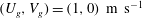
Figure 1. Profiles of the non-dimensional pressure variance in (a) the strongly convective boundary layer from
 $512^{3}$
LES using the Kosović model (dotted),
$512^{3}$
LES using the Kosović model (dotted),
 $1024^{3}$
LES using the Smagorinsky model (solid), the Kosović model (dash-dot) and
$1024^{3}$
LES using the Smagorinsky model (solid), the Kosović model (dash-dot) and
 $2048^{3}$
LES using the Kosović model (dashed), (b) a series of convective boundary layers from
$2048^{3}$
LES using the Kosović model (dashed), (b) a series of convective boundary layers from
 $512^{3}$
LES using the Kosović model (left to right:
$512^{3}$
LES using the Kosović model (left to right:
 $Q=0.24,0.06,0.12,0.20,0.16$
) and (c) the nearly neutral boundary layer from
$Q=0.24,0.06,0.12,0.20,0.16$
) and (c) the nearly neutral boundary layer from
 $1024^{3}$
LES using the Smagorinsky model (solid) and the Kosović model (dashed).
$1024^{3}$
LES using the Smagorinsky model (solid) and the Kosović model (dashed).
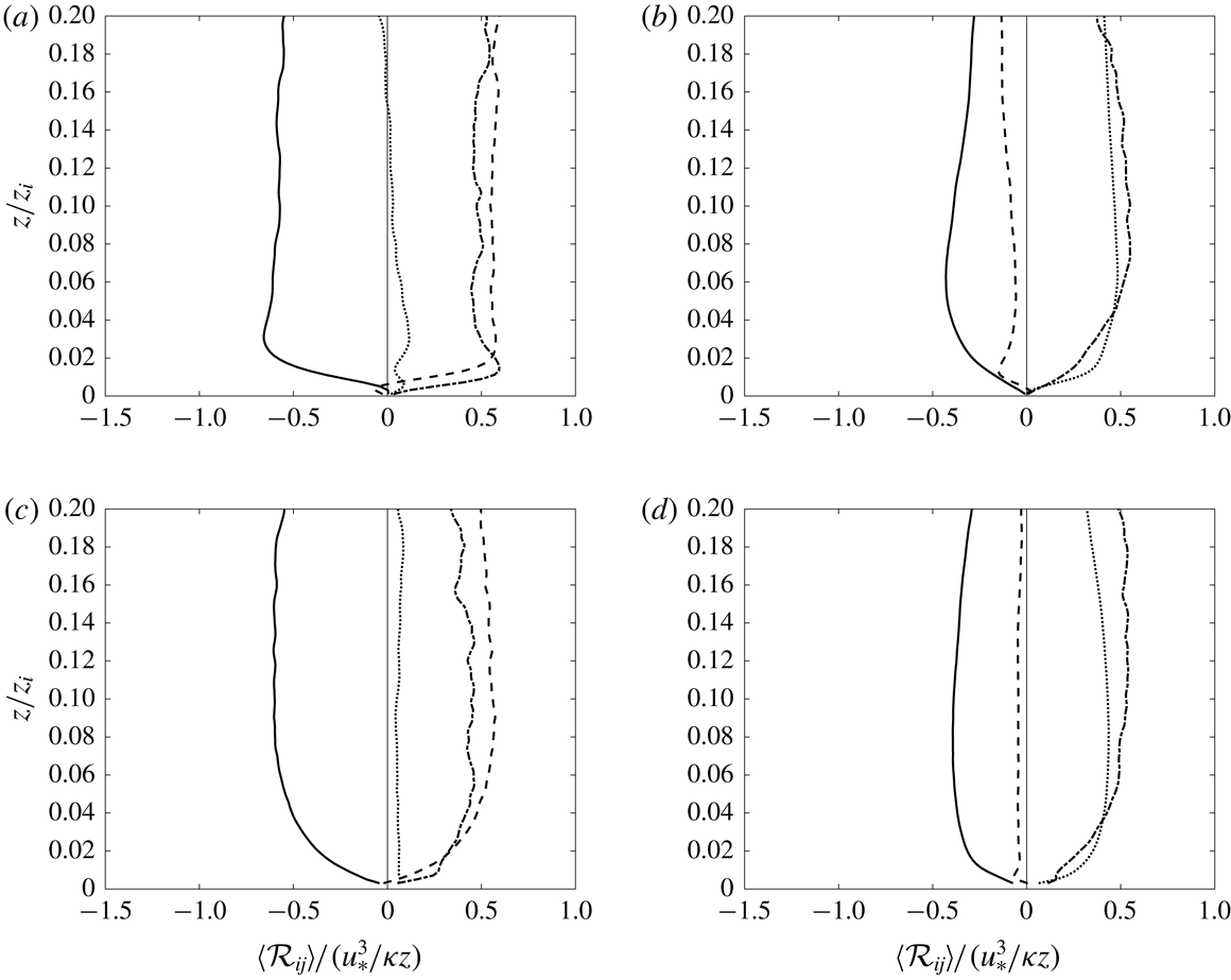
Figure 2. Profiles of the non-dimensional pressure–strain-rate correlation in the strongly convective boundary layer from LES using (a) the Smagorinsky model and (b) the Kosović model (
 $2048^{3}$
). The lines represent
$2048^{3}$
). The lines represent
 ${\mathcal{R}}_{11}$
(solid),
${\mathcal{R}}_{11}$
(solid),
 ${\mathcal{R}}_{22}$
(dotted) and
${\mathcal{R}}_{22}$
(dotted) and
 ${\mathcal{R}}_{33}$
(dashed). The LES resolution is
${\mathcal{R}}_{33}$
(dashed). The LES resolution is
 $1024^{3}$
here and hereafter unless otherwise noted. The predicted logarithmic profiles (3.2) agree well with the LES results for
$1024^{3}$
here and hereafter unless otherwise noted. The predicted logarithmic profiles (3.2) agree well with the LES results for
 $z/z_{i}=0.02$
.
$z/z_{i}=0.02$
.

Figure 3. Profiles of the pressure–strain-rate correlation in a series of convective boundary layers from 512
 $^{3}$
LES using the Kosović model: (a) dimensional (inside to outside:
$^{3}$
LES using the Kosović model: (a) dimensional (inside to outside:
 $Q=0.06,0.12,0.16,0.20,0.24$
); (b) non-dimensionalized using the mixed-layer scales. The lines represent
$Q=0.06,0.12,0.16,0.20,0.24$
); (b) non-dimensionalized using the mixed-layer scales. The lines represent
 ${\mathcal{R}}_{11}$
(solid),
${\mathcal{R}}_{11}$
(solid),
 ${\mathcal{R}}_{22}$
(dotted) and
${\mathcal{R}}_{22}$
(dotted) and
 ${\mathcal{R}}_{33}$
(dashed).
${\mathcal{R}}_{33}$
(dashed).

Figure 4. Profiles of the non-dimensional pressure–strain-rate correlation in the nearly neutral boundary layer from LES using (a) the Smagorinsky model and (b) the Kosović model. The lines represent
 ${\mathcal{R}}_{11}$
(solid),
${\mathcal{R}}_{11}$
(solid),
 ${\mathcal{R}}_{22}$
(dotted),
${\mathcal{R}}_{22}$
(dotted),
 ${\mathcal{R}}_{33}$
(dashed) and
${\mathcal{R}}_{33}$
(dashed) and
 ${\mathcal{R}}_{13}$
(dash-dot). Profiles with symbols were obtained using 512
${\mathcal{R}}_{13}$
(dash-dot). Profiles with symbols were obtained using 512
 $^{3}$
LES.
$^{3}$
LES.
3.1 Scaling properties
We first examine the scaling of the pressure–strain-rate correlation and the pressure fluctuations. The vertical profiles of the pressure variance,
 $\unicode[STIX]{x1D70E}_{p}^{2}$
, for several convective surface layers with different surface temperature flux values are shown in figure 1(a,b). The variance scales with
$\unicode[STIX]{x1D70E}_{p}^{2}$
, for several convective surface layers with different surface temperature flux values are shown in figure 1(a,b). The variance scales with
 $w_{\ast }^{4}$
, as expected. Figure 1(a) also compares results obtained from 512
$w_{\ast }^{4}$
, as expected. Figure 1(a) also compares results obtained from 512
 $^{3}$
, 1024
$^{3}$
, 1024
 $^{3}$
and 2048
$^{3}$
and 2048
 $^{3}$
LES. The differences among the different resolutions are relatively small, and are likely mainly due to the statistical uncertainties of the results. For the near neutral surface layer it appears to scale with
$^{3}$
LES. The differences among the different resolutions are relatively small, and are likely mainly due to the statistical uncertainties of the results. For the near neutral surface layer it appears to scale with
 $u_{\ast }^{4}$
(figure 1
c), also as expected. There appears to be only slight attenuation for
$u_{\ast }^{4}$
(figure 1
c), also as expected. There appears to be only slight attenuation for
 $z/z_{i}<0.02$
, consistent with the observation of Miles et al. (Reference Miles, Wyngaard and Otte2004) that the pressure variance near the surface is not significantly affected by the LES resolution, perhaps because pressure is a non-local variable. Figure 2 shows the vertical profile of the normal components of the pressure–strain-rate tensor,
$z/z_{i}<0.02$
, consistent with the observation of Miles et al. (Reference Miles, Wyngaard and Otte2004) that the pressure variance near the surface is not significantly affected by the LES resolution, perhaps because pressure is a non-local variable. Figure 2 shows the vertical profile of the normal components of the pressure–strain-rate tensor,
 ${\mathcal{R}}_{\unicode[STIX]{x1D6FC}\unicode[STIX]{x1D6FC}}$
(no summation for
${\mathcal{R}}_{\unicode[STIX]{x1D6FC}\unicode[STIX]{x1D6FC}}$
(no summation for
 $\unicode[STIX]{x1D6FC}$
), non-dimensionalized by
$\unicode[STIX]{x1D6FC}$
), non-dimensionalized by
 $w_{\ast }^{3}/z_{i}$
, obtained in the strongly convective boundary layer. (The LES resolution is
$w_{\ast }^{3}/z_{i}$
, obtained in the strongly convective boundary layer. (The LES resolution is
 $1024^{3}$
here and hereafter unless otherwise noted.) Consistent with the results obtained using the AHATS data (Nguyen et al.
Reference Nguyen, Horst, Oncley and Tong2013),
$1024^{3}$
here and hereafter unless otherwise noted.) Consistent with the results obtained using the AHATS data (Nguyen et al.
Reference Nguyen, Horst, Oncley and Tong2013),
 ${\mathcal{R}}_{11}$
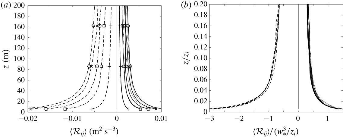
is positive, opposite to the results in a neutral boundary layer (see figure 4). The numerical values at
${\mathcal{R}}_{11}$
is positive, opposite to the results in a neutral boundary layer (see figure 4). The numerical values at
 $z/z_{i}=0.0069$
are within 25 % of the those obtained using AHATS data (Nguyen et al.
Reference Nguyen, Horst, Oncley and Tong2013). It decreases with increasing height, but appears to approach a constant value in the mixed layer. The magnitude is of order one, consistent with the mixed-layer scaling. To further examine the scaling property, we compute
$z/z_{i}=0.0069$
are within 25 % of the those obtained using AHATS data (Nguyen et al.
Reference Nguyen, Horst, Oncley and Tong2013). It decreases with increasing height, but appears to approach a constant value in the mixed layer. The magnitude is of order one, consistent with the mixed-layer scaling. To further examine the scaling property, we compute
 ${\mathcal{R}}_{\unicode[STIX]{x1D6FC}\unicode[STIX]{x1D6FC}}$
for essentially the same
${\mathcal{R}}_{\unicode[STIX]{x1D6FC}\unicode[STIX]{x1D6FC}}$
for essentially the same
 $z_{i}$
but a range of surface temperature flux (different
$z_{i}$
but a range of surface temperature flux (different
 $w_{\ast }$
) using a series of LES with
$w_{\ast }$
) using a series of LES with
 $512^{3}$
resolution (figure 3). The profiles, when scaled using the mixed-layer parameters (figure 3
b), essentially collapse, further indicating that
$512^{3}$
resolution (figure 3). The profiles, when scaled using the mixed-layer parameters (figure 3
b), essentially collapse, further indicating that
 ${\mathcal{R}}_{\unicode[STIX]{x1D6FC}\unicode[STIX]{x1D6FC}}$
has the mixed-layer scaling.
${\mathcal{R}}_{\unicode[STIX]{x1D6FC}\unicode[STIX]{x1D6FC}}$
has the mixed-layer scaling.
Figures 1 and 2 show some differences between the Smagorinsky and Kosović models. However, the results also show that the scaling properties are not sensitive to the model inaccuracies, providing further evidence that the scaling properties obtained are not affected by the model inaccuracies.
The increase of
 ${\mathcal{R}}_{\unicode[STIX]{x1D6FC}\unicode[STIX]{x1D6FC}}$
approaching the surface can be explained using Townsend’s attached-eddy model (Townsend Reference Townsend1976). He argued that eddies directly influenced by the presence of a wall are ‘attached’ to the wall. The large-scale motions near the wall can be considered as a superposition of the velocities of such eddies, which have different scales but similar velocity distributions. We extend the model to
${\mathcal{R}}_{\unicode[STIX]{x1D6FC}\unicode[STIX]{x1D6FC}}$
approaching the surface can be explained using Townsend’s attached-eddy model (Townsend Reference Townsend1976). He argued that eddies directly influenced by the presence of a wall are ‘attached’ to the wall. The large-scale motions near the wall can be considered as a superposition of the velocities of such eddies, which have different scales but similar velocity distributions. We extend the model to
 ${\mathcal{R}}_{\unicode[STIX]{x1D6FC}\unicode[STIX]{x1D6FC}}$
by considering it as a superposition of the contributions from attached convective eddies of different scales:
${\mathcal{R}}_{\unicode[STIX]{x1D6FC}\unicode[STIX]{x1D6FC}}$
by considering it as a superposition of the contributions from attached convective eddies of different scales:
 $$\begin{eqnarray}{\mathcal{R}}_{\unicode[STIX]{x1D6FC}\unicode[STIX]{x1D6FC}}(z)=\int _{z}^{z_{i}}N(z_{a})I_{\unicode[STIX]{x1D6FC}\unicode[STIX]{x1D6FC}}\left(\frac{z}{z_{a}}\right)\frac{\text{d}z_{a}}{z_{a}},\end{eqnarray}$$
where
 $z_{a}$
,
$z_{a}$
,
 $N(z_{a})$
, and
$N(z_{a})$
, and
 $I_{\unicode[STIX]{x1D6FC}\unicode[STIX]{x1D6FC}}$
are the centre location of the eddies of scale
$I_{\unicode[STIX]{x1D6FC}\unicode[STIX]{x1D6FC}}$
are the centre location of the eddies of scale
 $z_{a}$
, the intensity of the contributions and the functional form of the contributions from these eddies at height
$z_{a}$
, the intensity of the contributions and the functional form of the contributions from these eddies at height
 $z$
. Here
$z$
. Here
 $z_{a}$
is also the scale of the eddies centred at
$z_{a}$
is also the scale of the eddies centred at
 $z_{a}$
since the eddies are attached to the surface. For convective eddies
$z_{a}$
since the eddies are attached to the surface. For convective eddies
 $N=u_{f}^{3}/z_{a}$
, where
$N=u_{f}^{3}/z_{a}$
, where
 $u_{f}=(\unicode[STIX]{x1D6FD}Qz_{a})^{1/3}$
is the local-free-convection velocity scale (Wyngaard, Coté & Izumi Reference Wyngaard, Coté and Izumi1971). Here
$u_{f}=(\unicode[STIX]{x1D6FD}Qz_{a})^{1/3}$
is the local-free-convection velocity scale (Wyngaard, Coté & Izumi Reference Wyngaard, Coté and Izumi1971). Here
 $I_{\unicode[STIX]{x1D6FC}\unicode[STIX]{x1D6FC}}$
approaches a non-zero value near the wall since
$I_{\unicode[STIX]{x1D6FC}\unicode[STIX]{x1D6FC}}$
approaches a non-zero value near the wall since
 $p$
and
$p$
and
 $s_{\unicode[STIX]{x1D6FC}\unicode[STIX]{x1D6FC}}$
are non-zero. The integral in (3.1) leads to
$s_{\unicode[STIX]{x1D6FC}\unicode[STIX]{x1D6FC}}$
are non-zero. The integral in (3.1) leads to
 $$\begin{eqnarray}{\mathcal{R}}_{\unicode[STIX]{x1D6FC}\unicode[STIX]{x1D6FC}}=\unicode[STIX]{x1D6FD}Q\left[c_{1}+c_{2}\log \frac{z_{i}}{z}\right],\end{eqnarray}$$
where
 $c_{1}$
and
$c_{1}$
and
 $c_{2}$
are coefficients that are independent of the flow parameters, which are determined here by plotting the
$c_{2}$
are coefficients that are independent of the flow parameters, which are determined here by plotting the
 ${\mathcal{R}}_{\unicode[STIX]{x1D6FC}\unicode[STIX]{x1D6FC}}$
profiles in the linear–log scales and fitting a straight line to the logarithmic portion. The predicted logarithmic behaviour is consistent with the
${\mathcal{R}}_{\unicode[STIX]{x1D6FC}\unicode[STIX]{x1D6FC}}$
profiles in the linear–log scales and fitting a straight line to the logarithmic portion. The predicted logarithmic behaviour is consistent with the
 ${\mathcal{R}}_{\unicode[STIX]{x1D6FC}\unicode[STIX]{x1D6FC}}$
profiles shown in figure 2. These results show that the pressure–strain-rate correlation in the strongly convective surface layer is almost unaffected by the near-wall resolution, at least for the resolutions used in the present study.
${\mathcal{R}}_{\unicode[STIX]{x1D6FC}\unicode[STIX]{x1D6FC}}$
profiles shown in figure 2. These results show that the pressure–strain-rate correlation in the strongly convective surface layer is almost unaffected by the near-wall resolution, at least for the resolutions used in the present study.
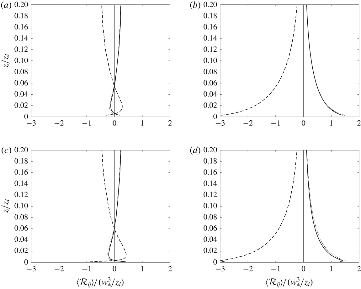
Figure 4 shows the vertical profile of
 ${\mathcal{R}}_{ij}$
, non-dimensionalized by
${\mathcal{R}}_{ij}$
, non-dimensionalized by
 $u_{\ast }^{3}/z$
, obtained using the LES fields of the near neutral boundary layer. Between 30 and 70 m (
$u_{\ast }^{3}/z$
, obtained using the LES fields of the near neutral boundary layer. Between 30 and 70 m (
 $z/z_{i}=0.03{-}0.07$
), they have relatively constant values, with
$z/z_{i}=0.03{-}0.07$
), they have relatively constant values, with
 ${\mathcal{R}}_{11}$
being negative and
${\mathcal{R}}_{11}$
being negative and
 ${\mathcal{R}}_{22}$
and
${\mathcal{R}}_{22}$
and
 ${\mathcal{R}}_{33}$
being positive, consistent with the surface-layer scaling and its role of causing return to isotropy. The decrease (the departure from the expected surface-layer scaling) below
${\mathcal{R}}_{33}$
being positive, consistent with the surface-layer scaling and its role of causing return to isotropy. The decrease (the departure from the expected surface-layer scaling) below
 $z/z_{i}=0.03$
(the 15th grid point) is due to the under-resolution of the strain rate by LES, since the pressure fluctuations are not significantly under-resolved (figure 1
c) (also see the results for the pressure–strain-rate cospectra for more details). At the tenth grid point, approximately 80 % of the pressure–strain-rate correlation is resolved compared to the highest values, e.g.
$z/z_{i}=0.03$
(the 15th grid point) is due to the under-resolution of the strain rate by LES, since the pressure fluctuations are not significantly under-resolved (figure 1
c) (also see the results for the pressure–strain-rate cospectra for more details). At the tenth grid point, approximately 80 % of the pressure–strain-rate correlation is resolved compared to the highest values, e.g.
 ${\mathcal{R}}_{11}$
at
${\mathcal{R}}_{11}$
at
 $z/z_{i}=0.02$
and
$z/z_{i}=0.02$
and
 $0.06$
have values of approximate 0.8, and 1.0 respectively, the latter being considered well resolved. The extent of resolution is similar to the vertical velocity variance. The results for the 512
$0.06$
have values of approximate 0.8, and 1.0 respectively, the latter being considered well resolved. The extent of resolution is similar to the vertical velocity variance. The results for the 512
 $^{3}$
LES show a similar trend, again with the pressure–strain-rate correlation well resolved at the 15th grid point. The off-diagonal component
$^{3}$
LES show a similar trend, again with the pressure–strain-rate correlation well resolved at the 15th grid point. The off-diagonal component
 ${\mathcal{R}}_{13}$
is positive, also consistent with return to isotropy (the shear stress is negative).
${\mathcal{R}}_{13}$
is positive, also consistent with return to isotropy (the shear stress is negative).
The pressure–strain-rate correlation profiles for the moderately convective surface layer (figure 5) for
 $-z/L>1$
have similar trends to the strongly convective surface layer. They are similar to the neutral surface layer for small
$-z/L>1$
have similar trends to the strongly convective surface layer. They are similar to the neutral surface layer for small
 $-z/L$
values (
$-z/L$
values (
 ${<}0.5{-}0.7$
), with
${<}0.5{-}0.7$
), with
 ${\mathcal{R}}_{11}$
being negative. However,
${\mathcal{R}}_{11}$
being negative. However,
 ${\mathcal{R}}_{33}$
is moving toward positive values as
${\mathcal{R}}_{33}$
is moving toward positive values as
 $z$
decreases but still has not crossed the zero value, likely due to the under-resolution near the surface. Similar to the near neutral surface layer,
$z$
decreases but still has not crossed the zero value, likely due to the under-resolution near the surface. Similar to the near neutral surface layer,
 ${\mathcal{R}}_{13}$
is also positive (not shown). These results suggest that the pressure–strain-rate correlation contains multiple scales.
${\mathcal{R}}_{13}$
is also positive (not shown). These results suggest that the pressure–strain-rate correlation contains multiple scales.

Figure 5. Profiles of the non-dimensional pressure–strain-rate correlation in the moderately convective boundary layer from LES using (a) the Smagorinsky model and (b) the Kosović model (
 $2048^{3}$
). The lines represent
$2048^{3}$
). The lines represent
 ${\mathcal{R}}_{11}$
(solid),
${\mathcal{R}}_{11}$
(solid),
 ${\mathcal{R}}_{22}$
(dotted) and
${\mathcal{R}}_{22}$
(dotted) and
 ${\mathcal{R}}_{33}$
(dashed).
${\mathcal{R}}_{33}$
(dashed).

Figure 6. Pressure spectrum in the strongly convective boundary layer from LES using (a) the Smagorinsky model and (b) the Kosović model (
 $2048^{3}$
), non-dimensionalized by
$2048^{3}$
), non-dimensionalized by
 $C_{p}=w_{\ast }^{2}(\unicode[STIX]{x1D705}\unicode[STIX]{x1D6FD}Q)^{2/3}z_{i}^{5/3}$
(see § 3.2 for details). The lines represent heights of 16 m (solid), 20 m (dashed) and 30 m (dotted).
$C_{p}=w_{\ast }^{2}(\unicode[STIX]{x1D705}\unicode[STIX]{x1D6FD}Q)^{2/3}z_{i}^{5/3}$
(see § 3.2 for details). The lines represent heights of 16 m (solid), 20 m (dashed) and 30 m (dotted).

Figure 7. Pressure spectrum in a series of convective boundary layers at 16 m from 512
 $^{3}$
LES using the Kosović model: (a) dimensional; (b) non-dimensionalized by
$^{3}$
LES using the Kosović model: (a) dimensional; (b) non-dimensionalized by
 $C_{p}=w_{\ast }^{2}(\unicode[STIX]{x1D705}\unicode[STIX]{x1D6FD}Q)^{2/3}z_{i}^{5/3}$
.
$C_{p}=w_{\ast }^{2}(\unicode[STIX]{x1D705}\unicode[STIX]{x1D6FD}Q)^{2/3}z_{i}^{5/3}$
.

Figure 8. Pressure spectrum in the nearly neutral surface layer from LES using the Smagorinsky model, non-dimensionalized by
 $C_{p}=u_{\ast }^{4}z_{i}$
. The lines represent 16 m (solid), 20 m (dashed) and 30 m (dotted).
$C_{p}=u_{\ast }^{4}z_{i}$
. The lines represent 16 m (solid), 20 m (dashed) and 30 m (dotted).
3.2 Spectral characteristics
To examine the contributions to
 ${\mathcal{R}}_{ij}$
from the different length scales, we investigate the pressure spectrum and the pressure–strain-rate cospectra at scales greater than
${\mathcal{R}}_{ij}$
from the different length scales, we investigate the pressure spectrum and the pressure–strain-rate cospectra at scales greater than
 $z$
(
$z$
(
 $kz<1$
). The pressure spectrum in the convective surface layer (figure 6) has a scaling exponent close to
$kz<1$
). The pressure spectrum in the convective surface layer (figure 6) has a scaling exponent close to
 $-5/3$
. If we use the parameters for a free-convective surface layer, the buoyancy parameter
$-5/3$
. If we use the parameters for a free-convective surface layer, the buoyancy parameter
 $\unicode[STIX]{x1D6FD}$
, the surface temperature flux
$\unicode[STIX]{x1D6FD}$
, the surface temperature flux
 $Q$
, and the wavenumber
$Q$
, and the wavenumber
 $k$
, the pressure spectrum for
$k$
, the pressure spectrum for
 $kz\ll 1$
is predicted as
$kz\ll 1$
is predicted as
 $$\begin{eqnarray}\unicode[STIX]{x1D719}_{p}(k)=(\unicode[STIX]{x1D6FD}Q)^{4/3}k^{-7/3}.\end{eqnarray}$$
The predicted scaling exponent is inconsistent with the LES results, suggesting that the spectrum cannot be determined entirely by the surface-layer parameters. Figure 7 shows that the pressure spectra obtained using the series of
 $512^{3}$
LES of convective surface layers collapse when scaled using a combination of mixed-layer and surface-layer scales. This scaling will be further discussed in § 3.3. For the neutral ABL, the prediction using the surface-layer parameters is
$512^{3}$
LES of convective surface layers collapse when scaled using a combination of mixed-layer and surface-layer scales. This scaling will be further discussed in § 3.3. For the neutral ABL, the prediction using the surface-layer parameters is
 $$\begin{eqnarray}\unicode[STIX]{x1D719}_{p}(k)=u_{\ast }^{4}k^{-1},\end{eqnarray}$$
which is consistent with the results shown in figure 8.
We now predict the scaling exponents of the pressure–strain-rate cospectra for different
 $-z/L$
ranges. For
$-z/L$
ranges. For
 $kz\ll 1$
in a free convective surface layer, using the parameters
$kz\ll 1$
in a free convective surface layer, using the parameters
 $\unicode[STIX]{x1D6FD}$
,
$\unicode[STIX]{x1D6FD}$
,
 $Q$
and
$Q$
and
 $k$
, the cospectra are predicted to have the form
$k$
, the cospectra are predicted to have the form
 $$\begin{eqnarray}C_{\unicode[STIX]{x1D6FC}\unicode[STIX]{x1D6FC}}^{\prime }(k)=\unicode[STIX]{x1D6FD}Qk^{-1}.\end{eqnarray}$$
Interestingly, equation (3.5) can also be written as
 $$\begin{eqnarray}kC_{\unicode[STIX]{x1D6FC}\unicode[STIX]{x1D6FC}}^{\prime }(k)=\unicode[STIX]{x1D6FD}Q\sim u_{f}^{3}k.\end{eqnarray}$$
This expression suggests that the pressure–strain-rate correlation at wavenumber
 $k$
is determined by the convective eddies of scale
$k$
is determined by the convective eddies of scale
 $1/k$
. In § 3.2 we will address the fact that the scaling exponent of pressure spectrum in the strongly convective surface layers is not consistent with the prediction using the free-convection parameters but the pressure–strain-rate cospectra are.
$1/k$
. In § 3.2 we will address the fact that the scaling exponent of pressure spectrum in the strongly convective surface layers is not consistent with the prediction using the free-convection parameters but the pressure–strain-rate cospectra are.
For the near neutral surface layer, the parameters are
 $u_{\ast }$
and
$u_{\ast }$
and
 $k$
, resulting in a cospectrum of the form
$k$
, resulting in a cospectrum of the form
 $$\begin{eqnarray}C_{\unicode[STIX]{x1D6FC}\unicode[STIX]{x1D6FC}}^{\prime }(k)=u_{\ast }^{3}.\end{eqnarray}$$
Thus the cospectra are independent of
 $k$
.
$k$
.
For the moderately convective surface layer, the cospectra for
 $-z/L>1$
(termed the convective layer in Tong & Nguyen (Reference Tong and Nguyen2015)) are similar to those in the convective surface layer. For
$-z/L>1$
(termed the convective layer in Tong & Nguyen (Reference Tong and Nguyen2015)) are similar to those in the convective surface layer. For
 $-z/L<1$
(the convective–dynamic layer), using the multi-point Monin–Obukhov similarity (MMO) (Tong & Nguyen Reference Tong and Nguyen2015) we predict that for
$-z/L<1$
(the convective–dynamic layer), using the multi-point Monin–Obukhov similarity (MMO) (Tong & Nguyen Reference Tong and Nguyen2015) we predict that for
 $-kL<1$
(the convective range), they are similar to those in the convective surface layer. For
$-kL<1$
(the convective range), they are similar to those in the convective surface layer. For
 $-kL>1$
(the dynamic range) they are similar to those in the neutral surface layer. However, the signs of the cospectra can be different for the two ranges. The qualitatively different behaviours of the cospectra in the different scaling ranges suggest that the pressure–strain-rate correlation contains multiple scales that correspond to different physical processes.
$-kL>1$
(the dynamic range) they are similar to those in the neutral surface layer. However, the signs of the cospectra can be different for the two ranges. The qualitatively different behaviours of the cospectra in the different scaling ranges suggest that the pressure–strain-rate correlation contains multiple scales that correspond to different physical processes.
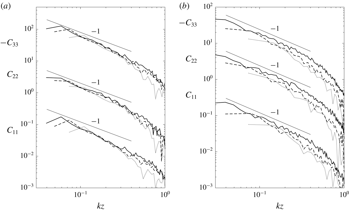
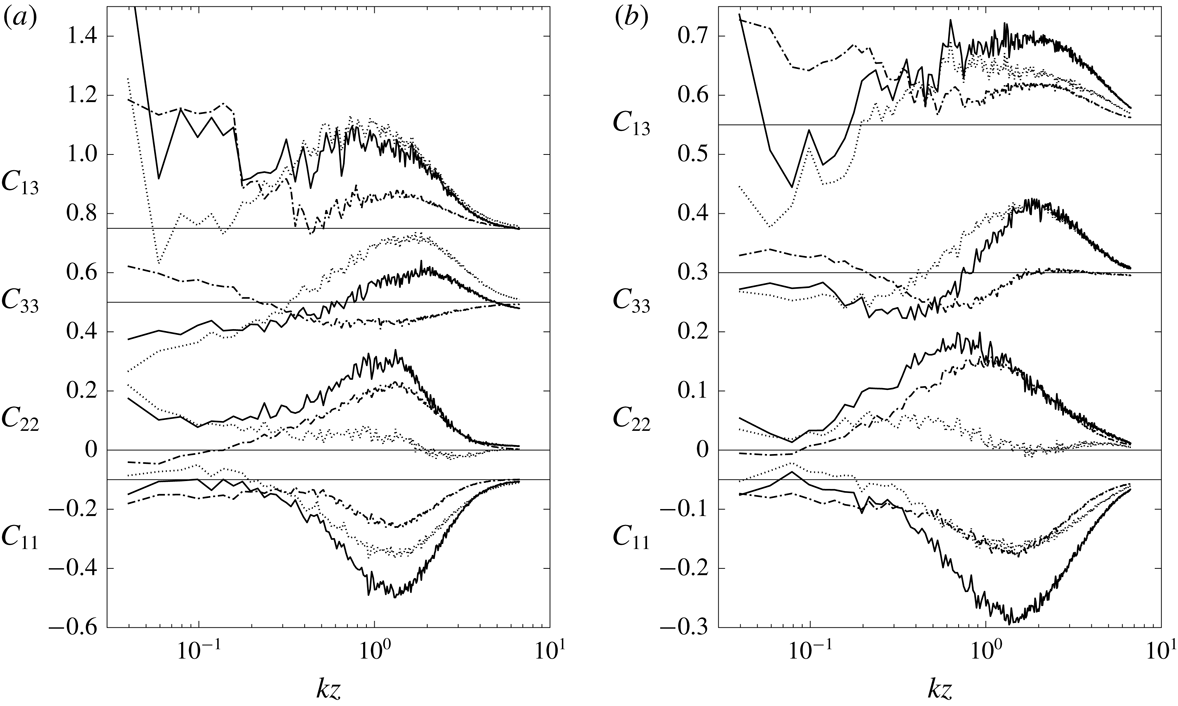
The pressure–strain-rate cospectra for the strongly convective surface layer at several different heights from the surface are shown in figure 9. The non-dimensional cospectra largely collapse in the scaling range with a
 $k^{-1}$
scaling exponent, consistent with our prediction (3.5). The cospectra obtained using the 1024
$k^{-1}$
scaling exponent, consistent with our prediction (3.5). The cospectra obtained using the 1024
 $^{3}$
and 2048
$^{3}$
and 2048
 $^{3}$
LES are essentially identical, indicating that they are well resolved and are insensitive to the resolution. They peak near
$^{3}$
LES are essentially identical, indicating that they are well resolved and are insensitive to the resolution. They peak near
 $kz_{i}=1$
, indicating that the eddies of scales from
$kz_{i}=1$
, indicating that the eddies of scales from
 $z$
to
$z$
to
 $z_{i}$
have similar contributions to
$z_{i}$
have similar contributions to
 ${\mathcal{R}}_{\unicode[STIX]{x1D6FC}\unicode[STIX]{x1D6FC}}$
, resulting in the logarithmic profile (figure 4). Therefore in this case the pressure–strain-rate correlation has the same scaling as the horizontal velocity variances.
${\mathcal{R}}_{\unicode[STIX]{x1D6FC}\unicode[STIX]{x1D6FC}}$
, resulting in the logarithmic profile (figure 4). Therefore in this case the pressure–strain-rate correlation has the same scaling as the horizontal velocity variances.

Figure 9. Pressure–strain-rate cospectra in the strongly convective boundary layer from LES using (a) the Smagorinsky model and (b) the Kosović model (
 $2048^{3}$
). The lines represent heights of (a) 16 m (solid), 20 m (dashed) and 30 m (dotted), (b) 8 m (solid), 16 m (dashed) and 30 m (dotted). Here
$2048^{3}$
). The lines represent heights of (a) 16 m (solid), 20 m (dashed) and 30 m (dotted), (b) 8 m (solid), 16 m (dashed) and 30 m (dotted). Here
 $C_{\unicode[STIX]{x1D6FC}\unicode[STIX]{x1D6FC}}=C_{\unicode[STIX]{x1D6FC}\unicode[STIX]{x1D6FC}}^{\prime }/(w_{\ast }^{3}z/z_{i})$
. For clarity,
$C_{\unicode[STIX]{x1D6FC}\unicode[STIX]{x1D6FC}}=C_{\unicode[STIX]{x1D6FC}\unicode[STIX]{x1D6FC}}^{\prime }/(w_{\ast }^{3}z/z_{i})$
. For clarity,
 $C_{11}$
has been multiplied by 0.05 in (a) and (b), and
$C_{11}$
has been multiplied by 0.05 in (a) and (b), and
 $C_{33}$
has been multiplied by 20 in (a) and 5 in (b).
$C_{33}$
has been multiplied by 20 in (a) and 5 in (b).

Figure 10. Pressure–strain-rate cospectra in the nearly neutral surface layer from LES using (a) the Smagorinsky model and (b) the Kosović model. The lines represent heights of 16 m (solid), 20 m (dashed) and 30 m (dotted). Here
 $C_{\unicode[STIX]{x1D6FC}\unicode[STIX]{x1D6FC}}=C_{\unicode[STIX]{x1D6FC}\unicode[STIX]{x1D6FC}}^{\prime }/u_{\ast }^{3}$
. For clarity, some of the cospectra have been shifted vertically. Each horizontal line represents the zero value for the corresponding cospectrum.
$C_{\unicode[STIX]{x1D6FC}\unicode[STIX]{x1D6FC}}=C_{\unicode[STIX]{x1D6FC}\unicode[STIX]{x1D6FC}}^{\prime }/u_{\ast }^{3}$
. For clarity, some of the cospectra have been shifted vertically. Each horizontal line represents the zero value for the corresponding cospectrum.
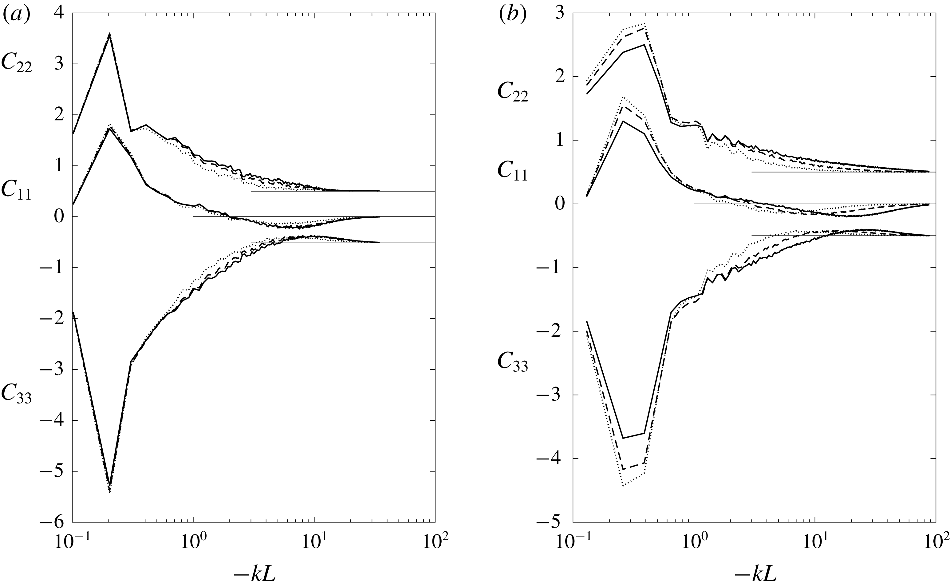
Figure 11. Pressure–strain-rate cospectra in the moderately convective surface layer from LES using (a) the Smagorinsky model and (b) the Kosović model (
 $2048^{3}$
). The lines represent heights of (a) 16 m (solid), 20 m (dashed) and 30 m (dotted), (b) 8 m (solid), 16 m (dashed) and 30 m (dotted). Here
$2048^{3}$
). The lines represent heights of (a) 16 m (solid), 20 m (dashed) and 30 m (dotted), (b) 8 m (solid), 16 m (dashed) and 30 m (dotted). Here
 $C_{\unicode[STIX]{x1D6FC}\unicode[STIX]{x1D6FC}}=C_{\unicode[STIX]{x1D6FC}\unicode[STIX]{x1D6FC}}^{\prime }/u_{\ast }^{3}$
. For clarity, some of the cospectra have been shifted vertically.
$C_{\unicode[STIX]{x1D6FC}\unicode[STIX]{x1D6FC}}=C_{\unicode[STIX]{x1D6FC}\unicode[STIX]{x1D6FC}}^{\prime }/u_{\ast }^{3}$
. For clarity, some of the cospectra have been shifted vertically.
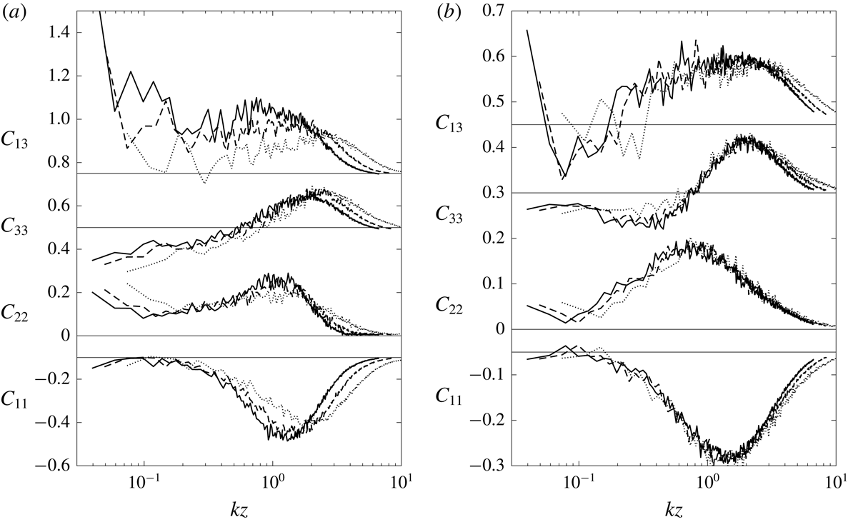
It is interesting to compare these cospectra with those in a neutral boundary layer (figure 10), where
 ${\mathcal{R}}_{11}$
is negative. Near
${\mathcal{R}}_{11}$
is negative. Near
 $kz=1$
,
$kz=1$
,
 $C_{11}$
is negative while
$C_{11}$
is negative while
 $C_{22}$
and
$C_{22}$
and
 $C_{33}$
are positive, indicating return to isotropy due to the shear production of the
$C_{33}$
are positive, indicating return to isotropy due to the shear production of the
 $u$
fluctuations. For
$u$
fluctuations. For
 $kz\ll 1$
,
$kz\ll 1$
,
 $C_{33}$
becomes negative and
$C_{33}$
becomes negative and
 $C_{22}$
is still positive, indicating redistribution of energy from the
$C_{22}$
is still positive, indicating redistribution of energy from the
 $w$
to the
$w$
to the
 $v$
component. Interestingly,
$v$
component. Interestingly,
 $C_{11}$
now has very small magnitudes (although still negative), indicating that the
$C_{11}$
now has very small magnitudes (although still negative), indicating that the
 $u$
component does not exchange significant amounts of energy with the other components, likely because the
$u$
component does not exchange significant amounts of energy with the other components, likely because the
 $u$
component is still receiving energy from the production associated with the large eddies, although at a very small rate, estimated as
$u$
component is still receiving energy from the production associated with the large eddies, although at a very small rate, estimated as
 $u_{\ast }^{2}kz\unicode[STIX]{x2202}U/\unicode[STIX]{x2202}z\sim u_{\ast }^{3}k$
. These results are consistent with the attached-eddy model of Townsend and the ‘inactive motion’ description of Bradshaw (Reference Bradshaw1967). These eddies are produced at the height
$u_{\ast }^{2}kz\unicode[STIX]{x2202}U/\unicode[STIX]{x2202}z\sim u_{\ast }^{3}k$
. These results are consistent with the attached-eddy model of Townsend and the ‘inactive motion’ description of Bradshaw (Reference Bradshaw1967). These eddies are produced at the height
 $z\sim 1/k$
by the mean shear there. Their energy is then transported toward the surface by irrotational pressure fluctuations, and redistributed from the
$z\sim 1/k$
by the mean shear there. Their energy is then transported toward the surface by irrotational pressure fluctuations, and redistributed from the
 $w$
to
$w$
to
 $v$
component. This redistribution of energy is in some way similar to that in a convective surface layer. However, in a convective surface layer, the large convective eddies are much more energetic than the large neutral eddies (
$v$
component. This redistribution of energy is in some way similar to that in a convective surface layer. However, in a convective surface layer, the large convective eddies are much more energetic than the large neutral eddies (
 $u_{f}$
versus
$u_{f}$
versus
 $u_{\ast }$
), thereby reversing the sign of
$u_{\ast }$
), thereby reversing the sign of
 $C_{11}$
. Since
$C_{11}$
. Since
 ${\mathcal{R}}_{13}$
is positive
${\mathcal{R}}_{13}$
is positive
 $C_{13}$
is also positive and peaks near
$C_{13}$
is also positive and peaks near
 $kz=1$
, as expected. In all cases, the peaks of the cospectra are quite well resolved.
$kz=1$
, as expected. In all cases, the peaks of the cospectra are quite well resolved.
The cospectra for the moderately convective surface layer at three heights from the surface are shown in figure 11. According to MMO, in this surface layer
 $L$
is also an important horizontal length scale. Thus we use
$L$
is also an important horizontal length scale. Thus we use
 $-kL$
as the non-dimensional wavenumber. Near
$-kL$
as the non-dimensional wavenumber. Near
 $kz=3$
(equivalent to
$kz=3$
(equivalent to
 $-kL\approx 20$
at
$-kL\approx 20$
at
 $z=16~\text{m}$
),
$z=16~\text{m}$
),
 $C_{11}$
is negative while
$C_{11}$
is negative while
 $C_{22}$
and
$C_{22}$
and
 $C_{33}$
are positive, consistent with return to isotropy. For
$C_{33}$
are positive, consistent with return to isotropy. For
 $-kL<1$
,
$-kL<1$
,
 $C_{33}$
is negative while
$C_{33}$
is negative while
 $C_{22}$
and
$C_{22}$
and
 $C_{11}$
are positive, resulting in anisotropy. Thus, there are two distinct redistribution processes, one at scales of order
$C_{11}$
are positive, resulting in anisotropy. Thus, there are two distinct redistribution processes, one at scales of order
 $z$
and one beyond
$z$
and one beyond
 $-L$
. The cospectra largely collapse for
$-L$
. The cospectra largely collapse for
 $-kL<1$
when scaled using
$-kL<1$
when scaled using
 $-L$
. The scaling for
$-L$
. The scaling for
 $C_{22}$
and
$C_{22}$
and
 $C_{33}$
is consistent with
$C_{33}$
is consistent with
 $k^{-1}$
(not shown). For
$k^{-1}$
(not shown). For
 $C_{11}$
the scaling exponent is greater than
$C_{11}$
the scaling exponent is greater than
 $-1$
, perhaps related to the change of sign at a smaller
$-1$
, perhaps related to the change of sign at a smaller
 $-kL$
values and thus the smaller scaling range. According to MMO, there should also be a scaling range between
$-kL$
values and thus the smaller scaling range. According to MMO, there should also be a scaling range between
 $-kL>1$
and
$-kL>1$
and
 $kz<1$
. However, this scaling range may require a very large separation of scales (
$kz<1$
. However, this scaling range may require a very large separation of scales (
 $z$
,
$z$
,
 $-L$
and
$-L$
and
 $z_{i}$
), as suggested by the results for the neutral surface layer. Due to the limited scale separation (
$z_{i}$
), as suggested by the results for the neutral surface layer. Due to the limited scale separation (
 $-L$
and
$-L$
and
 $z_{i}$
) for the ABL simulated, the scaling range is not observed here. The sign change from
$z_{i}$
) for the ABL simulated, the scaling range is not observed here. The sign change from
 $kz\sim 1$
to
$kz\sim 1$
to
 $-kL<1$
and the collapse of the cospectra indicate that
$-kL<1$
and the collapse of the cospectra indicate that
 $L$
is indeed a key horizontal length scale. MMO assumes that it is imposed on the horizontal motions by the pressure–strain-rate correlation. The results in the present study therefore provide important support to MMO.
$L$
is indeed a key horizontal length scale. MMO assumes that it is imposed on the horizontal motions by the pressure–strain-rate correlation. The results in the present study therefore provide important support to MMO.
3.3 Further discussions on the scaling properties
As mentioned in the Introduction, previous studies (e.g. Wyngaard et al.
Reference Wyngaard, Coté and Izumi1971) have suggested that the
 ${\mathcal{R}}_{ij}$
has the surface-layer scaling, which is inconsistent with the mixed-layer scaling of the horizontal velocity variances. To explain this apparent contradiction, we consider the surface-layer similarity in terms of MMO, according to which, turbulent statistics in the wavenumber space depend on the similarity variables
${\mathcal{R}}_{ij}$
has the surface-layer scaling, which is inconsistent with the mixed-layer scaling of the horizontal velocity variances. To explain this apparent contradiction, we consider the surface-layer similarity in terms of MMO, according to which, turbulent statistics in the wavenumber space depend on the similarity variables
 $kL$
and
$kL$
and
 $z/L$
. Since the pressure–strain-rate cospectra and the horizontal velocity spectra both follow MMO as shown above and in Tong & Nguyen (Reference Tong and Nguyen2015), there is no inconsistency in spectral scaling. The inconsistency arises when the velocity variances and the pressure–strain-rate correlation, which are the integrated velocity spectra and the pressure–strain-rate cospectra, are considered in term of the (original) Monin–Obukhov similarity. We examine this issue in the following.
$z/L$
. Since the pressure–strain-rate cospectra and the horizontal velocity spectra both follow MMO as shown above and in Tong & Nguyen (Reference Tong and Nguyen2015), there is no inconsistency in spectral scaling. The inconsistency arises when the velocity variances and the pressure–strain-rate correlation, which are the integrated velocity spectra and the pressure–strain-rate cospectra, are considered in term of the (original) Monin–Obukhov similarity. We examine this issue in the following.
The similarity properties of the pressure–strain-rate correlation and the horizontal velocity variances can be obtained from the MMO scaling properties of the pressure–strain-rate cospectra and the velocity spectra. For
 $-z/L\gg 1$
, at the horizontal scales of order
$-z/L\gg 1$
, at the horizontal scales of order
 $z_{i}$
and
$z_{i}$
and
 $z$
, the pressure–strain-rate cospectra scale as
$z$
, the pressure–strain-rate cospectra scale as
 $w_{\ast }^{3}/z_{i}$
and
$w_{\ast }^{3}/z_{i}$
and
 $u_{f}^{3}/z$
respectively, which are effectively the same scale. In the meantime, the horizontal velocity variances,
$u_{f}^{3}/z$
respectively, which are effectively the same scale. In the meantime, the horizontal velocity variances,
 $\unicode[STIX]{x1D70E}_{h}^{2}$
, are dominated by the
$\unicode[STIX]{x1D70E}_{h}^{2}$
, are dominated by the
 $z_{i}$
scales. Therefore, the pressure–strain-rate correlation actually has the same scaling as
$z_{i}$
scales. Therefore, the pressure–strain-rate correlation actually has the same scaling as
 $\unicode[STIX]{x1D70E}_{h}^{2}$
. For
$\unicode[STIX]{x1D70E}_{h}^{2}$
. For
 $-z/L$
values of order one, the pressure–strain-rate correlation contains both the mixed-layer scales and the surface-layer scales. Here we provide an explanation for the apparent surface-layer scaling (
$-z/L$
values of order one, the pressure–strain-rate correlation contains both the mixed-layer scales and the surface-layer scales. Here we provide an explanation for the apparent surface-layer scaling (
 $z$
and
$z$
and
 $u_{\ast }$
) by hypothesizing that the pressure–strain-rate correlation consists of the neutral and convective contributions,
$u_{\ast }$
) by hypothesizing that the pressure–strain-rate correlation consists of the neutral and convective contributions,
 $u_{f}^{3}/zf(z/z_{i})$
and
$u_{f}^{3}/zf(z/z_{i})$
and
 $u_{\ast }^{3}/z\unicode[STIX]{x1D719}_{s}(z/L)$
respectively, where a dimensionless function
$u_{\ast }^{3}/z\unicode[STIX]{x1D719}_{s}(z/L)$
respectively, where a dimensionless function
 $\unicode[STIX]{x1D719}_{s}$
is included to represent the effects of convective eddies (e.g. altering the mean shear) on the neutral contribution. The normal components of the pressure–strain-rate correlation therefore can be (symbolically) estimated as
$\unicode[STIX]{x1D719}_{s}$
is included to represent the effects of convective eddies (e.g. altering the mean shear) on the neutral contribution. The normal components of the pressure–strain-rate correlation therefore can be (symbolically) estimated as
 $$\begin{eqnarray}\frac{w_{\ast }^{3}}{z_{i}}f(z/z_{i})+\frac{u_{\ast }^{3}}{z}\unicode[STIX]{x1D719}_{s}(z/L)=\frac{u_{\ast }^{3}}{z}\left\{\frac{w_{\ast }^{3}}{u_{\ast }^{3}}\frac{z}{z_{i}}f(z/z_{i})+\unicode[STIX]{x1D719}_{s}(z/L)\right\}=\frac{u_{\ast }^{3}}{z}\left\{-\frac{z}{\unicode[STIX]{x1D705}L}f(z/z_{i})+\unicode[STIX]{x1D719}_{s}(z/L)\right\}.\end{eqnarray}$$
We have absorbed the coefficients for the terms into the non-dimensional function
 $f$
and
$f$
and
 $\unicode[STIX]{x1D719}_{s}$
. The function
$\unicode[STIX]{x1D719}_{s}$
. The function
 $f(z/z_{i})$
varies slowly (e.g. logarithmically as suggested by (3.2)) as
$f(z/z_{i})$
varies slowly (e.g. logarithmically as suggested by (3.2)) as
 $z/z_{i}\rightarrow 0$
; therefore so does the convective contribution, leading to the apparent scaling of
$z/z_{i}\rightarrow 0$
; therefore so does the convective contribution, leading to the apparent scaling of
 ${\mathcal{R}}_{\unicode[STIX]{x1D6FC}\unicode[STIX]{x1D6FC}}$
with
${\mathcal{R}}_{\unicode[STIX]{x1D6FC}\unicode[STIX]{x1D6FC}}$
with
 $z/L$
. We emphasize that this apparent surface-layer scaling does not require the convective contribution to be small, only that it varies slowly near the surface. However, equation (3.2) suggests that
$z/L$
. We emphasize that this apparent surface-layer scaling does not require the convective contribution to be small, only that it varies slowly near the surface. However, equation (3.2) suggests that
 $z_{i}/L$
influences the value of
$z_{i}/L$
influences the value of
 $f(L/z_{i})$
. Therefore, different
$f(L/z_{i})$
. Therefore, different
 $z_{i}/L$
values will lead to scatters in the similarity function obtained in the surface layer.
$z_{i}/L$
values will lead to scatters in the similarity function obtained in the surface layer.
The above discussions suggest that the budget equations of
 $\unicode[STIX]{x1D70E}_{h}^{2}$
also have both the surface-layer and mixed-layer contributions with the latter leading to the mixed-layer scaling of
$\unicode[STIX]{x1D70E}_{h}^{2}$
also have both the surface-layer and mixed-layer contributions with the latter leading to the mixed-layer scaling of
 $\unicode[STIX]{x1D70E}_{h}^{2}$
. Therefore, the apparent inconsistency between the scaling properties of the velocity variances and their budgets is a result of the multi-scale nature of the surface layer. The horizontal velocity variances are dominated by the mixed-layer contributions; however, their time rate of changes can be contain significant surface-layer contributions or even be dominated by them. As pointed out by Tong & Nguyen (Reference Tong and Nguyen2015), according to MMO, full surface-layer similarity is achieved only for multi-point statistics. Thus, analysis of the spectral dynamics is necessary to investigate the surface-layer physics. One-point statistics and their budget equations do not necessarily obey the original Monin–Obukhov similarity. Investigation of the MMO properties of the spectral equations is a topic of our future research.
$\unicode[STIX]{x1D70E}_{h}^{2}$
. Therefore, the apparent inconsistency between the scaling properties of the velocity variances and their budgets is a result of the multi-scale nature of the surface layer. The horizontal velocity variances are dominated by the mixed-layer contributions; however, their time rate of changes can be contain significant surface-layer contributions or even be dominated by them. As pointed out by Tong & Nguyen (Reference Tong and Nguyen2015), according to MMO, full surface-layer similarity is achieved only for multi-point statistics. Thus, analysis of the spectral dynamics is necessary to investigate the surface-layer physics. One-point statistics and their budget equations do not necessarily obey the original Monin–Obukhov similarity. Investigation of the MMO properties of the spectral equations is a topic of our future research.
3.4 Contributions to
 ${\mathcal{R}}_{\unicode[STIX]{x1D6FC}\unicode[STIX]{x1D6FC}}$
from the source terms in the Poisson equation
${\mathcal{R}}_{\unicode[STIX]{x1D6FC}\unicode[STIX]{x1D6FC}}$
from the source terms in the Poisson equation

To investigate the sources and the physical processes for the observed behaviours of the pressure–strain-rate correlation, we decompose the pressure according to the source terms in the Poisson equation for the fluctuation pressure. We solve the Poisson equation using each of the source terms on the right-hand side of (2.1). For example, the rapid pressure contribution is solved as
 $$\begin{eqnarray}\unicode[STIX]{x1D6FB}^{2}p^{(r)}=-2\frac{\unicode[STIX]{x2202}u_{i}}{\unicode[STIX]{x2202}x_{j}}\frac{\unicode[STIX]{x2202}U_{j}}{\unicode[STIX]{x2202}x_{i}},\end{eqnarray}$$
with the boundary condition
 $$\begin{eqnarray}\left.\frac{\unicode[STIX]{x2202}p^{(r)}}{\unicode[STIX]{x2202}n}\right|_{z=0}=0.\end{eqnarray}$$
The effects of the boundary condition and wall reflection will be examined in § 3.3.

Figure 12. Profiles of the different source term contributions to the pressure variance in the strongly convective surface layer from LES using (a) the Smagorinsky model and (b) the Kosović model; the nearly neutral surface layer from LES using (c) the Smagorinsky model and (d) the Kosović model. The lines represent buoyancy (dashed), turbulent–turbulent (dotted) and rapid (dash-dot) terms. The total is represented by a solid line.
Figure 12 shows the contributions to the pressure variance. For the strongly convective surface layer, the turbulent–turbulent contribution dominates except near the surface (
 $z/z_{i}<0.02$
) where it has a similar magnitude to the buoyancy contribution. For the near neutral surface layer, the turbulent–turbulent and rapid contributions are of similar magnitudes.
$z/z_{i}<0.02$
) where it has a similar magnitude to the buoyancy contribution. For the near neutral surface layer, the turbulent–turbulent and rapid contributions are of similar magnitudes.

Figure 13. Profiles of different contributions to
 ${\mathcal{R}}_{\unicode[STIX]{x1D6FC}\unicode[STIX]{x1D6FC}}$
in the strongly convective surface layer from LES: the (a) turbulent–turbulent and (b) buoyancy terms using the Smagorinsky model; the (c) turbulent–turbulent and (d) buoyancy terms using the Kosović model. The lines represent
${\mathcal{R}}_{\unicode[STIX]{x1D6FC}\unicode[STIX]{x1D6FC}}$
in the strongly convective surface layer from LES: the (a) turbulent–turbulent and (b) buoyancy terms using the Smagorinsky model; the (c) turbulent–turbulent and (d) buoyancy terms using the Kosović model. The lines represent
 ${\mathcal{R}}_{11}$
(solid),
${\mathcal{R}}_{11}$
(solid),
 ${\mathcal{R}}_{22}$
(dotted) and
${\mathcal{R}}_{22}$
(dotted) and
 ${\mathcal{R}}_{33}$
(dashed).
${\mathcal{R}}_{33}$
(dashed).
Figure 13 shows the contributions to the pressure–strain-rate correlation from the individual source terms for the strongly convective case. The significant contributions are turbulent–turbulent (
 ${\mathcal{R}}_{\unicode[STIX]{x1D6FC}\unicode[STIX]{x1D6FC}}^{(t)}$
) and buoyancy (
${\mathcal{R}}_{\unicode[STIX]{x1D6FC}\unicode[STIX]{x1D6FC}}^{(t)}$
) and buoyancy (
 ${\mathcal{R}}_{\unicode[STIX]{x1D6FC}\unicode[STIX]{x1D6FC}}^{(b)}$
), with the latter being the dominant source, indicating that the pressure–strain-rate correlation is largely caused by the temperature (hence density) variations associated with the convective eddies, while the contributions from the dynamic pressure (
${\mathcal{R}}_{\unicode[STIX]{x1D6FC}\unicode[STIX]{x1D6FC}}^{(b)}$
), with the latter being the dominant source, indicating that the pressure–strain-rate correlation is largely caused by the temperature (hence density) variations associated with the convective eddies, while the contributions from the dynamic pressure (
 ${\mathcal{R}}_{\unicode[STIX]{x1D6FC}\unicode[STIX]{x1D6FC}}^{(t)}$
and
${\mathcal{R}}_{\unicode[STIX]{x1D6FC}\unicode[STIX]{x1D6FC}}^{(t)}$
and
 ${\mathcal{R}}_{\unicode[STIX]{x1D6FC}\unicode[STIX]{x1D6FC}}^{(r)}$
) is relatively small. The prediction of the turbulent–turbulent contribution using Rotta’s model,
${\mathcal{R}}_{\unicode[STIX]{x1D6FC}\unicode[STIX]{x1D6FC}}^{(r)}$
) is relatively small. The prediction of the turbulent–turbulent contribution using Rotta’s model,
 $$\begin{eqnarray}{\mathcal{R}}_{\unicode[STIX]{x1D6FC}\unicode[STIX]{x1D6FC}}^{(t)}=-\frac{\langle u_{\unicode[STIX]{x1D6FC}}u_{\unicode[STIX]{x1D6FC}}\rangle -\frac{1}{3}\langle u_{k}u_{k}\rangle }{\unicode[STIX]{x1D70F}},\end{eqnarray}$$
is shown in figure 14. Two choices of the time scale were used:
 $\unicode[STIX]{x1D70F}=k/\unicode[STIX]{x1D716}$
, which is a traditional choice, and
$\unicode[STIX]{x1D70F}=k/\unicode[STIX]{x1D716}$
, which is a traditional choice, and
 $\unicode[STIX]{x1D70F}=z_{i}/w_{\ast }$
. In both cases, the model over-predicts the magnitude, suggesting that the model is not appropriate for strongly convective surface layers. This issue will be further discussed later in this section.
$\unicode[STIX]{x1D70F}=z_{i}/w_{\ast }$
. In both cases, the model over-predicts the magnitude, suggesting that the model is not appropriate for strongly convective surface layers. This issue will be further discussed later in this section.
The dominance of the buoyancy contribution to the pressure–strain-rate correlation in the strongly convective surface layer is in sharp contrast to the large turbulent–turbulent contribution to the pressure variance. To examine this issue, we compute the contributions of the sources terms to the pressure spectrum and the pressure–strain-rate cospectra. The buoyancy contribution to the pressure spectrum (figure 15) has a scaling exponent close to
 $-7/3$
, consistent with the prediction using the local-free-convection parameters (3.5). The turbulent–turbulent contribution has one close to
$-7/3$
, consistent with the prediction using the local-free-convection parameters (3.5). The turbulent–turbulent contribution has one close to
 $-5/3$
, approximately the same as the total pressure spectrum. Its magnitude is larger, thereby dominating the pressure spectrum.
$-5/3$
, approximately the same as the total pressure spectrum. Its magnitude is larger, thereby dominating the pressure spectrum.

Figure 14. Profiles of Rotta’s model prediction of the turbulent–turbulent term contribution to
 ${\mathcal{R}}_{\unicode[STIX]{x1D6FC}\unicode[STIX]{x1D6FC}}$
in the strongly convective surface layer. The Reynolds stress is obtained from LES using the Kosović model: (a)
${\mathcal{R}}_{\unicode[STIX]{x1D6FC}\unicode[STIX]{x1D6FC}}$
in the strongly convective surface layer. The Reynolds stress is obtained from LES using the Kosović model: (a)
 $\unicode[STIX]{x1D70F}=\unicode[STIX]{x1D705}/\unicode[STIX]{x1D716}$
, (b)
$\unicode[STIX]{x1D70F}=\unicode[STIX]{x1D705}/\unicode[STIX]{x1D716}$
, (b)
 $\unicode[STIX]{x1D70F}=z_{i}/w_{\ast }$
. The lines represent
$\unicode[STIX]{x1D70F}=z_{i}/w_{\ast }$
. The lines represent
 ${\mathcal{R}}_{11}$
(solid),
${\mathcal{R}}_{11}$
(solid),
 ${\mathcal{R}}_{22}$
(dotted) and
${\mathcal{R}}_{22}$
(dotted) and
 ${\mathcal{R}}_{33}$
(dashed).
${\mathcal{R}}_{33}$
(dashed).

Figure 15. Pressure spectra of the turbulent–turbulent (
 $-5/3$
slope) and buoyancy term (
$-5/3$
slope) and buoyancy term (
 $-7/3$
slope) contributions in the strongly convective surface layer from LES using (a) the Smagorinsky model and (b) the Kosović model, normalized by
$-7/3$
slope) contributions in the strongly convective surface layer from LES using (a) the Smagorinsky model and (b) the Kosović model, normalized by
 $C_{p}=w_{\ast }^{2}(\unicode[STIX]{x1D705}\unicode[STIX]{x1D6FD}Q)^{2/3}z_{i}^{5/3}$
. The lines represent heights of 16 m (solid), 20 m (dashed) and 30 m (dotted).
$C_{p}=w_{\ast }^{2}(\unicode[STIX]{x1D705}\unicode[STIX]{x1D6FD}Q)^{2/3}z_{i}^{5/3}$
. The lines represent heights of 16 m (solid), 20 m (dashed) and 30 m (dotted).

Figure 16. Pressure–strain-rate cospectra of source term contributions in the strongly convective surface layer at 16 m from LES using (a) the Smagorinsky model and (b) the Kosović model. The lines represent total (solid), buoyancy (dashed) and turbulent–turbulent (dotted) terms. Here
 $C_{\unicode[STIX]{x1D6FC}\unicode[STIX]{x1D6FC}}=C_{\unicode[STIX]{x1D6FC}\unicode[STIX]{x1D6FC}}^{\prime }/(w_{\ast }^{3}z/z_{i})$
. For clarity, some of the cospectra have been shifted vertically.
$C_{\unicode[STIX]{x1D6FC}\unicode[STIX]{x1D6FC}}=C_{\unicode[STIX]{x1D6FC}\unicode[STIX]{x1D6FC}}^{\prime }/(w_{\ast }^{3}z/z_{i})$
. For clarity, some of the cospectra have been shifted vertically.
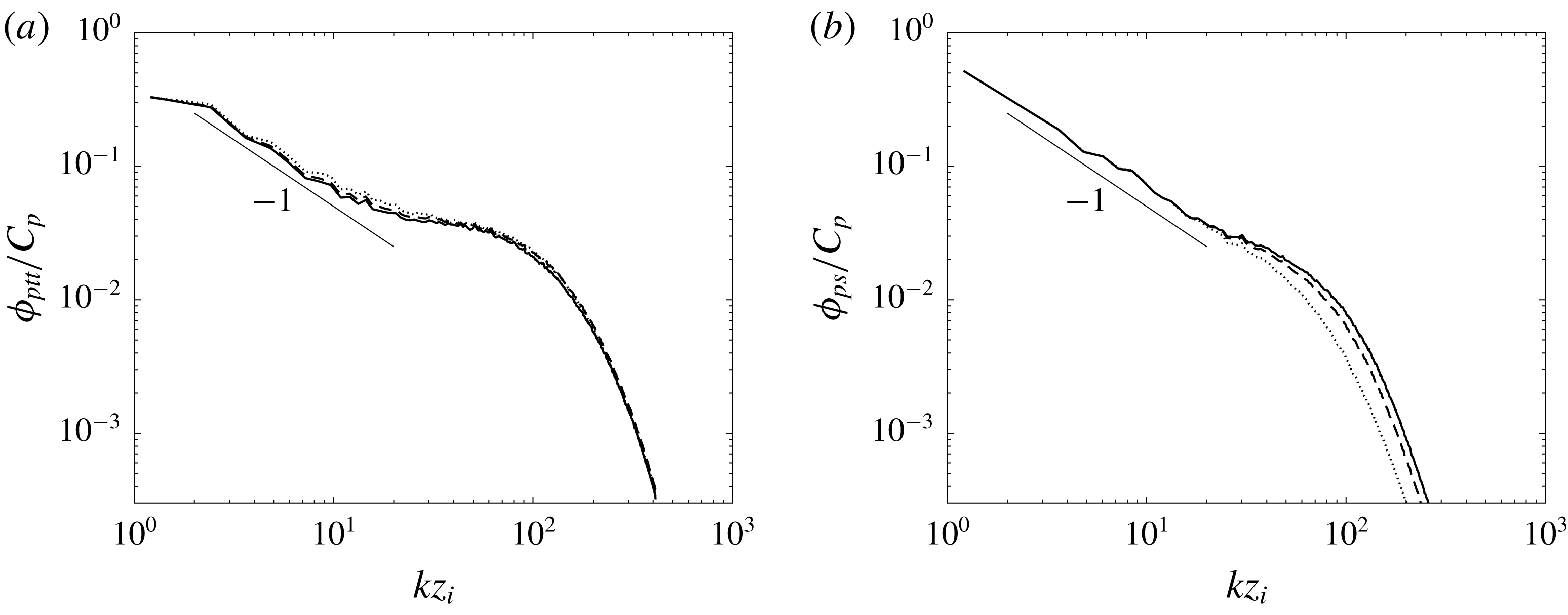
Figure 17. Pressure spectra of the (a) turbulent–turbulent and (b) rapid term contributions in the nearly neutral surface layer from LES using the Smagorinsky model, normalized by
 $C_{p}=u_{\ast }^{4}z_{i}$
. The lines represent heights of 16 m (solid), 20 m (dashed) and 30 m (dotted).
$C_{p}=u_{\ast }^{4}z_{i}$
. The lines represent heights of 16 m (solid), 20 m (dashed) and 30 m (dotted).
The pressure–strain-rate cospectra (figure 16), on the other hand, are dominated by the buoyancy contribution. Therefore, the local-free-convection parameters are the correct scales for predicting the cospectra. These results indicate that the turbulent–turbulent pressure fluctuations, while large in magnitude, are not well correlated with the strain rate. The effects of these pressure fluctuations on the velocity field will be further investigated in a future study. The behaviours of the turbulent–turbulent contribution to the cospectra are more complex. It causes return to isotropy at scales near
 $kz\sim 0.1$
, but reverses sign at and causes anisotropy at larger scales, up to those near
$kz\sim 0.1$
, but reverses sign at and causes anisotropy at larger scales, up to those near
 $z_{i}$
, again suggesting that Rotta’s model may be inappropriate for such a convective surface layer.
$z_{i}$
, again suggesting that Rotta’s model may be inappropriate for such a convective surface layer.
The scaling exponent of
 $-5/3$
of the pressure spectrum (dominated by the turbulent–turbulent contribution) suggests that the pressure fluctuations are primarily caused by the (
$-5/3$
of the pressure spectrum (dominated by the turbulent–turbulent contribution) suggests that the pressure fluctuations are primarily caused by the (
 $z_{i}$
scale) large convective eddies sweeping the smaller convective eddies of scale
$z_{i}$
scale) large convective eddies sweeping the smaller convective eddies of scale
 $1/k$
, resulting in the same scaling exponent as the velocity spectrum. The pressure spectrum therefore can be predicted as
$1/k$
, resulting in the same scaling exponent as the velocity spectrum. The pressure spectrum therefore can be predicted as
 $$\begin{eqnarray}\unicode[STIX]{x1D719}_{p}(k)\propto w_{\ast }^{2}u_{f}^{2}(k)k^{-1}=w_{\ast }^{2}(\unicode[STIX]{x1D6FD}Qk^{-1})^{2/3}k^{-1}=w_{\ast }^{2}(\unicode[STIX]{x1D6FD}Q)^{2/3}k^{-5/3}.\end{eqnarray}$$
For
 $k=1/z_{i}$
,
$k=1/z_{i}$
,
 $\unicode[STIX]{x1D719}_{p}k$
is of the order of
$\unicode[STIX]{x1D719}_{p}k$
is of the order of
 $w_{\ast }^{4}$
. Therefore, the predicted pressure spectrum is also consistent with the scaling of the pressure variance.
$w_{\ast }^{4}$
. Therefore, the predicted pressure spectrum is also consistent with the scaling of the pressure variance.

Figure 18. Profiles of different contributions in the nearly neutral surface layer from LES: the (a) turbulent–turbulent and (b) rapid terms using the Smagorinsky model; the (c) turbulent–turbulent and (d) rapid terms using the Kosović model. The lines represent
 ${\mathcal{R}}_{11}$
(solid),
${\mathcal{R}}_{11}$
(solid),
 ${\mathcal{R}}_{22}$
(dotted),
${\mathcal{R}}_{22}$
(dotted),
 ${\mathcal{R}}_{33}$
(dashed) and
${\mathcal{R}}_{33}$
(dashed) and
 ${\mathcal{R}}_{13}$
(dash-dot).
${\mathcal{R}}_{13}$
(dash-dot).

Figure 19. Profiles of the mean velocity gradient in the nearly neutral surface layer from LES using the Smagorinsky model (solid), Kosović model (dashed) and Smagorinsky model (
 $512^{3}$
) (dotted).
$512^{3}$
) (dotted).
For the near neutral surface layer, the turbulent–turbulent and rapid contributions to the pressure spectrum are of similar magnitudes (figure 17), consistent with the results in figure 18, which show that,
 ${\mathcal{R}}_{\unicode[STIX]{x1D6FC}\unicode[STIX]{x1D6FC}}^{(t)}$
and
${\mathcal{R}}_{\unicode[STIX]{x1D6FC}\unicode[STIX]{x1D6FC}}^{(t)}$
and
 ${\mathcal{R}}_{\unicode[STIX]{x1D6FC}\unicode[STIX]{x1D6FC}}^{(r)}$
are of similar magnitudes and are both important to
${\mathcal{R}}_{\unicode[STIX]{x1D6FC}\unicode[STIX]{x1D6FC}}^{(r)}$
are of similar magnitudes and are both important to
 ${\mathcal{R}}_{\unicode[STIX]{x1D6FC}\unicode[STIX]{x1D6FC}}$
. The non-dimensional profiles are nearly constant in the surface layer, consistent with the neutral surface-layer scaling. Here
${\mathcal{R}}_{\unicode[STIX]{x1D6FC}\unicode[STIX]{x1D6FC}}$
. The non-dimensional profiles are nearly constant in the surface layer, consistent with the neutral surface-layer scaling. Here
 ${\mathcal{R}}_{\unicode[STIX]{x1D6FC}\unicode[STIX]{x1D6FC}}^{(t)}$
have the same signs as
${\mathcal{R}}_{\unicode[STIX]{x1D6FC}\unicode[STIX]{x1D6FC}}^{(t)}$
have the same signs as
 ${\mathcal{R}}_{\unicode[STIX]{x1D6FC}\unicode[STIX]{x1D6FC}}$
, causing energy redistribution from the
${\mathcal{R}}_{\unicode[STIX]{x1D6FC}\unicode[STIX]{x1D6FC}}$
, causing energy redistribution from the
 $u$
to
$u$
to
 $v$
and
$v$
and
 $w$
components, consistent with return to isotropy. However, the energy redistribution to
$w$
components, consistent with return to isotropy. However, the energy redistribution to
 $v$
is small. The rapid contributions
$v$
is small. The rapid contributions
 ${\mathcal{R}}_{11}^{(r)}$
and
${\mathcal{R}}_{11}^{(r)}$
and
 ${\mathcal{R}}_{22}^{(r)}$
are negative and positive respectively. However,
${\mathcal{R}}_{22}^{(r)}$
are negative and positive respectively. However,
 ${\mathcal{R}}_{33}^{(r)}$
is negative, impeding return to isotropy, although its magnitude is small. Thus
${\mathcal{R}}_{33}^{(r)}$
is negative, impeding return to isotropy, although its magnitude is small. Thus
 ${\mathcal{R}}_{\unicode[STIX]{x1D6FC}\unicode[STIX]{x1D6FC}}^{(t)}$
and
${\mathcal{R}}_{\unicode[STIX]{x1D6FC}\unicode[STIX]{x1D6FC}}^{(t)}$
and
 ${\mathcal{R}}_{\unicode[STIX]{x1D6FC}\unicode[STIX]{x1D6FC}}^{(r)}$
are primarily responsible for redistributing energy from the streamwise to the vertical components and from the streamwise to the spanwise components respectively. Within the first few grid points, the non-dimensional mean shear typically shows an overshoot for the Smagorinsky model (figure 19). However,
${\mathcal{R}}_{\unicode[STIX]{x1D6FC}\unicode[STIX]{x1D6FC}}^{(r)}$
are primarily responsible for redistributing energy from the streamwise to the vertical components and from the streamwise to the spanwise components respectively. Within the first few grid points, the non-dimensional mean shear typically shows an overshoot for the Smagorinsky model (figure 19). However,
 ${\mathcal{R}}_{\unicode[STIX]{x1D6FC}\unicode[STIX]{x1D6FC}}^{(r)}$
(figure 18
b) shows no sign of such a behaviour, most likely because the fluctuating strain rate is somewhat under-resolved there. The mean shear for the Kosović model (figure 19) has no overshoot, and
${\mathcal{R}}_{\unicode[STIX]{x1D6FC}\unicode[STIX]{x1D6FC}}^{(r)}$
(figure 18
b) shows no sign of such a behaviour, most likely because the fluctuating strain rate is somewhat under-resolved there. The mean shear for the Kosović model (figure 19) has no overshoot, and
 ${\mathcal{R}}_{\unicode[STIX]{x1D6FC}\unicode[STIX]{x1D6FC}}^{(r)}$
is resolved to a somewhat lesser extent than the Smagorinsky model.
${\mathcal{R}}_{\unicode[STIX]{x1D6FC}\unicode[STIX]{x1D6FC}}^{(r)}$
is resolved to a somewhat lesser extent than the Smagorinsky model.

Figure 20. Pressure–strain-rate cospectra of the source term contributions in the nearly neutral surface layer at 16 m from LES using (a) the Smagorinsky model and (b) the Kosović model. The lines represent the total (solid), rapid (dash-dot) and turbulent–turbulent (dotted) contributions. Here
 $C_{\unicode[STIX]{x1D6FC}\unicode[STIX]{x1D6FC}}=C_{\unicode[STIX]{x1D6FC}\unicode[STIX]{x1D6FC}}^{\prime }/u_{\ast }^{3}$
. For clarity, some of the cospectra have been shifted vertically.
$C_{\unicode[STIX]{x1D6FC}\unicode[STIX]{x1D6FC}}=C_{\unicode[STIX]{x1D6FC}\unicode[STIX]{x1D6FC}}^{\prime }/u_{\ast }^{3}$
. For clarity, some of the cospectra have been shifted vertically.

Figure 21. Pressure–strain-rate cospectra of the source term contributions in the moderately convective surface layer at 16 m from LES using (a) the Smagorinsky model and (b) the Kosović model. The lines represent the total (solid), buoyancy (dashed) and turbulent–turbulent (dotted) contributions. Here
 $C_{\unicode[STIX]{x1D6FC}\unicode[STIX]{x1D6FC}}=C_{\unicode[STIX]{x1D6FC}\unicode[STIX]{x1D6FC}}^{\prime }/u_{\ast }^{3}$
. For clarity, some of the cospectra have been shifted vertically.
$C_{\unicode[STIX]{x1D6FC}\unicode[STIX]{x1D6FC}}=C_{\unicode[STIX]{x1D6FC}\unicode[STIX]{x1D6FC}}^{\prime }/u_{\ast }^{3}$
. For clarity, some of the cospectra have been shifted vertically.
The pressure–strain-rate cospectra for the near neutral surface layer at 16 m and the contributions from the source terms are shown in figure 20. For
 $kz\approx 1$
, the turbulent–turbulent contributions to
$kz\approx 1$
, the turbulent–turbulent contributions to
 $C_{11}$
,
$C_{11}$
,
 $C_{22}$
and
$C_{22}$
and
 $C_{33}$
have the same signs as
$C_{33}$
have the same signs as
 ${\mathcal{R}}_{11}^{(t)}$
,
${\mathcal{R}}_{11}^{(t)}$
,
 ${\mathcal{R}}_{22}^{(t)}$
and
${\mathcal{R}}_{22}^{(t)}$
and
 ${\mathcal{R}}_{33}^{(t)}$
shown in figure 18(a) (the contribution to
${\mathcal{R}}_{33}^{(t)}$
shown in figure 18(a) (the contribution to
 $C_{22}$
changes sign for
$C_{22}$
changes sign for
 $kz\gg 1$
). The rapid pressure contribution to
$kz\gg 1$
). The rapid pressure contribution to
 $C_{11}$
also has the same sign as
$C_{11}$
also has the same sign as
 ${\mathcal{R}}_{11}^{(r)}$
,
${\mathcal{R}}_{11}^{(r)}$
,
 ${\mathcal{R}}_{22}^{(r)}$
and
${\mathcal{R}}_{22}^{(r)}$
and
 ${\mathcal{R}}_{33}^{(r)}$
shown in figure 18(b), Thus while
${\mathcal{R}}_{33}^{(r)}$
shown in figure 18(b), Thus while
 $w$
receives energy through the turbulent–turbulent contribution at these scales, the
$w$
receives energy through the turbulent–turbulent contribution at these scales, the
 $v$
component does so primarily through the rapid contribution. Both the turbulent–turbulent and rapid contributions to
$v$
component does so primarily through the rapid contribution. Both the turbulent–turbulent and rapid contributions to
 $C_{13}$
are positive, causing return to isotropy.
$C_{13}$
are positive, causing return to isotropy.
For larger scales (
 $kz<0.3$
), the turbulent–turbulent contributions to
$kz<0.3$
), the turbulent–turbulent contributions to
 $C_{11}$
and
$C_{11}$
and
 $C_{33}$
reverse signs, and are positive and negative respectively, while the contribution to
$C_{33}$
reverse signs, and are positive and negative respectively, while the contribution to
 $C_{22}$
still has the same sign as for
$C_{22}$
still has the same sign as for
 $kz\approx 1$
. Thus, energy is redistributed from
$kz\approx 1$
. Thus, energy is redistributed from
 $w$
to
$w$
to
 $u$
and
$u$
and
 $v$
, thereby causing anisotropy at these scales, which is similar to the buoyancy contribution in the convective surface layer. The rapid contribution to
$v$
, thereby causing anisotropy at these scales, which is similar to the buoyancy contribution in the convective surface layer. The rapid contribution to
 $C_{11}$
is still negative. Interestingly, the rapid contribution to
$C_{11}$
is still negative. Interestingly, the rapid contribution to
 $C_{33}$
is now positive. The contribution to
$C_{33}$
is now positive. The contribution to
 $C_{22}$
also reverses sign, although at a smaller wavenumber. Thus the rapid contributions cause energy redistribution from
$C_{22}$
also reverses sign, although at a smaller wavenumber. Thus the rapid contributions cause energy redistribution from
 $u$
and
$u$
and
 $v$
to
$v$
to
 $w$
, opposite to the turbulent–turbulent contributions. The turbulent–turbulent contribution to
$w$
, opposite to the turbulent–turbulent contributions. The turbulent–turbulent contribution to
 $C_{13}$
also appears to reverse sign, resulting in anisotropy. The rapid contribution still positive, causing return to isotropy.
$C_{13}$
also appears to reverse sign, resulting in anisotropy. The rapid contribution still positive, causing return to isotropy.
For the moderately convective surface layer, the buoyancy contributions to the pressure–strain-rate cospectra (figure 21) have the same signs as those for the strongly convective surface layer. The turbulent–turbulent contributions near
 $kz=1$
have the same signs as
$kz=1$
have the same signs as
 ${\mathcal{R}}_{\unicode[STIX]{x1D6FC}\unicode[STIX]{x1D6FC}}$
. Similar to those for the strongly convective and near neutral surface layers, they also change signs as the scale increases. Thus, there are two redistribution processes for the turbulent–turbulent contribution, one at scales of order
${\mathcal{R}}_{\unicode[STIX]{x1D6FC}\unicode[STIX]{x1D6FC}}$
. Similar to those for the strongly convective and near neutral surface layers, they also change signs as the scale increases. Thus, there are two redistribution processes for the turbulent–turbulent contribution, one at scales of order
 $z$
and one at larger scales. Figures 16, 20 and 21 indicate that the relative magnitudes of the contributions at these scales and therefore the total turbulent–turbulent contributions vary with the stability condition (
$z$
and one at larger scales. Figures 16, 20 and 21 indicate that the relative magnitudes of the contributions at these scales and therefore the total turbulent–turbulent contributions vary with the stability condition (
 $z_{i}/L$
and
$z_{i}/L$
and
 $z/L$
). Thus Rotta’s model is likely to be inappropriate as a general model for all stability conditions.
$z/L$
). Thus Rotta’s model is likely to be inappropriate as a general model for all stability conditions.

Figure 22. Profiles of the (a) free-space and (b) wall reflection contributions to the pressure variance from the different source terms in the strongly convective surface layer from LES using the Smagorinsky model: buoyancy (dashed) and turbulent–turbulent (dotted). The total is represented by a solid line.

Figure 23. Profiles of the (a) free-space and (b) wall reflection contributions to the pressure variance from the different source terms in the nearly neutral surface layer from LES using the Smagorinsky model: rapid (dash-dot) and turbulent–turbulent (dotted). The total is represented by a solid line.
3.5 Effects of wall reflection
In this subsection we examine the effects of the wall on the pressure–strain-rate correlation. As mentioned in the Introduction, the pressure is decomposed into the free-space pressure,
 $p_{f}$
, the wall reflection,
$p_{f}$
, the wall reflection,
 $p_{w}$
, ((2.3) and (2.6) respectively) and the harmonic pressure,
$p_{w}$
, ((2.3) and (2.6) respectively) and the harmonic pressure,
 $p_{h}$
. We first examine the variances of
$p_{h}$
. We first examine the variances of
 $p_{f}$
and
$p_{f}$
and
 $p_{w}$
as well as the contributions from the different sources. For the strongly convective surface layer, the free-space pressure variance,
$p_{w}$
as well as the contributions from the different sources. For the strongly convective surface layer, the free-space pressure variance,
 $\unicode[STIX]{x1D70E}_{p_{f}}^{2}$
, increases with
$\unicode[STIX]{x1D70E}_{p_{f}}^{2}$
, increases with
 $z$
, primarily due to the turbulent–turbulent source (figure 22). The wall reflection
$z$
, primarily due to the turbulent–turbulent source (figure 22). The wall reflection
 $\unicode[STIX]{x1D70E}_{p_{w}}^{2}$
decreases nearly exponentially with increasing
$\unicode[STIX]{x1D70E}_{p_{w}}^{2}$
decreases nearly exponentially with increasing
 $z$
, with the
$z$
, with the
 $1/e$
point at approximately
$1/e$
point at approximately
 $z/z_{i}=0.1$
. The
$z/z_{i}=0.1$
. The
 $1/e$
points for the buoyancy and turbulent–turbulent contributions are approximately at
$1/e$
points for the buoyancy and turbulent–turbulent contributions are approximately at
 $z/z_{i}=0.13$
and 0.04 respectively. Since the depth of influence of the wall reflection depends on the coherence length of the (reflected) pressure source terms, these results suggest that the dominant length scale of the source terms is of the order of
$z/z_{i}=0.13$
and 0.04 respectively. Since the depth of influence of the wall reflection depends on the coherence length of the (reflected) pressure source terms, these results suggest that the dominant length scale of the source terms is of the order of
 $0.1z_{i}$
, and that the turbulent–turbulent source has a much smaller coherence length. For the near neutral surface layer,
$0.1z_{i}$
, and that the turbulent–turbulent source has a much smaller coherence length. For the near neutral surface layer,
 $\unicode[STIX]{x1D70E}_{p_{f}}^{2}$
decreases somewhat with increasing
$\unicode[STIX]{x1D70E}_{p_{f}}^{2}$
decreases somewhat with increasing
 $z$
, with the turbulent–turbulent source having the larger contribution (figure 23). The wall reflection
$z$
, with the turbulent–turbulent source having the larger contribution (figure 23). The wall reflection
 $\unicode[STIX]{x1D70E}_{p_{w}}^{2}$
decreases to the
$\unicode[STIX]{x1D70E}_{p_{w}}^{2}$
decreases to the
 $1/e$
point at approximately
$1/e$
point at approximately
 $z/z_{i}=0.04$
, faster than in the strongly convective surface layer. The rapid and turbulent–turbulent contributions to
$z/z_{i}=0.04$
, faster than in the strongly convective surface layer. The rapid and turbulent–turbulent contributions to
 $\unicode[STIX]{x1D70E}_{p_{w}}^{2}$
have approximately the same magnitude, in contrast to their contributions to
$\unicode[STIX]{x1D70E}_{p_{w}}^{2}$
have approximately the same magnitude, in contrast to their contributions to
 $\unicode[STIX]{x1D70E}_{p_{f}}^{2}$
, indicating that the rapid source has a larger coherence length.
$\unicode[STIX]{x1D70E}_{p_{f}}^{2}$
, indicating that the rapid source has a larger coherence length.
Figure 24 shows the free-space contribution,
 ${\mathcal{R}}_{f\unicode[STIX]{x1D6FC}\unicode[STIX]{x1D6FC}}$
, the wall reflection,
${\mathcal{R}}_{f\unicode[STIX]{x1D6FC}\unicode[STIX]{x1D6FC}}$
, the wall reflection,
 ${\mathcal{R}}_{w\unicode[STIX]{x1D6FC}\unicode[STIX]{x1D6FC}}$
, and the harmonic contribution,
${\mathcal{R}}_{w\unicode[STIX]{x1D6FC}\unicode[STIX]{x1D6FC}}$
, and the harmonic contribution,
 ${\mathcal{R}}_{h\unicode[STIX]{x1D6FC}\unicode[STIX]{x1D6FC}}$
, to
${\mathcal{R}}_{h\unicode[STIX]{x1D6FC}\unicode[STIX]{x1D6FC}}$
, to
 ${\mathcal{R}}_{\unicode[STIX]{x1D6FC}\unicode[STIX]{x1D6FC}}$
for the strongly convective surface layer. Throughout the surface layer
${\mathcal{R}}_{\unicode[STIX]{x1D6FC}\unicode[STIX]{x1D6FC}}$
for the strongly convective surface layer. Throughout the surface layer
 ${\mathcal{R}}_{f\unicode[STIX]{x1D6FC}\unicode[STIX]{x1D6FC}}$
varies slowly, except very close to the wall, which is due to the logarithmic behaviour discussed in § 3.1. It has the same sign as
${\mathcal{R}}_{f\unicode[STIX]{x1D6FC}\unicode[STIX]{x1D6FC}}$
varies slowly, except very close to the wall, which is due to the logarithmic behaviour discussed in § 3.1. It has the same sign as
 ${\mathcal{R}}_{\unicode[STIX]{x1D6FC}\unicode[STIX]{x1D6FC}}$
, indicating that the root cause of the surface-layer anisotropy lies in the pressure source terms, not the wall reflection or the harmonic pressure. This behaviour is because the flow is driven in the vertical direction by buoyancy, thereby having the tendency to redistribute energy from the vertical velocity component to the horizontal components. By definition
${\mathcal{R}}_{\unicode[STIX]{x1D6FC}\unicode[STIX]{x1D6FC}}$
, indicating that the root cause of the surface-layer anisotropy lies in the pressure source terms, not the wall reflection or the harmonic pressure. This behaviour is because the flow is driven in the vertical direction by buoyancy, thereby having the tendency to redistribute energy from the vertical velocity component to the horizontal components. By definition
 ${\mathcal{R}}_{w\unicode[STIX]{x1D6FC}\unicode[STIX]{x1D6FC}}$
equals
${\mathcal{R}}_{w\unicode[STIX]{x1D6FC}\unicode[STIX]{x1D6FC}}$
equals
 ${\mathcal{R}}_{f\unicode[STIX]{x1D6FC}\unicode[STIX]{x1D6FC}}$
on the surface and decays with increasing
${\mathcal{R}}_{f\unicode[STIX]{x1D6FC}\unicode[STIX]{x1D6FC}}$
on the surface and decays with increasing
 $z$
, as expected. It is most significant for
$z$
, as expected. It is most significant for
 $z/z_{i}<0.1$
, indicating that the wall reflection enhances the anisotropy in this region. The
$z/z_{i}<0.1$
, indicating that the wall reflection enhances the anisotropy in this region. The
 $1/e$
point is at approximately
$1/e$
point is at approximately
 $z/z_{i}=0.02$
, smaller than the value (0.1) for the pressure variance, likely due to the decrease of the correlation between the reflected pressure and the strain rate with increasing
$z/z_{i}=0.02$
, smaller than the value (0.1) for the pressure variance, likely due to the decrease of the correlation between the reflected pressure and the strain rate with increasing
 $z$
. Figure 24 shows that
$z$
. Figure 24 shows that
 ${\mathcal{R}}_{h\unicode[STIX]{x1D6FC}\unicode[STIX]{x1D6FC}}$
is relatively small.
${\mathcal{R}}_{h\unicode[STIX]{x1D6FC}\unicode[STIX]{x1D6FC}}$
is relatively small.
To further understand the free-space and wall reflection contributions, we compute the buoyancy and turbulent–turbulent parts (figures 25 and 26 respectively). For
 $z/z_{i}<0.1$
,
$z/z_{i}<0.1$
,
 ${\mathcal{R}}_{f\unicode[STIX]{x1D6FC}\unicode[STIX]{x1D6FC}}$
is dominated by the buoyancy part,
${\mathcal{R}}_{f\unicode[STIX]{x1D6FC}\unicode[STIX]{x1D6FC}}$
is dominated by the buoyancy part,
 ${\mathcal{R}}_{f\unicode[STIX]{x1D6FC}\unicode[STIX]{x1D6FC}}^{(b)}$
, whereas above
${\mathcal{R}}_{f\unicode[STIX]{x1D6FC}\unicode[STIX]{x1D6FC}}^{(b)}$
, whereas above
 $z/z_{i}=0.1$
the turbulent–turbulent part,
$z/z_{i}=0.1$
the turbulent–turbulent part,
 ${\mathcal{R}}_{f\unicode[STIX]{x1D6FC}\unicode[STIX]{x1D6FC}}^{(t)}$
, dominates. It is interesting that for
${\mathcal{R}}_{f\unicode[STIX]{x1D6FC}\unicode[STIX]{x1D6FC}}^{(t)}$
, dominates. It is interesting that for
 $z/z_{i}<0.04$
,
$z/z_{i}<0.04$
,
 ${\mathcal{R}}_{f\unicode[STIX]{x1D6FC}\unicode[STIX]{x1D6FC}}^{(t)}$
has the opposite signs to
${\mathcal{R}}_{f\unicode[STIX]{x1D6FC}\unicode[STIX]{x1D6FC}}^{(t)}$
has the opposite signs to
 ${\mathcal{R}}_{f\unicode[STIX]{x1D6FC}\unicode[STIX]{x1D6FC}}$
. However,
${\mathcal{R}}_{f\unicode[STIX]{x1D6FC}\unicode[STIX]{x1D6FC}}$
. However,
 ${\mathcal{R}}_{w\unicode[STIX]{x1D6FC}\unicode[STIX]{x1D6FC}}$
is dominated by
${\mathcal{R}}_{w\unicode[STIX]{x1D6FC}\unicode[STIX]{x1D6FC}}$
is dominated by
 ${\mathcal{R}}_{w\unicode[STIX]{x1D6FC}\unicode[STIX]{x1D6FC}}^{(b)}$
. The
${\mathcal{R}}_{w\unicode[STIX]{x1D6FC}\unicode[STIX]{x1D6FC}}^{(b)}$
. The
 $1/e$
point is approximately at
$1/e$
point is approximately at
 $z/z_{i}=0.04$
, larger than
$z/z_{i}=0.04$
, larger than
 ${\mathcal{R}}_{w\unicode[STIX]{x1D6FC}\unicode[STIX]{x1D6FC}}$
, due to the larger coherence of the reflected buoyancy source. The results suggest that the length scales of the motions contributing to
${\mathcal{R}}_{w\unicode[STIX]{x1D6FC}\unicode[STIX]{x1D6FC}}$
, due to the larger coherence of the reflected buoyancy source. The results suggest that the length scales of the motions contributing to
 ${\mathcal{R}}_{w\unicode[STIX]{x1D6FC}\unicode[STIX]{x1D6FC}}^{(t)}$
are small, resulting in smaller wall reflection.
${\mathcal{R}}_{w\unicode[STIX]{x1D6FC}\unicode[STIX]{x1D6FC}}^{(t)}$
are small, resulting in smaller wall reflection.

Figure 24. Profiles of the (a) free-space, (b) wall reflection and (c) harmonic contributions to
 ${\mathcal{R}}_{\unicode[STIX]{x1D6FC}\unicode[STIX]{x1D6FC}}$
in the strongly convective surface layer from LES using the Smagorinsky model. The lines represent
${\mathcal{R}}_{\unicode[STIX]{x1D6FC}\unicode[STIX]{x1D6FC}}$
in the strongly convective surface layer from LES using the Smagorinsky model. The lines represent
 ${\mathcal{R}}_{11}$
(solid),
${\mathcal{R}}_{11}$
(solid),
 ${\mathcal{R}}_{22}$
(dotted) and
${\mathcal{R}}_{22}$
(dotted) and
 ${\mathcal{R}}_{33}$
(dashed).
${\mathcal{R}}_{33}$
(dashed).

Figure 25. Profiles of the (a) free-space and (b) wall reflection contributions to
 ${\mathcal{R}}_{\unicode[STIX]{x1D6FC}\unicode[STIX]{x1D6FC}}$
from the turbulent–turbulent source term in the strongly convective surface layer from LES using the Smagorinsky model. The lines represent
${\mathcal{R}}_{\unicode[STIX]{x1D6FC}\unicode[STIX]{x1D6FC}}$
from the turbulent–turbulent source term in the strongly convective surface layer from LES using the Smagorinsky model. The lines represent
 ${\mathcal{R}}_{11}$
(solid),
${\mathcal{R}}_{11}$
(solid),
 ${\mathcal{R}}_{22}$
(dotted) and
${\mathcal{R}}_{22}$
(dotted) and
 ${\mathcal{R}}_{33}$
(dashed).
${\mathcal{R}}_{33}$
(dashed).

Figure 26. Profiles of the (a) free-space and (b) wall reflection contributions to
 ${\mathcal{R}}_{\unicode[STIX]{x1D6FC}\unicode[STIX]{x1D6FC}}$
from the buoyancy source term in the strongly convective surface layer from LES using the Smagorinsky model. The lines represent
${\mathcal{R}}_{\unicode[STIX]{x1D6FC}\unicode[STIX]{x1D6FC}}$
from the buoyancy source term in the strongly convective surface layer from LES using the Smagorinsky model. The lines represent
 ${\mathcal{R}}_{11}$
(solid),
${\mathcal{R}}_{11}$
(solid),
 ${\mathcal{R}}_{22}$
(dotted) and
${\mathcal{R}}_{22}$
(dotted) and
 ${\mathcal{R}}_{33}$
(dashed).
${\mathcal{R}}_{33}$
(dashed).

Figure 27. Profiles of the (a) free-space and (b) wall reflection contributions to
 ${\mathcal{R}}_{\unicode[STIX]{x1D6FC}\unicode[STIX]{x1D6FC}}$
in the nearly neutral surface layer from LES using the Smagorinsky model. The lines represent
${\mathcal{R}}_{\unicode[STIX]{x1D6FC}\unicode[STIX]{x1D6FC}}$
in the nearly neutral surface layer from LES using the Smagorinsky model. The lines represent
 ${\mathcal{R}}_{11}$
(solid),
${\mathcal{R}}_{11}$
(solid),
 ${\mathcal{R}}_{22}$
(dotted) and
${\mathcal{R}}_{22}$
(dotted) and
 ${\mathcal{R}}_{33}$
(dashed).
${\mathcal{R}}_{33}$
(dashed).
For the near neutral surface layer (figure 27),
 ${\mathcal{R}}_{f\unicode[STIX]{x1D6FC}\unicode[STIX]{x1D6FC}}$
varies slowly except for
${\mathcal{R}}_{f\unicode[STIX]{x1D6FC}\unicode[STIX]{x1D6FC}}$
varies slowly except for
 $z/z_{i}<0.02$
where it decreases with
$z/z_{i}<0.02$
where it decreases with
 $z$
, due to the under-resolution of the strain rate by the LES near the surface. For most of the surface layer
$z$
, due to the under-resolution of the strain rate by the LES near the surface. For most of the surface layer
 ${\mathcal{R}}_{w\unicode[STIX]{x1D6FC}\unicode[STIX]{x1D6FC}}$
is much smaller than the free-space contribution, due to the under-resolution of the strain rate very close to the wall and the fast decreases of the reflected pressure and its correlation with the strain rate (note that the wall reflection contribution does not increase for
${\mathcal{R}}_{w\unicode[STIX]{x1D6FC}\unicode[STIX]{x1D6FC}}$
is much smaller than the free-space contribution, due to the under-resolution of the strain rate very close to the wall and the fast decreases of the reflected pressure and its correlation with the strain rate (note that the wall reflection contribution does not increase for
 $z/z_{i}>0.02$
where the strain rate are better resolved, as figure 27
a shows). The wall reflection contribution to
$z/z_{i}>0.02$
where the strain rate are better resolved, as figure 27
a shows). The wall reflection contribution to
 ${\mathcal{R}}_{13}$
is also small (not shown).
${\mathcal{R}}_{13}$
is also small (not shown).
The results in this subsection can help us understand the effects of the wall on the pressure–strain-rate correlation in convective and neutral surface layers. In a neutral surface layer, the redistribution occurs due to the shear production injecting energy into the streamwise component, rendering it the largest. The wall is not essential for the energy redistribution that causes return to isotropy, i.e. it can occur without a wall, as in the case of a homogeneous shear flow. The presence of the wall has two opposing effects: wall reflection of the pressure source enhances the process, while wall blocking of the vertical velocity impedes it.
In a convective surface layer, buoyancy and pressure transport drive the flow in the vertical direction. Therefore the flow naturally redistributes energy from the vertical component to the horizontal components. This is consistent with the results that the free-space pressure contribution to the pressure–strain-rate correlation (from the source term in the Poisson equation) has the opposite sign to that in a neutral surface layer. In the meantime, wall blocking restricts the vertical velocity fluctuations, making the vertical component the smallest of the three. The energy redistribution and the restriction of the vertical fluctuations together result in surface-layer anisotropy. Therefore, the wall is not necessary for the redistribution but is essential to the anisotropy. On the other hand, wall reflection of the pressure source, while enhancing the energy redistribution (similar to the neutral surface layer), is not the root cause of the anisotropy. From the modelling point of view, if a model for the source term contribution does not have the correct sign (one that leads to anisotropy), modelling the wall reflection will not give the pressure–strain-rate correlation the correct behaviour. Therefore, accurate modelling of the contribution from the source term is essential for modelling the pressure–strain-rate correlation and the generation of anisotropy.
4 Discussion and conclusions
In the present work we studied the pressure fluctuations and the pressure–strain-rate correlation in convective and near neutral atmospheric surface layers. Their scaling properties, the spectral characteristics, the contributions from the different pressure sources and the wall reflection were investigated using high-resolution (from 512
 $^{3}$
to 2048
$^{3}$
to 2048
 $^{3}$
) LES and through spectral predictions. The understanding gained helped address three important issues: it elucidates the physical mechanism for generating the anisotropy in convective surface layers, provides strong support to MMO and clarifies the issue of modelling the turbulent–turbulent contribution as a return-to-isotropy term (Rotta’s model).
$^{3}$
) LES and through spectral predictions. The understanding gained helped address three important issues: it elucidates the physical mechanism for generating the anisotropy in convective surface layers, provides strong support to MMO and clarifies the issue of modelling the turbulent–turbulent contribution as a return-to-isotropy term (Rotta’s model).
A number of steps were taken to ensure that the results, especially the scaling properties, are not affected by the SGS model and the LES resolutions near the surface. Two SGS models, the Smagorinsky model and the Kosović model were employed and the results obtained were consistent. The pressure variance, the pressure–strain-rate correlation and the pressure–strain-rate cospectra in the convective surface layer are found to be sensitive to the LES resolution, consistent with the observation of Miles et al. (Reference Miles, Wyngaard and Otte2004). The pressure–strain-rate correlation in the neutral surface layer is approximately 80 % resolved at the tenth grid point from the surface. The overshoot of the non-dimensional mean shear within the first few grid points for the Smagorinsky model does not result in an over-prediction of the rapid contribution of the pressure–strain-rate correlation, due to the under-resolution of the strain rate there.
For the strongly convective surface layer, the pressure–strain-rate correlation was found to have the mixed-layer scaling (
 $w_{\ast }^{3}/z_{i}$
), with
$w_{\ast }^{3}/z_{i}$
), with
 ${\mathcal{R}}_{11}$
,
${\mathcal{R}}_{11}$
,
 ${\mathcal{R}}_{22}$
and
${\mathcal{R}}_{22}$
and
 ${\mathcal{R}}_{13}$
being positive and
${\mathcal{R}}_{13}$
being positive and
 ${\mathcal{R}}_{33}$
being negative, consistent with the results of Nguyen et al. (Reference Nguyen, Horst, Oncley and Tong2013) and Nguyen & Tong (Reference Nguyen and Tong2015), indicating that the normal components cause anisotropy in the velocity variances. Near the surface, they vary logarithmically, which can be predicted by extending Townsend’s attached-eddy model to the pressure–strain-rate correlation or using the pressure–strain-rate cospectra predicted (3.5). For the neutral surface layer, the pressure–strain-rate scales with
${\mathcal{R}}_{33}$
being negative, consistent with the results of Nguyen et al. (Reference Nguyen, Horst, Oncley and Tong2013) and Nguyen & Tong (Reference Nguyen and Tong2015), indicating that the normal components cause anisotropy in the velocity variances. Near the surface, they vary logarithmically, which can be predicted by extending Townsend’s attached-eddy model to the pressure–strain-rate correlation or using the pressure–strain-rate cospectra predicted (3.5). For the neutral surface layer, the pressure–strain-rate scales with
 $u_{\ast }^{3}/z$
, with
$u_{\ast }^{3}/z$
, with
 ${\mathcal{R}}_{11}$
being negative and
${\mathcal{R}}_{11}$
being negative and
 ${\mathcal{R}}_{22}$
,
${\mathcal{R}}_{22}$
,
 ${\mathcal{R}}_{33}$
and
${\mathcal{R}}_{33}$
and
 ${\mathcal{R}}_{13}$
being positive, consistent with its usual role of causing return to isotropy. In the convective–dynamic layer of a moderately convective surface layer (
${\mathcal{R}}_{13}$
being positive, consistent with its usual role of causing return to isotropy. In the convective–dynamic layer of a moderately convective surface layer (
 $-z/L\sim 1$
), it has both mixed-layer and surface-layer contributions, but has apparent surface-layer scaling, inconsistent with the mixed-layer scaling of the horizontal velocity variances. This inconsistency is an inherent problem for single-point statistics in this multi-scale phenomenon. As pointed out by Tong & Nguyen (Reference Tong and Nguyen2015), general surface-layer similarity therefore needs to be considered for multi-point statistics in the framework of MMO similarity instead of the original Monin–Obukhov similarity.
$-z/L\sim 1$
), it has both mixed-layer and surface-layer contributions, but has apparent surface-layer scaling, inconsistent with the mixed-layer scaling of the horizontal velocity variances. This inconsistency is an inherent problem for single-point statistics in this multi-scale phenomenon. As pointed out by Tong & Nguyen (Reference Tong and Nguyen2015), general surface-layer similarity therefore needs to be considered for multi-point statistics in the framework of MMO similarity instead of the original Monin–Obukhov similarity.
A decomposition of the pressure into different sources contributions shows that the behaviour of the pressure–strain-rate correlation in the strongly convective surface layer is primarily due to the buoyancy contribution. The turbulent–turbulent contribution, while significant, plays only a minor role. In the near neutral surface layer, both the turbulent–turbulent and rapid contributions are important, and are responsible for redistributing energy from the streamwise to the vertical components and from the streamwise to the cross-stream components, respectively.
The pressure variance has the mixed-layer scaling (
 $w_{\ast }^{4}$
) in both strongly and moderately convective surface layers, similar to the horizontal velocity variances. It is dominated by the turbulent–turbulent contribution. In the near neutral surface layer, it scales with
$w_{\ast }^{4}$
) in both strongly and moderately convective surface layers, similar to the horizontal velocity variances. It is dominated by the turbulent–turbulent contribution. In the near neutral surface layer, it scales with
 $u_{\ast }^{4}$
, with both the turbulent–turbulent and rapid contributions being important.
$u_{\ast }^{4}$
, with both the turbulent–turbulent and rapid contributions being important.
The pressure spectrum at the large scales (
 $kz<1$
) in the strongly convective surface layer has an approximate
$kz<1$
) in the strongly convective surface layer has an approximate
 $k^{-5/3}$
scaling range, different from the prediction of
$k^{-5/3}$
scaling range, different from the prediction of
 $k^{-7/3}$
scaling using the surface-layer parameters. It is dominated by the turbulent–turbulent contribution, which involves both the mixed-layer and local-free-convection scales: The large convective eddies sweep the smaller, local convective eddies, resulting an approximate
$k^{-7/3}$
scaling using the surface-layer parameters. It is dominated by the turbulent–turbulent contribution, which involves both the mixed-layer and local-free-convection scales: The large convective eddies sweep the smaller, local convective eddies, resulting an approximate
 $k^{-5/3}$
scaling range. Therefore it does not appear to follow the MMO similarity. The buoyancy contribution has a
$k^{-5/3}$
scaling range. Therefore it does not appear to follow the MMO similarity. The buoyancy contribution has a
 $k^{-7/3}$
scaling range, consistent with our prediction, and follows MMO. Thus the pressure spectrum is not completely determined by the surface-layer parameters.
$k^{-7/3}$
scaling range, consistent with our prediction, and follows MMO. Thus the pressure spectrum is not completely determined by the surface-layer parameters.
The pressure–strain-rate cospectra in the convective surface layer are dominated by the buoyancy contribution, not the turbulent–turbulent (inertial) contribution, in contrast to the pressure spectrum, and thus have the local-free-convection (surface-layer) scaling, consistent with our prediction of a
 $k^{-1}$
scaling range. The different scaling properties of the pressure spectrum and the pressure–strain-rate cospectra result from the their different dominant contributions. The former is dominated by the turbulent–turbulent contribution, which involves both mixed-layer and surface-layer scales, whereas the latter is dominated by the buoyancy contribution. The different scaling properties also indicate that only the buoyancy contribution of the pressure fluctuations are well correlated with the strain rate, whereas the turbulent–turbulent contribution is not, and consequently does not contribute significantly to the redistribution of energy. Therefore, buoyancy effects associated with the large convective eddies are largely responsible for causing the surface-layer anisotropy in the velocity variances as suggested by Nguyen et al. (Reference Nguyen, Horst, Oncley and Tong2013) and Nguyen & Tong (Reference Nguyen and Tong2015).
$k^{-1}$
scaling range. The different scaling properties of the pressure spectrum and the pressure–strain-rate cospectra result from the their different dominant contributions. The former is dominated by the turbulent–turbulent contribution, which involves both mixed-layer and surface-layer scales, whereas the latter is dominated by the buoyancy contribution. The different scaling properties also indicate that only the buoyancy contribution of the pressure fluctuations are well correlated with the strain rate, whereas the turbulent–turbulent contribution is not, and consequently does not contribute significantly to the redistribution of energy. Therefore, buoyancy effects associated with the large convective eddies are largely responsible for causing the surface-layer anisotropy in the velocity variances as suggested by Nguyen et al. (Reference Nguyen, Horst, Oncley and Tong2013) and Nguyen & Tong (Reference Nguyen and Tong2015).
A physical picture of the generation of the anisotropy in the normal components of the Reynolds stress tensor in convective surface layers emerges from our analysis. The buoyancy production injects energy into the vertical velocity, at scales that increases with the height from the surface (in the mixed layer most of the energy is at scales of order
 $z_{i}$
). The energy then flows towards the surface through the pressure transport. The pressure–strain-rate correlation, which is primarily due to the buoyancy (stacking) effects generated by the density (temperature) fluctuations in the convective eddies, subsequently redistributes the energy to the horizontal components, at scales ranging from
$z_{i}$
). The energy then flows towards the surface through the pressure transport. The pressure–strain-rate correlation, which is primarily due to the buoyancy (stacking) effects generated by the density (temperature) fluctuations in the convective eddies, subsequently redistributes the energy to the horizontal components, at scales ranging from
 $-L$
to
$-L$
to
 $z_{i}$
, resulting in anisotropy. The turbulent–turbulent (inertial) contribution, e.g. downward flow impinging on the surface, only plays a minor role, that is, the pressure responsible for most of the energy redistribution is not the dynamic pressure.
$z_{i}$
, resulting in anisotropy. The turbulent–turbulent (inertial) contribution, e.g. downward flow impinging on the surface, only plays a minor role, that is, the pressure responsible for most of the energy redistribution is not the dynamic pressure.
For the neutral surface layer, both the turbulent–turbulent and rapid contributions to the pressure spectrum have a
 $k^{-1}$
scaling range, consistent with our prediction using the surface-layer parameters. The pressure–strain-rate cospectra near
$k^{-1}$
scaling range, consistent with our prediction using the surface-layer parameters. The pressure–strain-rate cospectra near
 $kz=1$
dominate the contribution to
$kz=1$
dominate the contribution to
 ${\mathcal{R}}_{\unicode[STIX]{x1D6FC}\unicode[STIX]{x1D6FC}}$
, with a negative
${\mathcal{R}}_{\unicode[STIX]{x1D6FC}\unicode[STIX]{x1D6FC}}$
, with a negative
 $C_{11}$
and positive
$C_{11}$
and positive
 $C_{33}$
and
$C_{33}$
and
 $C_{22}$
, causing energy redistribution from the
$C_{22}$
, causing energy redistribution from the
 $u$
component to the
$u$
component to the
 $v$
and
$v$
and
 $w$
components and return to isotropy. These behaviours are primarily due to the turbulent–turbulent contribution. The rapid contribution causes redistribution of energy from
$w$
components and return to isotropy. These behaviours are primarily due to the turbulent–turbulent contribution. The rapid contribution causes redistribution of energy from
 $u$
and
$u$
and
 $w$
to
$w$
to
 $v$
, for which the physics responsible is unclear. The cospectrum
$v$
, for which the physics responsible is unclear. The cospectrum
 $C_{13}$
near
$C_{13}$
near
 $kz=1$
is positive and also dominates
$kz=1$
is positive and also dominates
 ${\mathcal{R}}_{13}$
, with both the turbulent–turbulent and rapid contributions being important. For larger scales (
${\mathcal{R}}_{13}$
, with both the turbulent–turbulent and rapid contributions being important. For larger scales (
 $kz<1$
), however,
$kz<1$
), however,
 $C_{33}$
becomes negative while
$C_{33}$
becomes negative while
 $C_{11}$
is nearly zero. This behaviour is primarily due to the turbulent–turbulent contribution, which redistributes energy from
$C_{11}$
is nearly zero. This behaviour is primarily due to the turbulent–turbulent contribution, which redistributes energy from
 $w$
to
$w$
to
 $u$
and
$u$
and
 $v$
. These results indicate that the large eddies in the neutral surface layer redistribute energy among the velocity components in a way somewhat similar to the convective eddies, thus having the tendency to cause anisotropy. The rapid contribution redistributes energy from
$v$
. These results indicate that the large eddies in the neutral surface layer redistribute energy among the velocity components in a way somewhat similar to the convective eddies, thus having the tendency to cause anisotropy. The rapid contribution redistributes energy from
 $u$
and
$u$
and
 $v$
to
$v$
to
 $w$
, opposite to the turbulent–turbulent contribution. The turbulent–turbulent contribution to
$w$
, opposite to the turbulent–turbulent contribution. The turbulent–turbulent contribution to
 ${\mathcal{R}}_{13}$
also reverses sign, causing anisotropy.
${\mathcal{R}}_{13}$
also reverses sign, causing anisotropy.
In the convective–dynamic layer of a moderately convective surface layer (
 $-z/L<1$
), the mean shear is strong near the surface. For
$-z/L<1$
), the mean shear is strong near the surface. For
 $-kL\ll 1$
the pressure strain-rate cospectra are similar to those in a strongly convective surface layer, with
$-kL\ll 1$
the pressure strain-rate cospectra are similar to those in a strongly convective surface layer, with
 $C_{11}$
being positive and
$C_{11}$
being positive and
 $C_{33}$
being negative. For
$C_{33}$
being negative. For
 $-kL\gg 1$
(but
$-kL\gg 1$
(but
 $kz<1$
) they have a similar scaling range as those in a neutral surface layer, with
$kz<1$
) they have a similar scaling range as those in a neutral surface layer, with
 $C_{11}$
being negative and
$C_{11}$
being negative and
 $C_{33}$
being positive, causing return to isotropy, similar to a neutral surface layer. Thus, there are two redistribution processes occurring at two distinct scale ranges, one near
$C_{33}$
being positive, causing return to isotropy, similar to a neutral surface layer. Thus, there are two redistribution processes occurring at two distinct scale ranges, one near
 $z$
and one beyond. They do not appear to interact directly, although the former can be modified by the latter when the mean shear is altered from the neutral limit.
$z$
and one beyond. They do not appear to interact directly, although the former can be modified by the latter when the mean shear is altered from the neutral limit.
The change of sign of the pressure–strain-rate cospectra near
 $-kL\sim 1$
indicates that
$-kL\sim 1$
indicates that
 $-L$
is imposed on the horizontal directions as a length scale by the pressure–strain-rate correlation. Therefore, turbulence spectra and other multipoint statistics depend on
$-L$
is imposed on the horizontal directions as a length scale by the pressure–strain-rate correlation. Therefore, turbulence spectra and other multipoint statistics depend on
 $kL$
and have different scaling ranges for
$kL$
and have different scaling ranges for
 $-kL>1$
and
$-kL>1$
and
 $-kL<1$
, providing strong support for MMO.
$-kL<1$
, providing strong support for MMO.
To examine the role of the source terms in the Poisson equation and the wall reflection, we decomposed the pressure into free-space, wall reflection and harmonic pressures and obtained their contributions to the pressure–strain-rate correlation. The free-space contribution has the same sign as the total, indicating that the source terms are the root cause of the behaviours of the pressure–strain-rate correlation, and thus the anisotropy of the velocity covariances in the convective surface layer. The wall reflection is significant for
 $z/z_{i}<0.1$
in the convective surface layer, thus enhancing anisotropy there. This result also indicates that the coherence length of the source is of the order of
$z/z_{i}<0.1$
in the convective surface layer, thus enhancing anisotropy there. This result also indicates that the coherence length of the source is of the order of
 $0.1z_{i}$
, the approximate height of the surface layer. The wall reflection contribution comes primarily from the buoyancy source, due to its large-scale nature. In the near neutral surface layer the wall reflection contribution is small, mainly due to the smaller coherence length of the pressure source, although the under-resolution of the strain rate near the surface by LES may play a minor role.
$0.1z_{i}$
, the approximate height of the surface layer. The wall reflection contribution comes primarily from the buoyancy source, due to its large-scale nature. In the near neutral surface layer the wall reflection contribution is small, mainly due to the smaller coherence length of the pressure source, although the under-resolution of the strain rate near the surface by LES may play a minor role.
The present study can help clarify the common practice of modelling the turbulent–turbulent contribution to the pressure–strain-rate correlation as a return-to-isotropy term. In a decaying turbulent velocity field without external influences energy is redistributed from the larger to the smaller component at a rate determined by the anisotropy and the integral time scale. Rotta’s model is therefore appropriate. In a turbulent flow with anisotropic forcing (production), the situation is more complex. In a neutral boundary layer it causes return to isotropy, since the streamwise component, which is forced, is the largest component. In a convective surface layer there are two forcing mechanisms (shear and buoyancy production). Their contributions therefore depend on the stability condition. In weakly and moderately surface layers it causes return to isotropy, similar to the neutral surface layer. In strongly convective surface layers, it has small magnitudes, although the signs are consistent with return to isotropy. Rotta’s model, on the other hand, predicts a large energy redistribution (return to isotropy) due to the large difference between the vertical and horizontal velocity variances, inconsistent with our results. As a result, Rotta’s model is appropriate for decaying turbulence and neutral boundary layers (in the log layer), but not for the convective surface layer.
The results in the present study, especially the pressure–strain-rate cospectra, also have potential implications on understanding the dynamics of the surface-layer structure. For example, the sign changes of the pressure–strain-rate cospectra at
 $kz\ll 1$
may have implications on the large-scale dynamics, e.g. the long streaks that have received much attention in the literature. The dynamics of such a structure are expected to be strongly influenced by the interaction between the pressure and the strain rate at large scales.
$kz\ll 1$
may have implications on the large-scale dynamics, e.g. the long streaks that have received much attention in the literature. The dynamics of such a structure are expected to be strongly influenced by the interaction between the pressure and the strain rate at large scales.
Acknowledgements
We would like to acknowledge high-performance computing support from Yellowstone (ark:/85065/d7wd3xhc) provided by NCAR’s Computational and Information Systems Laboratory. This work was supported by the US National Science Foundation through grants nos AGS-1335995 and AGS-1561190.