


1 Introduction
The interaction of surface waves with a vertically sheared current plays an important role in the ocean (see a review by Peregrine (Reference Peregrine1976)). For example, Banner & Phillips (Reference Banner and Phillips1974), Banner & Song (Reference Banner and Song2002) and Yao & Wu (Reference Yao and Wu2005) demonstrated that the presence of a shear current varying with depth affects the breaking limit of surface waves. See also the experimental studies of current–wave interactions by Thomas (Reference Thomas1981, Reference Thomas1990) and Swan, Cummins & James (Reference Swan, Cummins and James2001).
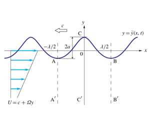
The present work considers stability of the two-dimensional periodic motion of steady deep-water waves of symmetric profile on a linear shear current with the horizontal velocity distribution  $U(y)=c+\unicode[STIX]{x1D6FA}y$ in the frame of reference moving to the left with the wave speed
  $c$, where the shear strength
  $\unicode[STIX]{x1D6FA}$ is a constant, as shown in figure 1(a). Note that waves for
  $\unicode[STIX]{x1D6FA}>0$ and
  $\unicode[STIX]{x1D6FA}<0$ are referred to as upstream and downstream propagating waves, respectively.

Figure 1. Deep-water waves on a linear shear current and conformal mapping of the flow domain. The mapping functions among the  $\unicode[STIX]{x1D701}$-,
  $\unicode[STIX]{x1D6EC}$- and
  $\hat{\unicode[STIX]{x1D6EC}}$-planes are given by (2.16).
  $U$: the horizontal velocity of the shear current in the frame of reference moving to the left with the wave speed
  $c$,
$c$,  $\unicode[STIX]{x1D6FA}$: the shear strength,
  $\unicode[STIX]{x1D706}$: the wavelength and
  $a$: the wave amplitude (one half of the crest-to-trough height).
Since the vorticity in a two-dimensional incompressible and inviscid flow is conserved and the vorticity of a linear shear current is constant ( $=-\,\unicode[STIX]{x1D6FA}$), any perturbations must be irrotational. Therefore, we can formulate the present problem within the framework of potential flow theory and introduce the complex velocity potential for perturbed wave motions. It should be noted that, although the waves of interest are irrotational even for
  $\unicode[STIX]{x1D6FA}\neq 0$, in this paper, only the waves without a shear current are referred to as irrotational waves (
 $\unicode[STIX]{x1D6FA}=0$). On the basis of this formulation, the full Euler system has been numerically solved by Simmen & Saffman (Reference Simmen and Saffman1985), Teles da Silva & Peregrine (Reference Teles da Silva and Peregrine1988) and Vanden-Broeck (Reference Vanden-Broeck1996) for steady waves, and by Choi (Reference Choi2009) and Moreira & Chacaltana (Reference Moreira and Chacaltana2015) for unsteady waves. It has been known that the limiting form of steady waves of symmetric profile can have a corner at the wave crest with an inner angle of
  $120^{\circ }$ which is independent of the shear strength
  $\unicode[STIX]{x1D6FA}$ (Milne-Thomson Reference Milne-Thomson1968, p. 403, §14.50), similarly to the case of irrotational waves (
 $\unicode[STIX]{x1D6FA}=0$).
Steady wave solutions for  $\unicode[STIX]{x1D6FA}\neq 0$ are determined by two dimensionless parameters,
  $\unicode[STIX]{x1D6FA}_{\ast }=\unicode[STIX]{x1D6FA}/\sqrt{gk}$ and the wave steepness
  $a_{\ast }=ak$, where
  $g$,
$g$,  $k$ and
  $a$ denote the gravitational acceleration, the wavenumber and the wave amplitude (one half of the crest-to-trough height), respectively. In this work, we numerically investigate the linear stability of non-overhanging periodic waves for
  $-3\leqslant \unicode[STIX]{x1D6FA}_{\ast }\leqslant 0.6$ and a wide range of the wave steepnesses
  $a_{\ast }$, for which instabilities due to super- and sub-harmonic disturbances are observed. For upstream propagating waves (
 $\unicode[STIX]{x1D6FA}>0$), while overhanging wave profiles appear for large values of
  $\unicode[STIX]{x1D6FA}_{\ast }$ (Simmen & Saffman Reference Simmen and Saffman1985; Teles da Silva & Peregrine Reference Teles da Silva and Peregrine1988; Vanden-Broeck Reference Vanden-Broeck1996; Dyachenko & Hur Reference Dyachenko and Hur2019a,Reference Dyachenko and Hurb), a spectral method for computation of the steady solutions requires a number
  $N$ of Fourier modes of the order of
  $10^{4}$, which is much greater than that in our numerical stability analysis, typically,
  $N\leqslant 2^{9}(=512)$.
In the absence of a shear current, the linear stability of steady solutions of the full Euler system for finite-amplitude irrotational waves ( $\unicode[STIX]{x1D6FA}=0$) has been studied extensively by, for example, Longuet-Higgins (Reference Longuet-Higgins1978a,Reference Longuet-Higginsb), McLean (Reference McLean1982) and Tanaka (Reference Tanaka1983) for periodic gravity waves; Zhang & Melville (Reference Zhang and Melville1987) for gravity–capillary waves; Chen & Saffman (Reference Chen and Saffman1985) and Tiron & Choi (Reference Tiron and Choi2012) for capillary waves; Tanaka (Reference Tanaka1986) for solitary waves. In particular, Longuet-Higgins (Reference Longuet-Higgins1978b) and Tanaka (Reference Tanaka1983) found numerically two typical behaviours of eigenvalues of the linearized system for small disturbances to steady wave solutions, (i) a ‘bubble of instability’ due to subharmonic disturbances, as shown in figure 8(a1) and (ii) the ‘Tanaka instability’ due to superharmonic disturbances, as shown in figure 5(a), respectively (MacKay & Saffman Reference MacKay and Saffman1986). Here sub- and super-harmonic disturbances are those with horizontal scale longer and shorter than steady waves, respectively. In this work, the focus is on how these two instabilities change with the shear strength
  $\unicode[STIX]{x1D6FA}$.
In the presence of a linear shear current, weakly nonlinear theories for small-amplitude waves have been first developed. For steady waves, asymptotic theories were presented by Benjamin (Reference Benjamin1962) and Miroshnikov (Reference Miroshnikov2002) for weakly and strongly nonlinear solitary waves, respectively, Simmen & Saffman (Reference Simmen and Saffman1985) for deep-water waves and Hsu et al. (Reference Hsu, Francius, Montalvo and Kharif2016) for gravity–capillary waves on water of finite depth. For unsteady waves, Freeman & Johnson (Reference Freeman and Johnson1970) and Choi (Reference Choi2003) obtained the weakly nonlinear Korteweg–de Vries equation and a strongly nonlinear long wave model for shallow-water waves, respectively, while Thomas, Kharif & Manna (Reference Thomas, Kharif and Manna2012) derived a nonlinear Schrödinger (NLS) equation for the envelope of periodic waves on water of finite and infinite depth. Using the NLS equation, Thomas et al. (Reference Thomas, Kharif and Manna2012) and Francius & Kharif (Reference Francius and Kharif2017) investigated the effect of a shear current on the Benjamin–Feir instability, which occurs at relatively small amplitudes, and pointed out that the deep-water limit of coupling between the mean flow and the background vorticity is essential for the evaluation of the stability of deep-water waves.
A few attempts have been made previously for numerical investigation of the linear stability of finite-amplitude waves on a linear shear current ( $\unicode[STIX]{x1D6FA}\neq 0$), including Okamura & Oikawa (Reference Okamura and Oikawa1989) and Francius & Kharif (Reference Francius and Kharif2017), who used the full Euler system for periodic waves on water of finite depth. Okamura & Oikawa (Reference Okamura and Oikawa1989) examined the three-dimensional instability of two-dimensional steady waves, similarly to McLean (Reference McLean1982) for irrotational waves (
 $\unicode[STIX]{x1D6FA}=0$). Francius & Kharif (Reference Francius and Kharif2017) investigated two-dimensional instability for a wide range of the shear strengths,
  $\unicode[STIX]{x1D6FA}$, and compared the results with their weakly nonlinear theory (Thomas et al. Reference Thomas, Kharif and Manna2012). In particular, Francius & Kharif (Reference Francius and Kharif2017) discovered re-stabilization of the Benjamin–Feir instability with a change of
  $\unicode[STIX]{x1D6FA}$ for upstream propagating waves (
 $\unicode[STIX]{x1D6FA}>0$), which may be dominated by new bands of instability. Notice that the propagation direction of waves in this work is opposite to that in Francius & Kharif (Reference Francius and Kharif2017) and so is the sign of
  $\unicode[STIX]{x1D6FA}$ for upstream and downstream propagating waves.
Saffman (Reference Saffman1985) analytically proved, using Zakharov’s Hamiltonian formulation for  $\unicode[STIX]{x1D6FA}=0$ (Zakharov Reference Zakharov1968), that, at the critical point of the Tanaka superharmonic instability, exchange of stability occurs and the wave energy is an extremum as a function of wave amplitude, as numerically shown by Tanaka (Reference Tanaka1983, Reference Tanaka1985). Wahlén (Reference Wahlén2007) derived a canonical Hamiltonian system for water waves on a linear shear current by generalizing Zakharov’s formulation with a suitable choice of canonical variables. Sato & Yamada (Reference Sato and Yamada2019) pointed out that translational symmetry in a canonical Hamiltonian system is essential in the Tanaka instability, and analytically predicted from the result by Wahlén (Reference Wahlén2007) that the same type of instability can occur even in the presence of a linear shear current.
In Francius & Kharif (Reference Francius and Kharif2017), the maximum wave steepness is  $ka=0.2$ for
  $-0.6\leqslant \unicode[STIX]{x1D6FA}/\sqrt{gk}\leqslant 1$, which is much less than
  $ka\simeq 0.4292$, at which the Tanaka superharmonic instability for
  $\unicode[STIX]{x1D6FA}=0$ occurs. Thus, their stability results are limited to moderate wave steepness, mainly due to slow convergence of their numerical methods. Furthermore, no stability analysis has been presented for superharmonic disturbances in previous studies. In this work, we apply one of the conformal mapping techniques to the linear stability analysis of large-amplitude waves in § 4, and present some numerical examples of both sub- and super-harmonic instabilities in § 5.
To compute large-amplitude steady waves, the hodograph transformation has been widely used. Its original idea is to interchange the dependent and independent variables such that spatial coordinates are functions of the velocity potential  $\unicode[STIX]{x1D719}$ and the streamfunction
  $\unicode[STIX]{x1D713}$. Its major advantage is that the water surface is located on the real axis, or
  $\unicode[STIX]{x1D713}=0$ in the complex function
  $f(=\unicode[STIX]{x1D719}+\text{i}\unicode[STIX]{x1D713})$-plane where the flow domain is conformally mapped. On the other hand, for unsteady waves, the streamfunction
  $\unicode[STIX]{x1D713}$ is not constant and vary with time on the free surface (Longuet-Higgins Reference Longuet-Higgins1978a,Reference Longuet-Higginsb). Therefore, to study the stability of large-amplitude waves, we should generalize the idea of the hodograph transformation to unsteady waves. Such a generalization has been explored for unsteady waves to find a transformation, where the unknown location of the free surface is mapped on the real axis
  $\unicode[STIX]{x1D702}=0$ of a complex plane, or the
  $\unicode[STIX]{x1D701}(=\unicode[STIX]{x1D709}+\text{i}\unicode[STIX]{x1D702})$-plane, which is guaranteed by the Riemann mapping theory. It has been shown that the time-dependent transformation can be found by solving the nonlinear evolution equations and this idea has been applied to various water wave problems by Ovshannikov (Reference Ovshannikov1974), Dyachenko, Zakharov & Kuznetsov (Reference Dyachenko, Zakharov and Kuznetsov1996), Choi & Camassa (Reference Choi and Camassa1999), Chalikov & Sheinin (Reference Chalikov and Sheinin2005) and Murashige & Choi (Reference Murashige and Choi2017) for
  $\unicode[STIX]{x1D6FA}=0$, and by Ruban (Reference Ruban2008), Choi (Reference Choi2009) and Dyachenko & Hur (Reference Dyachenko and Hur2019a,Reference Dyachenko and Hurb) for
  $\unicode[STIX]{x1D6FA}\neq 0$. The same formulation has been also used for stability analysis by Tiron & Choi (Reference Tiron and Choi2012) for pure capillary waves and Dosaev, Troitskaya & Shishina (Reference Dosaev, Troitskaya and Shishina2017) for the Benjamin–Feir instability of deep-water gravity waves on a linear shear current. In this work, we apply the idea of this time-dependent transformation to study the linear stability of large-amplitude waves.
The paper is organized as follows. Formulation of the problem using conformal mapping is presented in § 2. Computed results for steady waves of symmetric profile are shown in § 3. The method of linear stability analysis following the Floquet theory in the conformally mapped planes is shown in § 4. Numerical examples of linear stability analysis for super- and sub-harmonic disturbances are summarized and discussed in § 5. Section 6 concludes this work.
2 Formulation of the problem
2.1 Formulation in the physical plane
Consider the stability of the periodic steady motion of deep-water gravity waves progressing to the left in permanent form with constant speed  $c$ on a linear shear current, as shown in figure 1(a). The profile of the periodic steady waves is assumed to be symmetric with respect to the vertical line passing through the wave crest. It is also assumed that the fluid motion is two-dimensional in the vertical cross-section
  $(x,y)$ along the propagation direction of the waves, and that the fluid is inviscid and incompressible. The origin is placed such that the wave profile
  $y={\tilde{y}}(x,t)$ satisfies the zero mean level condition
 $$\begin{eqnarray}\displaystyle \int _{0}^{\unicode[STIX]{x1D706}}{\tilde{y}}(x,t)\,\text{d}x=0,\end{eqnarray}$$
 where  $\unicode[STIX]{x1D706}$ is the wavelength and
  $t$ denotes the time.
It is convenient to formulate the problem in the frame of reference moving with the waves so that the horizontal velocity of a linear shear current is given by  $U=c+\unicode[STIX]{x1D6FA}y$ with constant
  $\unicode[STIX]{x1D6FA}$. Then, the fluid velocity vector
  $\boldsymbol{U}$ can be written as
 $$\begin{eqnarray}\boldsymbol{U}=\left(\begin{array}{@{}c@{}}U\\ V\end{array}\right)=\left(\begin{array}{@{}c@{}}\unicode[STIX]{x1D6FA}y\\ 0\end{array}\right)+\left(\begin{array}{@{}c@{}}u\\ v\end{array}\right),\end{eqnarray}$$
with the bottom boundary condition
 $$\begin{eqnarray}\left(\begin{array}{@{}c@{}}u\\ v\end{array}\right)\rightarrow \left(\begin{array}{@{}c@{}}c\\ 0\end{array}\right)\quad \text{as }y\rightarrow -\infty .\end{eqnarray}$$
 In the case of no wave motion,  $u=c$ and
  $v=0$. From conservation of vorticity for two-dimensional flows, as the vorticity remains constant (
 $=-\,\unicode[STIX]{x1D6FA}$) if it is initially constant, the perturbed wave motion given by
  $(u,v)$ must be irrotational. Thus we can introduce the complex velocity potential
  $f$ defined by
 $$\begin{eqnarray}f(z,t)=\unicode[STIX]{x1D719}(x,y,t)+\text{i}\unicode[STIX]{x1D713}(x,y,t)\quad \text{with}\quad \displaystyle \frac{\unicode[STIX]{x2202}f}{\unicode[STIX]{x2202}z}=w=u-\text{i}v,\end{eqnarray}$$
 where  $z=x+\text{i}y$ and
  $w=u-\text{i}v$ denote the complex coordinate and the complex velocity, respectively. In addition, from the mass conservation law given by
  $U_{x}+V_{y}=0$, there exists a streamfunction
  $\unicode[STIX]{x1D6F9}$ defined by
 $$\begin{eqnarray}U=\unicode[STIX]{x1D6F9}_{y}\quad \text{and}\quad V=-\unicode[STIX]{x1D6F9}_{x}.\end{eqnarray}$$
 From (2.2) and (2.4),  $\unicode[STIX]{x1D6F9}$ is related to
  $\unicode[STIX]{x1D713}=\text{Im}\{f\}$ by
 $$\begin{eqnarray}\unicode[STIX]{x1D6F9}=\displaystyle {\textstyle \frac{1}{2}}\unicode[STIX]{x1D6FA}y^{2}+\unicode[STIX]{x1D713}.\end{eqnarray}$$
 When physical variables are non-dimensionalized, with respect to  $c$ and
  $k(=2\unicode[STIX]{x03C0}/\unicode[STIX]{x1D706})$, as
 $$\begin{eqnarray}z_{\ast }=kz,\quad t_{\ast }=ckt,\quad f_{\ast }=\displaystyle \frac{f}{(c/k)},\quad {\tilde{y}}_{\ast }=k{\tilde{y}},\end{eqnarray}$$
the following dimensionless parameters appear in the problem:
 $$\begin{eqnarray}a_{\ast }=ka,\quad \unicode[STIX]{x1D6FA}_{\ast }=\displaystyle \frac{\unicode[STIX]{x1D6FA}}{\sqrt{gk}},\quad c_{\ast }=\displaystyle \frac{c}{\sqrt{g/k}},\end{eqnarray}$$
 where  $a$ denotes the wave amplitude (one half of the crest-to-trough height) and
  $a_{\ast }=ka$ is the wave steepness. Henceforth the asterisks for dimensionless variables will be omitted for brevity.
The boundary conditions at the water surface  $y={\tilde{y}}(x,t)$ are given, from the kinematic condition, by
 $$\begin{eqnarray}{\tilde{y}}_{t}+\left(\unicode[STIX]{x1D719}_{x}+\displaystyle \frac{\unicode[STIX]{x1D6FA}}{c}{\tilde{y}}\right){\tilde{y}}_{x}=\unicode[STIX]{x1D719}_{y}\quad \text{at }y={\tilde{y}}(x,t),\end{eqnarray}$$
and, from the dynamic condition, by
 $$\begin{eqnarray}\unicode[STIX]{x1D719}_{t}+\displaystyle \frac{1}{c^{2}}{\tilde{y}}+\displaystyle \frac{1}{2}({\unicode[STIX]{x1D719}_{x}}^{2}+{\unicode[STIX]{x1D719}_{y}}^{2})+\displaystyle \frac{\unicode[STIX]{x1D6FA}}{c}({\tilde{y}}\unicode[STIX]{x1D719}_{x}-\unicode[STIX]{x1D713})=B(t)\quad \text{at }y={\tilde{y}}(x,t),\end{eqnarray}$$
 where an arbitrary function  $B(t)$ can be absorbed into
  $\unicode[STIX]{x1D719}$. Also the bottom boundary condition (2.3) as
  $y\rightarrow -\infty$ can be rewritten as
 $$\begin{eqnarray}\displaystyle \frac{\unicode[STIX]{x2202}f}{\unicode[STIX]{x2202}z}=\unicode[STIX]{x1D719}_{x}+\text{i}\unicode[STIX]{x1D713}_{x}~\rightarrow ~1\quad \text{as }y\rightarrow -\infty .\end{eqnarray}$$
2.2 Unsteady conformal mapping of the flow domain
For linear stability analysis of large-amplitude steady waves, we introduce a conformal mapping technique (Dyachenko et al. Reference Dyachenko, Zakharov and Kuznetsov1996; Ruban Reference Ruban2008; Choi Reference Choi2009; Tiron & Choi Reference Tiron and Choi2012; Dosaev et al. Reference Dosaev, Troitskaya and Shishina2017; Murashige & Choi Reference Murashige and Choi2017; Dyachenko & Hur Reference Dyachenko and Hur2019a,Reference Dyachenko and Hurb) which maps the flow domain onto the lower half  $\unicode[STIX]{x1D702}<0$ of the
  $\unicode[STIX]{x1D701}$-plane (
 $\unicode[STIX]{x1D701}=\unicode[STIX]{x1D709}+\text{i}\unicode[STIX]{x1D702}$) or the unit disk
  $|\hat{\unicode[STIX]{x1D6EC}}|<1$ in the
  $\hat{\unicode[STIX]{x1D6EC}}$-plane (
 $\hat{\unicode[STIX]{x1D6EC}}=\hat{r}\text{e}^{\text{i}\hat{\unicode[STIX]{x1D717}}}$), as shown in figure 1. The time-varying water surface is always mapped onto the real axis
  $\unicode[STIX]{x1D702}=0$ in the
  $\unicode[STIX]{x1D701}$-plane or the unit circle
  $\hat{\unicode[STIX]{x1D6EC}}=\text{e}^{\text{i}\hat{\unicode[STIX]{x1D717}}}$ in the
  $\hat{\unicode[STIX]{x1D6EC}}$-plane.
Numerical computation of large-amplitude waves close to the limiting waves with a corner at the wave crest requires high resolution in space near the crest, and some auxiliary conformal mappings for it has been proposed (Tanaka Reference Tanaka1983; Murashige & Tanaka Reference Murashige and Tanaka2015; Lushnikov, Dyachenko & Silantyev Reference Lushnikov, Dyachenko and Silantyev2017). For irrotational waves ( $\unicode[STIX]{x1D6FA}=0$), Tanaka (Reference Tanaka1983) controlled the spatial resolution near the wave crest by conformally mapping the flow domain onto the unit disk in the
  $\hat{\unicode[STIX]{x1D6EC}}$-plane and succeeded in numerically capturing the Tanaka superharmonic instability occurring at a large amplitude (
 $ka\simeq 0.4292$). We apply this idea to the present problem for numerical investigation of the linear stability of large-amplitude waves subject to superharmonic disturbances.
2.2.1 The  $\unicode[STIX]{x1D701}$-plane for unsteady wave motion

In the  $\unicode[STIX]{x1D701}$-plane (
 $\unicode[STIX]{x1D701}=\unicode[STIX]{x1D709}+\text{i}\unicode[STIX]{x1D702}$), we choose
  $z=z(\unicode[STIX]{x1D701},t)$ and
  $f=f(\unicode[STIX]{x1D701},t)$ as dependent variables. Then, the mapping function between the
  $z$- and
  $\unicode[STIX]{x1D701}$-planes is given by a solution
  $z=z(\unicode[STIX]{x1D701},t)$ of the problem. The flow domain is conformally mapped onto the lower half
  $\unicode[STIX]{x1D702}<0$, as shown in figure 1(b), and the free surface boundary conditions, namely the kinematic and dynamic conditions, at the water surface
  $\unicode[STIX]{x1D702}=0$ are given, respectively, by
 $$\begin{eqnarray}x_{\unicode[STIX]{x1D709}}y_{t}-y_{\unicode[STIX]{x1D709}}x_{t}=-\left(\unicode[STIX]{x1D713}_{\unicode[STIX]{x1D709}}+\displaystyle \frac{\unicode[STIX]{x1D6FA}}{c}yy_{\unicode[STIX]{x1D709}}\right)\quad \text{at }\unicode[STIX]{x1D702}=0,\end{eqnarray}$$
and
 $$\begin{eqnarray}\unicode[STIX]{x1D719}_{t}-\displaystyle \frac{\unicode[STIX]{x1D719}_{\unicode[STIX]{x1D709}}}{J}(x_{\unicode[STIX]{x1D709}}x_{t}+y_{\unicode[STIX]{x1D709}}y_{t})+\displaystyle \frac{1}{c^{2}}y+\displaystyle \frac{1}{2J}({\unicode[STIX]{x1D719}_{\unicode[STIX]{x1D709}}}^{2}-{\unicode[STIX]{x1D713}_{\unicode[STIX]{x1D709}}}^{2})+\displaystyle \frac{\unicode[STIX]{x1D6FA}}{c}\left(\displaystyle \frac{\unicode[STIX]{x1D719}_{\unicode[STIX]{x1D709}}}{J}yx_{\unicode[STIX]{x1D709}}-\unicode[STIX]{x1D713}\right)=B(t)\quad \text{at }\unicode[STIX]{x1D702}=0,\end{eqnarray}$$
 where  $J$ is defined by
 $$\begin{eqnarray}J=\displaystyle \frac{\unicode[STIX]{x2202}(x,y)}{\unicode[STIX]{x2202}(\unicode[STIX]{x1D709},\unicode[STIX]{x1D702})}={x_{\unicode[STIX]{x1D709}}}^{2}+{y_{\unicode[STIX]{x1D709}}}^{2}.\end{eqnarray}$$
The bottom boundary condition (2.11) is satisfied with
 $$\begin{eqnarray}z\rightarrow \unicode[STIX]{x1D701}\quad \text{and}\quad f\rightarrow \unicode[STIX]{x1D701}\quad \text{as }\unicode[STIX]{x1D702}\rightarrow -\infty .\end{eqnarray}$$
Notice that Tiron & Choi (Reference Tiron and Choi2012) adopted alternative forms of the free surface boundary conditions given by (A 2) and (A 3) including the Hilbert transform, instead of (2.12) and (2.13), for linear stability analysis of capillary waves (see appendix A). In this work, we use (2.12) and (2.13) which do not require direct evaluation of the Hilbert transform, but the stability results from the two different forms would be identical.
2.2.2 The $\hat{\unicode[STIX]{x1D6EC}}$-plane for $2\unicode[STIX]{x03C0}$-periodic wave motion


For  $2\unicode[STIX]{x03C0}$-periodic wave motions, it is convenient to further map the flow domain onto the unit disk in the
  $\hat{\unicode[STIX]{x1D6EC}}$-plane, as shown in figure 1(d), where the spatial resolution at the water surface can be controlled for accurate computation of large-amplitude waves (Tanaka Reference Tanaka1983; Longuet-Higgins & Tanaka Reference Longuet-Higgins and Tanaka1997). The
  $\hat{\unicode[STIX]{x1D6EC}}$-plane is obtained by the following two transformations through the
  $\unicode[STIX]{x1D6EC}$-plane shown in figure 1(c):
 $$\begin{eqnarray}\unicode[STIX]{x1D6EC}=\text{e}^{-\text{i}\unicode[STIX]{x1D701}}\quad \text{and}\quad \unicode[STIX]{x1D6EC}=\displaystyle \frac{\hat{\unicode[STIX]{x1D6EC}}+\unicode[STIX]{x1D707}}{1+\unicode[STIX]{x1D707}\hat{\unicode[STIX]{x1D6EC}}}\quad (0\leqslant \unicode[STIX]{x1D707}<1).\end{eqnarray}$$
 Branch cuts are set to  $-\infty <\unicode[STIX]{x1D6EC}\leqslant 0$ and
  $-1/\unicode[STIX]{x1D707}\leqslant \hat{\unicode[STIX]{x1D6EC}}\leqslant -\unicode[STIX]{x1D707}$ along the real axes in the
  $\unicode[STIX]{x1D6EC}$- and
  $\hat{\unicode[STIX]{x1D6EC}}$-planes, respectively, such that
  $\log \unicode[STIX]{x1D6EC}$ is uniquely defined. The water surface is mapped onto the unit circle
  $\unicode[STIX]{x1D6EC}=\text{e}^{\text{i}\unicode[STIX]{x1D717}}$ or
  $\hat{\unicode[STIX]{x1D6EC}}=\text{e}^{\text{i}\hat{\unicode[STIX]{x1D717}}}$, and the argument
  $\unicode[STIX]{x1D717}$ in the
  $\unicode[STIX]{x1D6EC}$-plane is related to
  $\unicode[STIX]{x1D709}$ and the argument
  $\hat{\unicode[STIX]{x1D717}}$ in the
  $\hat{\unicode[STIX]{x1D6EC}}$-plane at the water surface, respectively, as
 $$\begin{eqnarray}\unicode[STIX]{x1D717}=-\unicode[STIX]{x1D709}\quad \text{and}\quad \tan \unicode[STIX]{x1D717}=\displaystyle \frac{(1-\unicode[STIX]{x1D707}^{2})\sin \hat{\unicode[STIX]{x1D717}}}{2\unicode[STIX]{x1D707}+(1+\unicode[STIX]{x1D707}^{2})\cos \hat{\unicode[STIX]{x1D717}}}\quad (-\unicode[STIX]{x03C0}\leqslant \unicode[STIX]{x1D709},\unicode[STIX]{x1D717},\hat{\unicode[STIX]{x1D717}}\leqslant \unicode[STIX]{x03C0}).\end{eqnarray}$$
 The wave crest  $\unicode[STIX]{x1D709}=0$ and trough
  $\unicode[STIX]{x1D709}=\pm \unicode[STIX]{x03C0}$ of
  $2\unicode[STIX]{x03C0}$-periodic steady waves are mapped onto
  $\unicode[STIX]{x1D717}=\hat{\unicode[STIX]{x1D717}}=0$ and
  $\unicode[STIX]{x1D717}=\hat{\unicode[STIX]{x1D717}}=\mp \unicode[STIX]{x03C0}$, respectively. When the water surface
  $\hat{\unicode[STIX]{x1D6EC}}=\text{e}^{\text{i}\hat{\unicode[STIX]{x1D717}}}$ is divided into a finite number of equal intervals in the
  $\hat{\unicode[STIX]{x1D6EC}}$-plane, the spatial resolution near the wave crest in the physical plane (the
  $z$-plane) increases with the parameter
  $\unicode[STIX]{x1D707}\in [0,1)$ in the mapping function (2.16). Also, the bottom
  $y\rightarrow -\infty$ is mapped onto
  $\unicode[STIX]{x1D6EC}=0$ or
  $\hat{\unicode[STIX]{x1D6EC}}=-\unicode[STIX]{x1D707}$.
Similarly to the  $\unicode[STIX]{x1D701}$-plane, we adopt
  $z$ and
  $f$ as dependent variables in the
  $\hat{\unicode[STIX]{x1D6EC}}$-plane. We write these dependent variables
  $z$ and
  $f$ in the
  $\hat{\unicode[STIX]{x1D6EC}}$-plane as
  $z=z(\hat{\unicode[STIX]{x1D6EC}},t)$ and
  $f=f(\hat{\unicode[STIX]{x1D6EC}},t)$, respectively, instead of
  $z=z(\unicode[STIX]{x1D701}(\hat{\unicode[STIX]{x1D6EC}}),t)$ and
  $f=f(\unicode[STIX]{x1D701}(\hat{\unicode[STIX]{x1D6EC}}),t)$, for convenience. The free surface boundary conditions, namely the kinematic and dynamic conditions, at the water surface
  $\hat{\unicode[STIX]{x1D6EC}}=\text{e}^{\text{i}\hat{\unicode[STIX]{x1D717}}}$ are given, respectively, by
 $$\begin{eqnarray}x_{\hat{\unicode[STIX]{x1D717}}}y_{t}-y_{\hat{\unicode[STIX]{x1D717}}}x_{t}=-\left(\unicode[STIX]{x1D713}_{\hat{\unicode[STIX]{x1D717}}}+\displaystyle \frac{\unicode[STIX]{x1D6FA}}{c}yy_{\hat{\unicode[STIX]{x1D717}}}\right)\quad \text{at }\hat{\unicode[STIX]{x1D6EC}}=\text{e}^{\text{i}\hat{\unicode[STIX]{x1D717}}},\end{eqnarray}$$
and
 $$\begin{eqnarray}\unicode[STIX]{x1D719}_{t}-\displaystyle \frac{\unicode[STIX]{x1D719}_{\hat{\unicode[STIX]{x1D717}}}}{{\hat{J}}}(x_{\hat{\unicode[STIX]{x1D717}}}x_{t}+y_{\hat{\unicode[STIX]{x1D717}}}y_{t})+\displaystyle \frac{1}{c^{2}}y+\displaystyle \frac{1}{2{\hat{J}}}({\unicode[STIX]{x1D719}_{\hat{\unicode[STIX]{x1D717}}}}^{2}-{\unicode[STIX]{x1D713}_{\hat{\unicode[STIX]{x1D717}}}}^{2})+\displaystyle \frac{\unicode[STIX]{x1D6FA}}{c}\left(\displaystyle \frac{\unicode[STIX]{x1D719}_{\hat{\unicode[STIX]{x1D717}}}}{{\hat{J}}}yx_{\hat{\unicode[STIX]{x1D717}}}-\unicode[STIX]{x1D713}\right)=B(t)\quad \text{at }\hat{\unicode[STIX]{x1D6EC}}=\text{e}^{\text{i}\hat{\unicode[STIX]{x1D717}}},\end{eqnarray}$$
 where  $-\unicode[STIX]{x03C0}\leqslant \hat{\unicode[STIX]{x1D717}}\leqslant \unicode[STIX]{x03C0}$ and
  ${\hat{J}}$ is defined by
 $$\begin{eqnarray}{\hat{J}}={x_{\hat{\unicode[STIX]{x1D717}}}}^{2}+{y_{\hat{\unicode[STIX]{x1D717}}}}^{2}.\end{eqnarray}$$
The bottom boundary condition (2.15) becomes
 $$\begin{eqnarray}z(\hat{\unicode[STIX]{x1D6EC}})\rightarrow \text{i}\log \unicode[STIX]{x1D6EC}(\hat{\unicode[STIX]{x1D6EC}})\quad \text{and}\quad f(\hat{\unicode[STIX]{x1D6EC}})\rightarrow \text{i}\log \unicode[STIX]{x1D6EC}(\hat{\unicode[STIX]{x1D6EC}})\quad \text{as }\hat{\unicode[STIX]{x1D6EC}}\rightarrow -\unicode[STIX]{x1D707},\end{eqnarray}$$
 where  $\unicode[STIX]{x1D6EC}=\unicode[STIX]{x1D6EC}(\hat{\unicode[STIX]{x1D6EC}})$ is given by (2.16).
3 Steady waves of symmetric profile
We write steady solutions of  $2\unicode[STIX]{x03C0}$-periodic waves of symmetric profile as
  $z=z_{0}(\unicode[STIX]{x1D701})$ and
  $f=f_{0}(\unicode[STIX]{x1D701})$ in the
  $\unicode[STIX]{x1D701}$-plane while
  $z=z_{0}(\hat{\unicode[STIX]{x1D6EC}})$ and
  $f=f_{0}(\hat{\unicode[STIX]{x1D6EC}})$ in the
  $\hat{\unicode[STIX]{x1D6EC}}$-plane. In their computations for
  $\unicode[STIX]{x1D6FA}=0$, Tanaka (Reference Tanaka1983) and Longuet-Higgins & Tanaka (Reference Longuet-Higgins and Tanaka1997) adopted
  $\unicode[STIX]{x1D6FE}$, as one of parameters for steady waves, which is defined by
 $$\begin{eqnarray}\unicode[STIX]{x1D6FE}=1-q_{crest}/q_{trough},\end{eqnarray}$$
 where  $q_{crest}$ and
  $q_{trough}$ denote the fluid velocity at the wave crest and trough in the frame of reference moving with steady waves, respectively. For a wide range of
  $\unicode[STIX]{x1D6FA}$, this parameter
  $\unicode[STIX]{x1D6FE}\in [0,1]$ monotonically increases with the wave steepness
  $ka$. The maximum wave steepness
  $ka$ of the limiting wave changes with the shear strength
  $\unicode[STIX]{x1D6FA}$, while the corresponding
  $\unicode[STIX]{x1D6FE}=1$ is invariant with respect to
  $\unicode[STIX]{x1D6FA}$ considered in this work, as shown in figure 7. Then we use this parameter
  $\unicode[STIX]{x1D6FE}$, instead of the wave steepness
  $ka$ for the computations of steady waves for
  $\unicode[STIX]{x1D6FA}\neq 0$.
3.1 Boundary conditions
In the  $\unicode[STIX]{x1D701}$-plane, the kinematic condition (2.12) for steady waves is reduced to
 $$\begin{eqnarray}\unicode[STIX]{x1D713}_{0\unicode[STIX]{x1D709}}=-\displaystyle \frac{\unicode[STIX]{x1D6FA}}{c}y_{0}y_{0\unicode[STIX]{x1D709}}~\quad \text{or}\quad ~\unicode[STIX]{x1D713}_{0}=-\displaystyle \frac{\unicode[STIX]{x1D6FA}}{2c}{y_{0}}^{2}+\,\text{constant}\quad \text{at }\unicode[STIX]{x1D702}=0.\end{eqnarray}$$
Substituting this into the dynamic condition (2.13), we get
 $$\begin{eqnarray}\left(\unicode[STIX]{x1D719}_{0\unicode[STIX]{x1D709}}+\displaystyle \frac{\unicode[STIX]{x1D6FA}}{c}y_{0}x_{0\unicode[STIX]{x1D709}}\right)^{2}-J_{0}\left(B_{0}-\displaystyle \frac{2}{c^{2}}y_{0}\right)=0\quad \text{at }\unicode[STIX]{x1D702}=0,\end{eqnarray}$$
 where  $-\unicode[STIX]{x03C0}\leqslant \unicode[STIX]{x1D709}\leqslant \unicode[STIX]{x03C0}$,
  $B_{0}$ is a real constant and
 $$\begin{eqnarray}J_{0}={x_{0\unicode[STIX]{x1D709}}}^{2}+{y_{0\unicode[STIX]{x1D709}}}^{2}.\end{eqnarray}$$
 In the  $\hat{\unicode[STIX]{x1D6EC}}$-plane, (3.3) can be transformed using (2.17) to
 $$\begin{eqnarray}\unicode[STIX]{x1D6E4}_{1}(\hat{\unicode[STIX]{x1D717}}):=\left(\unicode[STIX]{x1D719}_{0\hat{\unicode[STIX]{x1D717}}}+\displaystyle \frac{\unicode[STIX]{x1D6FA}}{c}y_{0}x_{0\hat{\unicode[STIX]{x1D717}}}\right)^{2}-~{\hat{J}}_{0}\left(B_{0}-\displaystyle \frac{2}{c^{2}}y_{0}\right)=0\quad \text{at }\hat{\unicode[STIX]{x1D6EC}}=\text{e}^{\text{i}\hat{\unicode[STIX]{x1D717}}},\end{eqnarray}$$
 where  $-\unicode[STIX]{x03C0}\leqslant \hat{\unicode[STIX]{x1D717}}\leqslant \unicode[STIX]{x03C0}$ and
 $$\begin{eqnarray}{\hat{J}}_{0}={x_{0\hat{\unicode[STIX]{x1D717}}}}^{2}+{y_{0\hat{\unicode[STIX]{x1D717}}}}^{2}.\end{eqnarray}$$
 The bottom boundary condition is given by (2.15) or (2.21) for  $z=z_{0}$ and
  $f=f_{0}$.
3.2 Numerical solutions for steady waves
When the parameter  $\unicode[STIX]{x1D6FE}$ defined by (3.1) and the shear strength
  $\unicode[STIX]{x1D6FA}$ are given, we can compute steady wave solutions satisfying (2.21) and (3.5) in the
  $\hat{\unicode[STIX]{x1D6EC}}$-plane, similarly to Choi (Reference Choi2009) who computed the steady solutions in the
  $\unicode[STIX]{x1D701}$-plane. The computational method for steady waves in the
  $\hat{\unicode[STIX]{x1D6EC}}$-plane is summarized in appendix B.

Figure 2. The wave profile  $y={\tilde{y}}_{0}(x)$ and the slope
  $\unicode[STIX]{x1D6E9}=\tan ^{-1}(\text{d}{\tilde{y}}_{0}/\text{d}x)$ of the surface of steady waves of symmetric profile for different values of
  $\unicode[STIX]{x1D6FE}$. The parameter
  $\unicode[STIX]{x1D6FE}$ is defined by (3.1) (
 $N=512$ and
  $\unicode[STIX]{x1D707}=0.95$). (a1)
  $\unicode[STIX]{x1D6FA}=0$. (a2)
  $\unicode[STIX]{x1D6FA}=-1.5$. (b1)
  $\unicode[STIX]{x1D6FA}=0$. (b2)
  $\unicode[STIX]{x1D6FA}=-1.5$. (a) Wave profile
  $y={\tilde{y}}_{0}(x)$ (
 $\unicode[STIX]{x1D6FE}=0.3$, 0.5, 0.7 and 0.95). (b) Slope
  $\unicode[STIX]{x1D6E9}$ (
 $\unicode[STIX]{x1D6FE}=0.3$, 0.5, 0.7, 0.8 and 0.9).
Figures 2(a) and 2(b) show some computed results for the wave profile  $y={\tilde{y}}_{0}(x)$ and the slope
  $\unicode[STIX]{x1D6E9}=\tan ^{-1}(\text{d}{\tilde{y}}_{0}/\text{d}x)$ of the water surface for
  $\unicode[STIX]{x1D6FA}=0$ and
  $-1.5$, respectively, with
  $N=512$ and
  $\unicode[STIX]{x1D707}=0.95$. It is found that the wave crest at
  $x=0$ approaches a corner of the inner angle
  $=120^{\circ }$ with increase of amplitude even for
  $\unicode[STIX]{x1D6FA}\neq 0$ (Milne-Thomson Reference Milne-Thomson1968, p. 403, §14
 $\cdot$50), while the rate of variation of the slope
  $\unicode[STIX]{x1D6E9}$ near the crest significantly changes with the shear strength
  $\unicode[STIX]{x1D6FA}$.
Figure 3(a) compares some computed results for the wave speed  $c$ for
  $-3\leqslant \unicode[STIX]{x1D6FA}\leqslant 0.6$ and
  $0.01\leqslant \unicode[STIX]{x1D6FE}\leqslant 0.95$ (
 $N=256$ and
  $\unicode[STIX]{x1D707}=0.95$) with the weakly nonlinear solution (Simmen & Saffman Reference Simmen and Saffman1985; Thomas et al. Reference Thomas, Kharif and Manna2012; Hsu et al. Reference Hsu, Francius, Montalvo and Kharif2016), which is correct to the second order in the wave steepness
  $a$, given by
 $$\begin{eqnarray}c=c_{0}(1+M_{0}a^{2})\quad \text{with}\quad M_{0}=\displaystyle {\textstyle \frac{1}{8}}(4-6\tilde{\unicode[STIX]{x1D6FA}}+6\tilde{\unicode[STIX]{x1D6FA}}^{2}-\tilde{\unicode[STIX]{x1D6FA}}^{3}),\end{eqnarray}$$
 where the linear wave speed  $c_{0}$ satisfies the linear dispersion relation
 $$\begin{eqnarray}c_{0}=\displaystyle \frac{\unicode[STIX]{x1D6FA}}{2}+\sqrt{1+\left(\displaystyle \frac{\unicode[STIX]{x1D6FA}}{2}\right)^{2}},\end{eqnarray}$$
 and  $\tilde{\unicode[STIX]{x1D6FA}}({<}1)$ is defined by
 $$\begin{eqnarray}\unicode[STIX]{x1D6FA}=\displaystyle \frac{\tilde{\unicode[STIX]{x1D6FA}}}{\sqrt{1-\tilde{\unicode[STIX]{x1D6FA}}}}\quad \text{or}\quad \tilde{\unicode[STIX]{x1D6FA}}=\unicode[STIX]{x1D6FA}\left(-\displaystyle \frac{\unicode[STIX]{x1D6FA}}{2}+\sqrt{1+\left(\displaystyle \frac{\unicode[STIX]{x1D6FA}}{2}\right)^{2}}\right).\end{eqnarray}$$
See appendix C for the weakly nonlinear solutions of the NLS equation derived by Thomas et al. (Reference Thomas, Kharif and Manna2012).

Figure 3. Variation of the wave speed  $c$ of steady waves of symmetric profile with the wave steepness
  $a$. Solid line ——: the computed results for the full Euler system using the present method (
 $N=256$,
  $\unicode[STIX]{x1D707}=0.95$,
  $0.01\leqslant \unicode[STIX]{x1D6FE}\leqslant 0.95$), dashed line – – – in (a): the weakly nonlinear (denoted WNL) solution (3.7), circle ○ in (a): the computed results for the limiting waves for
  $\unicode[STIX]{x1D6FA}=0.5$,
  $0$,
$0$,  $-0.5$,
  $-1$ and
  $-1.5$ by Simmen & Saffman (Reference Simmen and Saffman1985, table 3 on p. 51), and circle ○ in (b): the computed results by Longuet-Higgins & Tanaka (Reference Longuet-Higgins and Tanaka1997, table 2 on p. 53). Each numeral in (a) shows the value of shear strength
  $\unicode[STIX]{x1D6FA}$. (a) Wave speed
  $c$ for
  $-3\leqslant \unicode[STIX]{x1D6FA}\leqslant 0.6$. (b) Wave speed
  $c$ for large-amplitude irrotational waves
  $(\unicode[STIX]{x1D6FA}=0)$.
Similarly to Simmen & Saffman (Reference Simmen and Saffman1985, pp. 40–41) and Teles da Silva & Peregrine (Reference Teles da Silva and Peregrine1988, p. 289), we compute the excess kinetic energy  $E_{k}$ and potential energy
  $E_{p}$ due to the presence of waves in each plane, respectively, as
 $$\begin{eqnarray}\displaystyle E_{k} & = & \displaystyle \displaystyle \int _{-\unicode[STIX]{x03C0}}^{\unicode[STIX]{x03C0}}\displaystyle \int _{-\infty }^{{\tilde{y}}_{0}(x)}\displaystyle \frac{1}{2}\{(U_{0}-c)^{2}+{V_{0}}^{2}\}\,\text{d}y\,\text{d}x-\displaystyle \int _{-\unicode[STIX]{x03C0}}^{\unicode[STIX]{x03C0}}\displaystyle \int _{-\infty }^{0}\displaystyle \frac{1}{2}(\unicode[STIX]{x1D6FA}y)^{2}\,\text{d}y\,\text{d}x\nonumber\\ \displaystyle & = & \displaystyle c^{2}\displaystyle \int _{0}^{\unicode[STIX]{x03C0}}\left\{\left(-y_{0}+\displaystyle \frac{1}{2}\displaystyle \frac{\unicode[STIX]{x1D6FA}}{c}{y_{0}}^{2}\right)(\unicode[STIX]{x1D719}_{0\unicode[STIX]{x1D709}}-x_{0\unicode[STIX]{x1D709}})+\displaystyle \frac{1}{3}\left(\displaystyle \frac{\unicode[STIX]{x1D6FA}}{c}\right)^{2}{y_{0}}^{3}x_{0\unicode[STIX]{x1D709}}\right\}\text{d}\unicode[STIX]{x1D709}\nonumber\\ \displaystyle & = & \displaystyle -c^{2}\displaystyle \int _{0}^{\unicode[STIX]{x03C0}}\left\{\left(-y_{0}+\displaystyle \frac{1}{2}\displaystyle \frac{\unicode[STIX]{x1D6FA}}{c}{y_{0}}^{2}\right)(\unicode[STIX]{x1D719}_{0\hat{\unicode[STIX]{x1D717}}}-x_{0\hat{\unicode[STIX]{x1D717}}})+\displaystyle \frac{1}{3}\left(\displaystyle \frac{\unicode[STIX]{x1D6FA}}{c}\right)^{2}{y_{0}}^{3}x_{0\hat{\unicode[STIX]{x1D717}}}\right\}\text{d}\hat{\unicode[STIX]{x1D717}},\end{eqnarray}$$
and
 $$\begin{eqnarray}E_{p}=\displaystyle \int _{-\unicode[STIX]{x03C0}}^{\unicode[STIX]{x03C0}}\displaystyle \int _{0}^{{\tilde{y}}_{0}(x)}y\,\text{d}y\,\text{d}x=\displaystyle \int _{0}^{\unicode[STIX]{x03C0}}{y_{0}}^{2}x_{0\unicode[STIX]{x1D709}}\,\text{d}\unicode[STIX]{x1D709}=-\displaystyle \int _{0}^{\unicode[STIX]{x03C0}}{y_{0}}^{2}x_{0\hat{\unicode[STIX]{x1D717}}}\,\text{d}\hat{\unicode[STIX]{x1D717}},\end{eqnarray}$$
 where each energy is non-dimensionalized by  $\unicode[STIX]{x1D70C}g/k^{3}$ with
  $\unicode[STIX]{x1D70C}$ being the fluid density.
Figures 4(a) and 4(b) show some computed results for the total energy  $E_{T}=E_{k}+E_{p}$ and the ratio
  $E_{k}/E_{p}$ versus the wave steepness
  $a$, respectively, using (3.10) and (3.11), with
  $N=256$ and
  $\unicode[STIX]{x1D707}=0.95$. It should be noted that
  $E_{T}$ attains an extremum at a large amplitude close to that of the limiting wave. This is related to the Tanaka superharmonic instability, as will be shown in § 5.1.
The symbols ( $\circ$) in figures 3(a), 4(a) and 4(b) show the computed results for the limiting waves by Simmen & Saffman (Reference Simmen and Saffman1985, table 3 on p. 51). Also figures 3(b) and 4(c) show that the computed results for the wave speed
  $c$ and the total energy
  $E_{T}=E_{k}+E_{p}$ of large-amplitude irrotational waves (
 $\unicode[STIX]{x1D6FA}=0$ and
  $\unicode[STIX]{x1D6FE}\leqslant 0.95$ (
 $a\leqslant 0.442$)) agree well with those by Longuet-Higgins & Tanaka (Reference Longuet-Higgins and Tanaka1997, table 2 in p. 53 and table 4 on p. 55), respectively. For larger-amplitude waves (
 $\unicode[STIX]{x1D6FA}=0$ and
  $\unicode[STIX]{x1D6FE}>0.95$ (
 $a>0.442$)), it has been reported that the wave speed
  $c$ oscillates with the wave steepness
  $a$ (Longuet-Higgins & Fox Reference Longuet-Higgins and Fox1978; Dyachenko, Lushnikov & Korotkevich Reference Dyachenko, Lushnikov and Korotkevich2016; Lushnikov et al. Reference Lushnikov, Dyachenko and Silantyev2017), but this phenomenon requires a considerably higher resolution in space than that used in our computations,
  $N\leqslant 2^{9}=512$. Therefore, we focus on the case of
  $\unicode[STIX]{x1D6FE}\leqslant 0.95$ for stability analysis.

Figure 4. Variation of the kinetic energy  $E_{k}$ and the potential energy
  $E_{p}$ with the wave steepness
  $a$. Circles ○ in (a) and (b): the computed results for the limiting waves for
  $\unicode[STIX]{x1D6FA}=0.5$,
  $0$,
$0$,  $-0.5$,
  $-1$ and
  $-1.5$ by Simmen & Saffman (Reference Simmen and Saffman1985, table 3 on p. 51), and circle ○ in (c): the computed results by Longuet-Higgins & Tanaka (Reference Longuet-Higgins and Tanaka1997, table 4 on p. 55). Each numeral in (a) and (b) shows the value of shear strength
  $\unicode[STIX]{x1D6FA}$ (
 $N=256$,
  $\unicode[STIX]{x1D707}=0.95$,
  $0.01\leqslant \unicode[STIX]{x1D6FE}\leqslant 0.95$). (a) The sum
  $E_{T}=E_{k}+E_{p}$. (b) The ratio
  $E_{k}/E_{p}$. (c) The sum
  $E_{T}=E_{k}+E_{p}$ for large-amplitude irrotational waves (
 $\unicode[STIX]{x1D6FA}=0$).
4 Linear stability analysis
This section describes the linear stability analysis of steady wave solutions  $z_{0}$ and
  $f_{0}$ using the Floquet theory for small disturbances added to
  $z_{0}$ and
  $f_{0}$. For subharmonic disturbances, the
  $\unicode[STIX]{x1D701}$-plane is used while the
  $\hat{\unicode[STIX]{x1D6EC}}$-plane is used for
  $2\unicode[STIX]{x03C0}$-periodic superharmonic disturbances for a better resolution near the crest.
4.1 Linearization around steady solutions in the $\unicode[STIX]{x1D701}$-plane

For linear stability analysis in the  $\unicode[STIX]{x1D701}$-plane, we add small time-dependent disturbances
  $z_{1}(\unicode[STIX]{x1D701},t)$ and
  $f_{1}(\unicode[STIX]{x1D701},t)$ to steady wave solutions
  $z_{0}(\unicode[STIX]{x1D701})$ and
  $f_{0}(\unicode[STIX]{x1D701})$ as
 $$\begin{eqnarray}z(\unicode[STIX]{x1D701},t)=z_{0}(\unicode[STIX]{x1D701})+z_{1}(\unicode[STIX]{x1D701},t)\quad \text{and}\quad f(\unicode[STIX]{x1D701},t)=f_{0}(\unicode[STIX]{x1D701})+f_{1}(\unicode[STIX]{x1D701},t),\end{eqnarray}$$
 and linearize the governing equations with respect to  $z_{1}$ and
  $f_{1}$. In particular, we look for perturbed solutions of the linearized equations with the exponential growth rate
  $\unicode[STIX]{x1D70E}$ in the form
 $$\begin{eqnarray}z_{1}(\unicode[STIX]{x1D701},t)=\text{e}^{\unicode[STIX]{x1D70E}t}{\check{z}}_{1}(\unicode[STIX]{x1D701})\quad \text{and}\quad f_{1}(\unicode[STIX]{x1D701},t)=\text{e}^{\unicode[STIX]{x1D70E}t}\check{f}_{1}(\unicode[STIX]{x1D701}).\end{eqnarray}$$
 Here,  ${\check{z}}_{1}(\unicode[STIX]{x1D701})=\check{x}_{1}(\unicode[STIX]{x1D709},\unicode[STIX]{x1D702})+\text{i}\check{y}_{1}(\unicode[STIX]{x1D709},\unicode[STIX]{x1D702})$ and
  $\check{f}_{1}(\unicode[STIX]{x1D701})=\check{\unicode[STIX]{x1D719}}_{1}(\unicode[STIX]{x1D709},\unicode[STIX]{x1D702})+\text{i}\check{\unicode[STIX]{x1D713}}_{1}(\unicode[STIX]{x1D709},\unicode[STIX]{x1D702})$ are analytic for
  $\unicode[STIX]{x1D702}<0$, and the real part of
  $\unicode[STIX]{x1D70E}=\unicode[STIX]{x1D70E}_{r}+\text{i}\unicode[STIX]{x1D70E}_{i}$ determines the stability of steady solutions. Also note that an analytic function
  $F(\unicode[STIX]{x1D701})$ vanishing as
  $\unicode[STIX]{x1D702}\rightarrow -\infty$ can be represented using its real and imaginary parts at the real axis
  $\unicode[STIX]{x1D702}=0$ by
 $$\begin{eqnarray}F(\unicode[STIX]{x1D701})=\text{i}\displaystyle \frac{1}{\unicode[STIX]{x03C0}}\displaystyle \int _{-\infty }^{\infty }\displaystyle \frac{\text{Re}\{F(\unicode[STIX]{x1D701}=\unicode[STIX]{x1D709}^{\prime })\}}{\unicode[STIX]{x1D709}^{\prime }-\unicode[STIX]{x1D701}}\,\text{d}\unicode[STIX]{x1D709}^{\prime }=-\displaystyle \frac{1}{\unicode[STIX]{x03C0}}\displaystyle \int _{-\infty }^{\infty }\displaystyle \frac{\text{Im}\{F(\unicode[STIX]{x1D701}=\unicode[STIX]{x1D709}^{\prime })\}}{\unicode[STIX]{x1D709}^{\prime }-\unicode[STIX]{x1D701}}\,\text{d}\unicode[STIX]{x1D709}^{\prime }.\end{eqnarray}$$
 Then it follows that the real and imaginary parts of perturbed solutions  ${\check{z}}_{1}(\unicode[STIX]{x1D701}=\unicode[STIX]{x1D709})$ and
  $\check{f}_{1}(\unicode[STIX]{x1D701}=\unicode[STIX]{x1D709})$ at the water surface
  $\unicode[STIX]{x1D702}=0$ can be related by
 $$\begin{eqnarray}\check{x}_{1}(\unicode[STIX]{x1D709})=-{\mathcal{H}}[\check{y}_{1}(\unicode[STIX]{x1D709})]\quad \text{and}\quad \check{\unicode[STIX]{x1D713}}_{1}(\unicode[STIX]{x1D709})={\mathcal{H}}[\check{\unicode[STIX]{x1D719}}_{1}(\unicode[STIX]{x1D709})],\end{eqnarray}$$
 where the Hilbert transform  ${\mathcal{H}}[\unicode[STIX]{x1D6F7}(\unicode[STIX]{x1D709})]$ of a real-valued function
  $\unicode[STIX]{x1D6F7}(\unicode[STIX]{x1D709})$ is defined by
 $$\begin{eqnarray}{\mathcal{H}}[\unicode[STIX]{x1D6F7}(\unicode[STIX]{x1D709})]=\displaystyle \frac{1}{\unicode[STIX]{x03C0}}\text{PV}\displaystyle \int _{-\infty }^{\infty }\displaystyle \frac{\unicode[STIX]{x1D6F7}(\unicode[STIX]{x1D709}^{\prime })}{\unicode[STIX]{x1D709}^{\prime }-\unicode[STIX]{x1D709}}\,\text{d}\unicode[STIX]{x1D709}^{\prime }.\end{eqnarray}$$
 Here,  $\text{PV}$ denotes Cauchy’s principal value. The representation (4.1) satisfies the bottom boundary condition (2.15). Substituting (4.1) into the kinematic condition (2.12) and the dynamic condition (2.13) at the water surface
  $\unicode[STIX]{x1D702}=0$ in the
  $\unicode[STIX]{x1D701}$-plane, we can obtain the linearized equations for
  ${\check{z}}_{1}(\unicode[STIX]{x1D701}=\unicode[STIX]{x1D709})=\check{x}_{1}(\unicode[STIX]{x1D709})+\text{i}\check{y}_{1}(\unicode[STIX]{x1D709})$ and
  $\check{f}_{1}(\unicode[STIX]{x1D701}=\unicode[STIX]{x1D709})=\check{\unicode[STIX]{x1D719}}_{1}(\unicode[STIX]{x1D709})+\text{i}\check{\unicode[STIX]{x1D713}}_{1}(\unicode[STIX]{x1D709})$ as
 $$\begin{eqnarray}\unicode[STIX]{x1D70E}(x_{0\unicode[STIX]{x1D709}}\check{y}_{1}-y_{0\unicode[STIX]{x1D709}}\check{x}_{1})=-(\check{\unicode[STIX]{x1D713}}_{1\unicode[STIX]{x1D709}}+P^{(0)}\check{y}_{1}+P^{(1)}\check{y}_{1\unicode[STIX]{x1D709}}),\end{eqnarray}$$
and
 $$\begin{eqnarray}\unicode[STIX]{x1D70E}(x_{0\unicode[STIX]{x1D709}}\check{x}_{1}+y_{0\unicode[STIX]{x1D709}}\check{y}_{1}-\tilde{J}_{0}\check{\unicode[STIX]{x1D719}}_{1})=Q^{(0)}\check{y}_{1}+Q^{(1)}\check{y}_{1\unicode[STIX]{x1D709}}+Q^{(2)}\check{x}_{1\unicode[STIX]{x1D709}}+R^{(0)}\check{\unicode[STIX]{x1D713}}_{1}+R^{(1)}\check{\unicode[STIX]{x1D713}}_{1\unicode[STIX]{x1D709}}+R^{(2)}\check{\unicode[STIX]{x1D719}}_{1\unicode[STIX]{x1D709}},\end{eqnarray}$$
 where  $P^{(\cdot )}=P^{(\cdot )}(\unicode[STIX]{x1D709})$,
  $Q^{(\cdot )}=Q^{(\cdot )}(\unicode[STIX]{x1D709})$ and
  $R^{(\cdot )}=R^{(\cdot )}(\unicode[STIX]{x1D709})$ are
  $2\unicode[STIX]{x03C0}$-periodic functions given by steady solutions
  $z_{0}$ and
  $f_{0}$ as
 $$\begin{eqnarray}\left.\begin{array}{@{}c@{}}P^{(0)}(\unicode[STIX]{x1D709})=\displaystyle \frac{\unicode[STIX]{x1D6FA}}{c}y_{0\unicode[STIX]{x1D709}},\quad P^{(1)}(\unicode[STIX]{x1D709})=\displaystyle \frac{\unicode[STIX]{x1D6FA}}{c}y_{0},\quad Q^{(0)}(\unicode[STIX]{x1D709})=\displaystyle \frac{1}{c^{2}}\tilde{J}_{0}+\displaystyle \frac{\unicode[STIX]{x1D6FA}}{c}x_{0\unicode[STIX]{x1D709}},\\ Q^{(1)}(\unicode[STIX]{x1D709})=-\displaystyle \frac{y_{0\unicode[STIX]{x1D709}}}{\tilde{J}_{0}}\left[1-\left(\displaystyle \frac{\unicode[STIX]{x1D713}_{0\unicode[STIX]{x1D709}}}{\unicode[STIX]{x1D719}_{0\unicode[STIX]{x1D709}}}\right)^{2}+\displaystyle \frac{\unicode[STIX]{x1D6FA}}{c}2\displaystyle \frac{y_{0}x_{0\unicode[STIX]{x1D709}}}{\unicode[STIX]{x1D719}_{0\unicode[STIX]{x1D709}}}\right],\\ Q^{(2)}(\unicode[STIX]{x1D709})=-\displaystyle \frac{x_{0\unicode[STIX]{x1D709}}}{\tilde{J}_{0}}\left[1-\left(\displaystyle \frac{\unicode[STIX]{x1D713}_{0\unicode[STIX]{x1D709}}}{\unicode[STIX]{x1D719}_{0\unicode[STIX]{x1D709}}}\right)^{2}+\displaystyle \frac{\unicode[STIX]{x1D6FA}}{c}\displaystyle \frac{y_{0}x_{0\unicode[STIX]{x1D709}}}{\unicode[STIX]{x1D719}_{0\unicode[STIX]{x1D709}}}\left\{1-\left(\displaystyle \frac{y_{0\unicode[STIX]{x1D709}}}{x_{0\unicode[STIX]{x1D709}}}\right)^{2}\right\}\right],\\ R^{(0)}(\unicode[STIX]{x1D709})=-\displaystyle \frac{\unicode[STIX]{x1D6FA}}{c}\tilde{J}_{0},\quad R^{(1)}(\unicode[STIX]{x1D709})=-\displaystyle \frac{\unicode[STIX]{x1D713}_{0\unicode[STIX]{x1D709}}}{\unicode[STIX]{x1D719}_{0\unicode[STIX]{x1D709}}},\quad R^{(2)}(\unicode[STIX]{x1D709})=1+\displaystyle \frac{\unicode[STIX]{x1D6FA}}{c}\displaystyle \frac{y_{0}x_{0\unicode[STIX]{x1D709}}}{\unicode[STIX]{x1D719}_{0\unicode[STIX]{x1D709}}},\end{array}\right\}\end{eqnarray}$$
 with  $\tilde{J}_{0}=J_{0}/\unicode[STIX]{x1D719}_{0\unicode[STIX]{x1D709}}$ and
  $J_{0}$ being defined by (3.4). Following the Floquet theory, we can write the general solutions of the linear differential equations with periodic coefficients given by (4.6) and (4.7) in the form
 $$\begin{eqnarray}\left.\begin{array}{@{}l@{}}\check{x}_{1}(\unicode[STIX]{x1D709})=\text{e}^{\text{i}p\unicode[STIX]{x1D709}}\displaystyle \mathop{\sum }_{j=-\infty }^{\infty }a_{j}\text{e}^{\text{i}j\unicode[STIX]{x1D709}},\quad \check{y}_{1}(\unicode[STIX]{x1D709})=\text{e}^{\text{i}p\unicode[STIX]{x1D709}}\displaystyle \mathop{\sum }_{j=-\infty }^{\infty }b_{j}\text{e}^{\text{i}j\unicode[STIX]{x1D709}},\\ \check{\unicode[STIX]{x1D719}}_{1}(\unicode[STIX]{x1D709})=\text{e}^{\text{i}p\unicode[STIX]{x1D709}}\displaystyle \mathop{\sum }_{j=-\infty }^{\infty }c_{j}\text{e}^{\text{i}j\unicode[STIX]{x1D709}},\quad \check{\unicode[STIX]{x1D713}}_{1}(\unicode[STIX]{x1D709})=\text{e}^{\text{i}p\unicode[STIX]{x1D709}}\displaystyle \mathop{\sum }_{j=-\infty }^{\infty }d_{j}\text{e}^{\text{i}j\unicode[STIX]{x1D709}},\end{array}\right\}\end{eqnarray}$$
 where  $p\in \mathbb{R}$ such that the perturbed solutions are bounded for
  $-\infty <\unicode[STIX]{x1D709}<\infty$. Using (4.4) and the following property of the Hilbert transform (King Reference King2009, vol. 1, p. 103, equations (3.110) and (3.113))
 $$\begin{eqnarray}{\mathcal{H}}\left[\text{e}^{\text{i}\unicode[STIX]{x1D6FD}\unicode[STIX]{x1D709}}\right]=\text{i}\,\text{sgn}(\unicode[STIX]{x1D6FD})\cdot \text{e}^{\text{i}\unicode[STIX]{x1D6FD}\unicode[STIX]{x1D709}}\quad \text{with}\quad \text{sgn}(\unicode[STIX]{x1D6FD})=\left\{\begin{array}{@{}rc@{}}+1 & (\unicode[STIX]{x1D6FD}>0)\\ 0 & (\unicode[STIX]{x1D6FD}=0)\\ -1 & (\unicode[STIX]{x1D6FD}<0)\end{array}\right.,\end{eqnarray}$$
 the coefficients  $a_{j}$ and
  $d_{j}$ in (4.9) can be related to
  $b_{j}$ and
  $c_{j}$, respectively, by
 $$\begin{eqnarray}a_{j}=-\text{i}\,\text{sgn}(p+j)\cdot b_{j}\quad \text{and}\quad d_{j}=\text{i}\,\text{sgn}(p+j)\cdot c_{j}.\end{eqnarray}$$
 Here, note that  $a_{0}$ and
  $d_{0}$ for
  $p=0$ have arbitrariness, as pointed out by Tiron & Choi (Reference Tiron and Choi2012, p. 406). In this work, these are set to
  $a_{0}=0$ and
  $d_{0}=0$ for
  $p=0$ because they do not affect the linear stability (see appendix A). Substituting (4.9) with (4.11) into (4.6) and (4.7), we get
 $$\begin{eqnarray}\left.\begin{array}{@{}c@{}}\unicode[STIX]{x1D70E}\displaystyle \mathop{\sum }_{j=-\infty }^{\infty }b_{j}B_{j,p}^{(1b)}(\unicode[STIX]{x1D709})=\displaystyle \mathop{\sum }_{j=-\infty }^{\infty }\{b_{j}A_{j,p}^{(1b)}(\unicode[STIX]{x1D709})+c_{j}A_{j,p}^{(1c)}(\unicode[STIX]{x1D709})\}\text{e}^{\text{i}j\unicode[STIX]{x1D709}},\\ \unicode[STIX]{x1D70E}\displaystyle \mathop{\sum }_{j=-\infty }^{\infty }\{b_{j}B_{j,p}^{(2b)}(\unicode[STIX]{x1D709})+c_{j}B_{j,p}^{(2c)}(\unicode[STIX]{x1D709})\}=\displaystyle \mathop{\sum }_{j=-\infty }^{\infty }\{b_{j}A_{j,p}^{(2b)}(\unicode[STIX]{x1D709})+c_{j}A_{j,p}^{(2c)}(\unicode[STIX]{x1D709})\}\text{e}^{\text{i}j\unicode[STIX]{x1D709}},\end{array}\right\},\end{eqnarray}$$
 where  $A_{j,p}^{(\cdot )}=A_{j,p}^{(\cdot )}(\unicode[STIX]{x1D709})$ and
  $B_{j,p}^{(\cdot )}=B_{j,p}^{(\cdot )}(\unicode[STIX]{x1D709})$ are
  $2\unicode[STIX]{x03C0}$-periodic functions given by steady solutions as
 $$\begin{eqnarray}\left.\begin{array}{@{}c@{}}A_{j,p}^{(1b)}(\unicode[STIX]{x1D709})=-\{P^{(0)}+\text{i}(p+j)P^{(1)}\}\text{e}^{\text{i}j\unicode[STIX]{x1D709}},\quad A_{j,p}^{(1c)}(\unicode[STIX]{x1D709})=|p+j|\text{e}^{\text{i}j\unicode[STIX]{x1D709}},\\ A_{j,p}^{(2b)}(\unicode[STIX]{x1D709})=\{Q^{(0)}+\text{i}(p+j)Q^{(1)}+|p+j|Q^{(2)}\}\text{e}^{\text{i}j\unicode[STIX]{x1D709}},\\ A_{j,p}^{(2c)}(\unicode[STIX]{x1D709})=\text{i}\,\text{sgn}(p+j)\{R^{(0)}+\text{i}(p+j)R^{(1)}+|p+j|R^{(2)}\}\text{e}^{\text{i}j\unicode[STIX]{x1D709}},\\ B_{j,p}^{(1b)}(\unicode[STIX]{x1D709})=\{x_{0\unicode[STIX]{x1D709}}+\text{i}\,\text{sgn}(p+j)y_{0\unicode[STIX]{x1D709}}\}\text{e}^{\text{i}j\unicode[STIX]{x1D709}},\\ B_{j,p}^{(2b)}(\unicode[STIX]{x1D709})=\{-\text{i}\,\text{sgn}(p+j)x_{0\unicode[STIX]{x1D709}}+y_{0\unicode[STIX]{x1D709}}\}\text{e}^{\text{i}j\unicode[STIX]{x1D709}},\quad B_{j,p}^{(2c)}(\unicode[STIX]{x1D709})=-\tilde{J}_{0}\text{e}^{\text{i}j\unicode[STIX]{x1D709}}.\end{array}\right\}\end{eqnarray}$$
 Furthermore, from periodicity, the coefficients  $A_{j,p}^{(\cdot )}$ and
  $B_{j,p}^{(\cdot )}$ can be expanded in the form of Fourier series as
 $$\begin{eqnarray}A_{j,p}^{(\cdot )}(\unicode[STIX]{x1D709})=\displaystyle \mathop{\sum }_{k=-\infty }^{\infty }A_{k_{j,p}}^{(\cdot )}\text{e}^{\text{i}k\unicode[STIX]{x1D709}}\quad \text{and}\quad B_{j,p}^{(\cdot )}(\unicode[STIX]{x1D709})=\displaystyle \mathop{\sum }_{k=-\infty }^{\infty }B_{k_{j,p}}^{(\cdot )}\text{e}^{\text{i}k\unicode[STIX]{x1D709}}.\end{eqnarray}$$
Then, following Galerkin’s method (Zhang & Melville Reference Zhang and Melville1987), (4.12) can be transformed as
 $$\begin{eqnarray}\left.\begin{array}{@{}c@{}}\unicode[STIX]{x1D70E}\displaystyle \mathop{\sum }_{j=-\infty }^{\infty }B_{k_{j,p}}^{(1b)}b_{j}=\displaystyle \mathop{\sum }_{j=-\infty }^{\infty }\left(A_{k_{j,p}}^{(1b)}b_{j}+A_{k_{j,p}}^{(1c)}c_{j}\right),\\ \unicode[STIX]{x1D70E}\displaystyle \mathop{\sum }_{j=-\infty }^{\infty }\left(B_{k_{j,p}}^{(2b)}b_{j}+B_{k_{j,p}}^{(2c)}c_{j}\right)=\displaystyle \mathop{\sum }_{j=-\infty }^{\infty }\left(A_{k_{j,p}}^{(2b)}b_{j}+A_{k_{j,p}}^{(2c)}c_{j}\right),\end{array}\right\}\quad \text{for }\forall k\in \mathbb{Z}.\end{eqnarray}$$
 This can be considered as a generalized eigenvalue problem for the eigenvalue  $\unicode[STIX]{x1D70E}$ and the eigenvector
  $(\{b_{j}\}_{j=-\infty }^{\infty },\{c_{j}\}_{j=-\infty }^{\infty })$.
4.2 The method of computation
For stability analysis of the steady wave solutions numerically obtained in § 3, the water surface  $\unicode[STIX]{x1D702}=0$ and
  $-\unicode[STIX]{x03C0}\leqslant \unicode[STIX]{x1D709}\leqslant \unicode[STIX]{x03C0}$ for one wavelength in the
  $\unicode[STIX]{x1D701}$-plane is divided into
  $2N$ equal intervals and the sample points on
  $\unicode[STIX]{x1D702}=0$ are distributed as
  $\unicode[STIX]{x1D709}=\unicode[STIX]{x1D709}_{m}=\unicode[STIX]{x03C0}(m-N)/N$ (
 $m=0,1,\ldots ,2N$). Then, we can numerically obtain the Fourier coefficients in (4.14) using the fast Fourier transform, and each infinite series in (4.14) and (4.15) is approximated by the corresponding partial sum as
 $$\begin{eqnarray}\displaystyle \mathop{\sum }_{k=-\infty }^{\infty }\sim \displaystyle \mathop{\sum }_{k=-N}^{N-1}\quad \text{and}\quad \displaystyle \mathop{\sum }_{j=-\infty }^{\infty }\sim \displaystyle \mathop{\sum }_{j=-N}^{N-1},\end{eqnarray}$$
respectively. Accordingly, the generalized eigenvalue problem (4.15) is reduced to the matrix form
 $$\begin{eqnarray}\unicode[STIX]{x1D70E}\unicode[STIX]{x1D63D}_{p}\unicode[STIX]{x1D736}=\unicode[STIX]{x1D63C}_{p}\unicode[STIX]{x1D736},\end{eqnarray}$$
with
 $$\begin{eqnarray}\unicode[STIX]{x1D63D}_{p}=\left(\begin{array}{@{}cc@{}}\unicode[STIX]{x1D63D}_{p}^{(1b)} & \mathbf{0}\\ \unicode[STIX]{x1D63D}_{p}^{(2b)} & \unicode[STIX]{x1D63D}_{p}^{(2c)}\end{array}\right),\quad \unicode[STIX]{x1D63C}_{p}=\left(\begin{array}{@{}cc@{}}\unicode[STIX]{x1D63C}_{p}^{(1b)} & \unicode[STIX]{x1D63C}_{p}^{(1c)}\\ \unicode[STIX]{x1D63C}_{p}^{(2b)} & \unicode[STIX]{x1D63C}_{p}^{(2c)}\end{array}\right),\quad \unicode[STIX]{x1D736}=\left(\begin{array}{@{}c@{}}\boldsymbol{b}\\ \boldsymbol{ c}\end{array}\right),\end{eqnarray}$$
 where  $\unicode[STIX]{x1D63C}_{p}^{(\cdot )}=(A_{k_{j,p}}^{(\cdot )})_{k,j=-N}^{N-1}$ and
  $\unicode[STIX]{x1D63D}_{p}^{(\cdot )}=(B_{k_{j,p}}^{(\cdot )})_{k,j=-N}^{N-1}$ are
  $2N\times 2N$ matrices, and
  $\boldsymbol{b}=(b_{j})_{j=-N}^{N-1}$ and
  $\boldsymbol{c}=(c_{j})_{j=-N}^{N-1}$ are vectors with
  $2N$ components. In this work, we numerically solved (4.17) using computational routines for eigenvalue problems in LAPACK (http://www.netlib.org/lapack/).
4.3 Properties of the eigenvalue
Some characteristic properties of the eigenvalue  $\unicode[STIX]{x1D70E}$ in the generalized eigenvalue problem (4.15) were discussed by Chen & Saffman (Reference Chen and Saffman1985, p. 128) and Tiron & Choi (Reference Tiron and Choi2012, p. 407) as follows. First, if
  $\unicode[STIX]{x1D70E}$ is the eigenvalue for
  $p$, so is
  $-\overline{\unicode[STIX]{x1D70E}}$ for
  $p$, and
  $-\unicode[STIX]{x1D70E}$ and
  $\overline{\unicode[STIX]{x1D70E}}$ are the eigenvalues for
  $-p$, where the overbar denotes the complex conjugate. Next, if
  $\unicode[STIX]{x1D70E}$ and
  $-\overline{\unicode[STIX]{x1D70E}}$ are the eigenvalues for
  $p$, then
  $\overline{\unicode[STIX]{x1D70E}}$ and
  $-\unicode[STIX]{x1D70E}$ are the eigenvalues for
  $1-p$. From these, we consider
  $p\in [0,1/2]$ in this work. Note that
  $p=0$ and
  $0<p\leqslant 1/2$ correspond to super- and sub-harmonic disturbances, respectively.
Furthermore, in the limit of the wave steepness  $a\rightarrow 0$, we can obtain the eigenvalue
  $\unicode[STIX]{x1D70E}_{p,j}^{\pm }$ of (4.15) for
  $p$ and the mode
  $j\in \mathbb{Z}$ as
 $$\begin{eqnarray}\unicode[STIX]{x1D70E}_{p,j}^{\pm }=\text{i}\,\text{sgn}(p^{\prime })\left\{-|p^{\prime }|+\displaystyle \frac{\unicode[STIX]{x1D6FA}}{2c_{0}}\pm \sqrt{\displaystyle \frac{|p^{\prime }|}{{c_{0}}^{2}}+\left(\displaystyle \frac{\unicode[STIX]{x1D6FA}}{2c_{0}}\right)^{2}}\right\}\quad \text{with }p^{\prime }=p+j\neq 0,\end{eqnarray}$$
 where the linear wave speed  $c_{0}$ is defined by (3.8). This will be used to label each branch of the eigenvalue in § 5.
4.4 Linearization in the $\hat{\unicode[STIX]{x1D6EC}}$-plane for $2\unicode[STIX]{x03C0}$-periodic superharmonic disturbances


For  $2\unicode[STIX]{x03C0}$-periodic superharmonic disturbances (
 $p=0$), we can utilize the
  $\hat{\unicode[STIX]{x1D6EC}}$-plane which is suitable for computation of large-amplitude motion. Similarly to the linearization in the
  $\unicode[STIX]{x1D701}$-plane in § 4.1, we write
  $z$ and
  $f$ as
 $$\begin{eqnarray}z(\hat{\unicode[STIX]{x1D6EC}},t)=z_{0}(\hat{\unicode[STIX]{x1D6EC}})+z_{1}(\hat{\unicode[STIX]{x1D6EC}},t)\quad \text{and}\quad f(\hat{\unicode[STIX]{x1D6EC}},t)=f_{0}(\hat{\unicode[STIX]{x1D6EC}})+f_{1}(\hat{\unicode[STIX]{x1D6EC}},t),\end{eqnarray}$$
with
 $$\begin{eqnarray}z_{1}(\hat{\unicode[STIX]{x1D6EC}},t)=\text{e}^{\unicode[STIX]{x1D70E}t}{\check{z}}_{1}(\hat{\unicode[STIX]{x1D6EC}})\quad \text{and}\quad f_{1}(\hat{\unicode[STIX]{x1D6EC}},t)=\text{e}^{\unicode[STIX]{x1D70E}t}\check{f}_{1}(\hat{\unicode[STIX]{x1D6EC}}).\end{eqnarray}$$
 Here,  ${\check{z}}_{1}(\hat{\unicode[STIX]{x1D6EC}})$ and
  $\check{f}_{1}(\hat{\unicode[STIX]{x1D6EC}})$ are analytic on the unit disk in the
  $\hat{\unicode[STIX]{x1D6EC}}$-plane. Since
  $z_{0}(\hat{\unicode[STIX]{x1D6EC}})$ and
  $f_{0}(\hat{\unicode[STIX]{x1D6EC}})$ are given by (B 1), the above representation satisfies the bottom boundary condition (2.21). At the water surface
  $\hat{\unicode[STIX]{x1D6EC}}=\text{e}^{\text{i}\hat{\unicode[STIX]{x1D717}}}$,
  ${\check{z}}_{1}(\hat{\unicode[STIX]{x1D6EC}})=\check{x}_{1}(\hat{\unicode[STIX]{x1D717}})+\text{i}\check{y}_{1}(\hat{\unicode[STIX]{x1D717}})$ and
  $\check{f}_{1}(\hat{\unicode[STIX]{x1D6EC}})=\check{\unicode[STIX]{x1D719}}_{1}(\hat{\unicode[STIX]{x1D717}})+\text{i}\check{\unicode[STIX]{x1D713}}_{1}(\hat{\unicode[STIX]{x1D717}})$ are
  $2\unicode[STIX]{x03C0}$-periodic with respect to
  $\hat{\unicode[STIX]{x1D717}}$ and can be expanded in the form of Fourier series, similarly to (4.9) and (4.11), as
 $$\begin{eqnarray}\left.\begin{array}{@{}c@{}}\check{x}_{1}(\hat{\unicode[STIX]{x1D717}})=\displaystyle \mathop{\sum }_{j=-\infty }^{\infty }\hat{a}_{j}\text{e}^{\text{i}j\hat{\unicode[STIX]{x1D717}}},\quad \check{y}_{1}(\hat{\unicode[STIX]{x1D717}})=\displaystyle \mathop{\sum }_{j=-\infty }^{\infty }\hat{b}_{j}\text{e}^{\text{i}j\hat{\unicode[STIX]{x1D717}}},\\ \check{\unicode[STIX]{x1D719}}_{1}(\hat{\unicode[STIX]{x1D717}})=\displaystyle \mathop{\sum }_{j=-\infty }^{\infty }{\hat{c}}_{j}\text{e}^{\text{i}j\hat{\unicode[STIX]{x1D717}}},\quad \check{\unicode[STIX]{x1D713}}_{1}(\hat{\unicode[STIX]{x1D717}})=\displaystyle \mathop{\sum }_{j=-\infty }^{\infty }\hat{d}_{j}\text{e}^{\text{i}j\hat{\unicode[STIX]{x1D717}}},\end{array}\right\}\end{eqnarray}$$
with
 $$\begin{eqnarray}\hat{a}_{j}=\text{i}\,\text{sgn}(j)\cdot \hat{b}_{j}\quad \text{and}\quad \hat{d}_{j}=-\text{i}\,\text{sgn}(j)\cdot {\hat{c}}_{j}.\end{eqnarray}$$
 Here, both  $\hat{a}_{0}$ and
  $\hat{d}_{0}$ are set to zero, similarly to
  $a_{0}$ and
  $d_{0}$ for
  $p=0$ in (4.11) (see appendix A). The linearized equations (4.6) and (4.7) in the
  $\unicode[STIX]{x1D701}$-plane can be transformed to those in the
  $\hat{\unicode[STIX]{x1D6EC}}$-plane using the change of variables in (2.17). Substituting (4.22) into the linearized equations, we obtain a generalized eigenvalue problem in the same form as (4.15), which may be numerically solved using the method in § 4.2.

Figure 5. Variation of the eigenvalue  $\unicode[STIX]{x1D70E}=\unicode[STIX]{x1D70E}_{r}+\text{i}\unicode[STIX]{x1D70E}_{i}$ with
  $\unicode[STIX]{x1D6FE}$ for superharmonic disturbances (
 $p=0$,
  $N=256$,
  $\unicode[STIX]{x1D707}=0.95$). The parameter
  $\unicode[STIX]{x1D6FE}$ is defined by (3.1).
  $\unicode[STIX]{x1D6FA}$: the shear strength,
  $\unicode[STIX]{x1D6FE}_{c}$:
  $\unicode[STIX]{x1D6FE}$ at the critical point where the eigenvalues of the modes
  $j=\pm 2$ vanish and steady waves lose stability and
  $a_{c}$: the wave steepness at
  $\unicode[STIX]{x1D6FE}=\unicode[STIX]{x1D6FE}_{c}$. The mode number
  $j$ is defined by
  $\unicode[STIX]{x1D70E}_{p,j}^{+}$ in (4.19). (a)
  $\unicode[STIX]{x1D6FA}=0$:
  $\unicode[STIX]{x1D6FE}_{c}\simeq 0.8135$ (
 $a_{c}\simeq 0.4292$) and (b)
  $\unicode[STIX]{x1D6FA}=-1.5$:
  $\unicode[STIX]{x1D6FE}_{c}\simeq 0.7274$ (
 $a_{c}\simeq 0.0901$). Panel (c) compares the growth rate
  $\unicode[STIX]{x1D70E}_{r}=\text{Re}\{\unicode[STIX]{x1D70E}\}$ for irrotational waves (
 $\unicode[STIX]{x1D6FA}=0$) with those by Longuet-Higgins & Tanaka (Reference Longuet-Higgins and Tanaka1997). Solid line —— in (c): the present method, and circles ○ in (c): Longuet-Higgins & Tanaka (Reference Longuet-Higgins and Tanaka1997, table 4 on p. 55).

Figure 6. Variation of the real part of eigenvalue  $\unicode[STIX]{x1D70E}=\unicode[STIX]{x1D70E}_{r}+\text{i}\unicode[STIX]{x1D70E}_{i}$, the total wave energy
  $E_{T}=E_{k}+E_{p}$ and the Gramian
  $G_{12}$ with
  $\unicode[STIX]{x1D6FE}$ near the critical point
  $\unicode[STIX]{x1D6FE}=\unicode[STIX]{x1D6FE}_{c}$ of the superharmonic instability of the mode
  $j=2$. The parameter
  $\unicode[STIX]{x1D6FE}$ and the Gramian
  $G_{12}$ are defined by (3.1) and (5.1), respectively. (a)
  $\unicode[STIX]{x1D6FA}=0$:
  $\unicode[STIX]{x1D6FE}_{c}\simeq 0.8135$ (
 $a_{c}\simeq 0.4292$), (b)
  $\unicode[STIX]{x1D6FA}=-1.5$:
  $\unicode[STIX]{x1D6FE}_{c}\simeq 0.7274$ (
 $a_{c}\simeq 0.0901$), (c)
  $\unicode[STIX]{x1D6FA}=0.6$:
  $\unicode[STIX]{x1D6FE}_{c}\simeq 0.8177$ (
 $a_{c}\simeq 0.8377$) and (d)
  $\unicode[STIX]{x1D6FA}=-0.6$:
  $\unicode[STIX]{x1D6FE}_{c}\simeq 0.7860$ (
 $a_{c}\simeq 0.2229$). (
 $p=0$,
  $N=256$,
  $\unicode[STIX]{x1D707}=0.95$).

Figure 7. Variation of the critical wave steepness  $a_{c}$ and the corresponding parameter
  $\unicode[STIX]{x1D6FE}_{c}$ of the superharmonic instability of the mode
  $j=2$ with
  $\unicode[STIX]{x1D6FA}$ in the
  $(a,c)$- and
  $(\unicode[STIX]{x1D6FE},c)$-planes.
 $\unicode[STIX]{x1D6FE}$ is defined by (3.1),
  $a$: the wave steepness,
  $c$: the wave speed,
  $\unicode[STIX]{x1D6FA}$: the shear strength and circles ○: the critical point (
 $p=0$,
  $N=256$,
  $\unicode[STIX]{x1D707}=0.95$,
  $0\leqslant \unicode[STIX]{x1D6FE}\leqslant 0.95$). (a) Variation of
  $a_{c}$ with
  $\unicode[STIX]{x1D6FA}$. (b) Variation of
  $\unicode[STIX]{x1D6FE}_{c}$ with
  $\unicode[STIX]{x1D6FA}$.

Figure 8. Variation of the two pairs of eigenvalues  $\unicode[STIX]{x1D70E}=\unicode[STIX]{x1D70E}_{r}+\text{i}\unicode[STIX]{x1D70E}_{i}$, (i)
  $j=1$ and
  $-1$ and (ii)
  $j=0$ and
  $-2$, with
  $\unicode[STIX]{x1D6FE}$ for subharmonic disturbances. The mode number
  $j$ and the parameter
  $\unicode[STIX]{x1D6FE}$ are defined by
  $\unicode[STIX]{x1D70E}_{p,j}^{+}$ in (4.19) and (3.1), respectively.
  $p$: the wavenumber in (4.9) and
  $\unicode[STIX]{x1D6FA}$: the shear strength. Values of
  $\unicode[STIX]{x1D6FE}_{c}$ and the corresponding
  $a_{c}$ at the critical point are as follows: (a1)
  $\unicode[STIX]{x1D6FE}_{c,1}\simeq 0.3907$ (
 $a_{c,1}\simeq 0.2286$),
  $\unicode[STIX]{x1D6FE}_{c,2}=0.6256$ (
 $a_{c,2}\simeq 0.3672$),
  $\unicode[STIX]{x1D6FE}_{c,3}=0.7167$ (
 $a_{c,3}\simeq 0.4049$), (a2)
  $\unicode[STIX]{x1D6FE}_{c,1}\simeq 0.4591$ (
 $a_{c,1}\simeq 0.0642$). (b1)
  $\unicode[STIX]{x1D6FE}_{c,1}^{\text{(i)}}\simeq 0.1853$ (
 $a_{c,1}^{\text{(i)}}\simeq 0.1010$),
  $\unicode[STIX]{x1D6FE}_{c,2}^{\text{(i)}}\simeq 0.5947$ (
 $a_{c,2}^{\text{(i)}}\simeq 0.3515$),
  $\unicode[STIX]{x1D6FE}_{c,1}^{\text{(ii)}}\simeq 0.6047$ (
 $a_{c,1}^{\text{(ii)}}\simeq 0.3567$),
  $\unicode[STIX]{x1D6FE}_{c,2}^{\text{(ii)}}\simeq 0.6828$ (
 $a_{c,2}^{\text{(ii)}}\simeq 0.3925$),
  $\unicode[STIX]{x1D6FE}_{c,3}=0.7373$ (
 $a_{c,3}\simeq 0.4115$), (b2)
  $\unicode[STIX]{x1D6FE}_{c,1}^{\text{(i)}}\simeq 0.2242$ (
 $a_{c,1}^{\text{(i)}}\simeq 0.0307$),
  $\unicode[STIX]{x1D6FE}_{c,2}^{\text{(i)}}\simeq 0.6867$ (
 $a_{c,2}^{\text{(i)}}\simeq 0.0875$),
  $\unicode[STIX]{x1D6FE}_{c,1}^{\text{(ii)}}\simeq 0.6252$ (
 $a_{c,1}^{\text{(ii)}}\simeq 0.0827$). (a)
  $p=1/2$, (b)
  $p=1/4$, (c)
  $p=1/8$.

Figure 9. Variation of the critical wave steepness  $a_{c}$ at the smallest critical parameter
  $\unicode[STIX]{x1D6FE}_{c}$ for subharmonic disturbances with the shear strength
  $\unicode[STIX]{x1D6FA}$. Each mark shows the computed result for the full Euler system using the present method (
 $\times$:
  $p=1/2$, ▫:
  $p=1/4$, ▵:
  $p=1/8$, ○:
  $p=1/16$). Solid line ——: the weakly nonlinear solution (5.2) of the NLS equation.
  $p$: the wavenumber in (4.9) or (5.2).
5 Numerical examples of linear stability analysis and discussion
This section shows typical computed results for the linear stability of the steady wave solutions, in particular, the variation of eigenvalue  $\unicode[STIX]{x1D70E}=\unicode[STIX]{x1D70E}_{r}+\text{i}\unicode[STIX]{x1D70E}_{i}$ with the parameter
  $\unicode[STIX]{x1D6FE}$ or the wave steepness
  $a$, for superharmonic (
 $p=0$) and subharmonic disturbances (
 $0<p\leqslant 1/2$). Each branch of the eigenvalue is labelled using the mode number
  $j$ of
  $\unicode[STIX]{x1D70E}_{p,j}^{+}$ in (4.19) which corresponds to the eigenvalue in the limit of the wave steepness
  $a\rightarrow 0$.
5.1 Superharmonic instability
For superharmonic disturbances ( $p=0$), we can numerically investigate linear stability in the
  $\hat{\unicode[STIX]{x1D6EC}}$-plane, which is suitable for computation of large-amplitude waves, using the method in §§ 4.2 and 4.4. Figures 5–7 show some numerical examples obtained with
  $N=256$ and
  $\unicode[STIX]{x1D707}=0.95$.
Figures 5(a) and 5(b) show the variation of eigenvalue  $\unicode[STIX]{x1D70E}=\unicode[STIX]{x1D70E}_{r}+\text{i}\unicode[STIX]{x1D70E}_{i}$ of the mode
  $j=\pm 1,\pm 2,\pm 3$ and
  $\pm 4$ with
  $\unicode[STIX]{x1D6FE}$ for
  $\unicode[STIX]{x1D6FA}=0$ and
  $-1.5$, respectively. Notice that the parameter
  $\unicode[STIX]{x1D6FE}$ defined by (3.1) increases with the wave steepness
  $a_{\ast }$, and that the variation of eigenvalues is symmetric with respect to the axes
  $\unicode[STIX]{x1D70E}_{r}=0$ and
  $\unicode[STIX]{x1D70E}_{i}=0$, as pointed out in § 4.3. In addition, figure 5(c) shows that the computed results for the growth rate
  $\unicode[STIX]{x1D70E}_{r}$ for irrotational waves (
 $\unicode[STIX]{x1D6FA}=0$) in figure 5(a) agree well with those by Longuet-Higgins & Tanaka (Reference Longuet-Higgins and Tanaka1997, table 4 on p. 55).
Figure 5(a) shows that steady irrotational waves ( $\unicode[STIX]{x1D6FA}=0$) lose stability at
  $\unicode[STIX]{x1D6FE}=\unicode[STIX]{x1D6FE}_{c}\simeq 0.8135$ (the wave steepness
  $a=a_{c}\simeq 0.4292$) due to the superharmonic disturbances of the mode
  $j=\pm 2$ of which the wavelength is a half that of the steady waves. This result agrees with Tanaka (Reference Tanaka1983, Reference Tanaka1985). This type of superharmonic instability is referred to as the Tanaka instability (MacKay & Saffman Reference MacKay and Saffman1986), which is characterized by the following three properties: at the critical point
  $\unicode[STIX]{x1D6FE}=\unicode[STIX]{x1D6FE}_{c}$ (or
  $a=a_{c}$), (P1) both the real and imaginary parts of eigenvalue
  $\unicode[STIX]{x1D70E}=\unicode[STIX]{x1D70E}_{r}+\text{i}\unicode[STIX]{x1D70E}_{i}$ vanish, as shown in figure 5(a), (P2) the total wave energy
  $E_{T}=E_{k}+E_{p}$ attains an extremum as a function of
  $\unicode[STIX]{x1D6FE}$ (or
  $a$), as shown in figure 6(a), and (P3) the eigenvector
  $\unicode[STIX]{x1D736}_{1}$ of the mode
  $j=1$ or
  $-1$ is linearly dependent on the eigenvector
  $\unicode[STIX]{x1D736}_{2}$ of the mode
  $j=2$ or
  $-2$. The property (P3) is due to the fact that the eigenvalue is a multiple root of the characteristic equation and the number of linearly independent eigenvectors is only one at the critical point
  $\unicode[STIX]{x1D6FE}=\unicode[STIX]{x1D6FE}_{c}$ (or
  $a=a_{c}$) (Tanaka Reference Tanaka1985; Saffman Reference Saffman1985). As shown in Tanaka (Reference Tanaka1985), we can numerically examine the property (P3) using the Gramian
  $G_{12}$ of the two eigenvectors
  $\unicode[STIX]{x1D736}_{1}$ and
  $\unicode[STIX]{x1D736}_{2}$, which is defined by
 $$\begin{eqnarray}G_{12}=|\unicode[STIX]{x1D736}_{1}|^{2}|\unicode[STIX]{x1D736}_{2}|^{2}-|(\unicode[STIX]{x1D736}_{1},\unicode[STIX]{x1D736}_{2})|^{2},\end{eqnarray}$$
 where  $(\unicode[STIX]{x1D736}_{1},\unicode[STIX]{x1D736}_{2})$ denotes the inner product of
  $\unicode[STIX]{x1D736}_{1}$ and
  $\unicode[STIX]{x1D736}_{2}$. The Gramian
  $G_{12}$ vanishes if and only if the two eigenvectors
  $\unicode[STIX]{x1D736}_{1}$ and
  $\unicode[STIX]{x1D736}_{2}$ are linearly dependent. Figure 6(a) shows that, for irrotational waves (
 $\unicode[STIX]{x1D6FA}=0$), the Gramian
  $G_{12}$ vanishes at the critical point
  $\unicode[STIX]{x1D6FE}=\unicode[STIX]{x1D6FE}_{c}$.
We investigated the variation of this type of superharmonic instability for  $-3\leqslant \unicode[STIX]{x1D6FA}\leqslant 0.6$ and
  $0\leqslant \unicode[STIX]{x1D6FE}\leqslant 0.95$. Figures 7(a) and 7(b) show the variation of the critical points with the shear strength
  $\unicode[STIX]{x1D6FA}$ in the (
 $a$,
$a$,  $c$)- and (
 $\unicode[STIX]{x1D6FE}$,
  $c$)-planes, respectively. From these, we found that, with change of
  $\unicode[STIX]{x1D6FA}$, the critical point moves, but the above three properties (P1), (P2) and (P3) at the critical point
  $\unicode[STIX]{x1D6FE}=\unicode[STIX]{x1D6FE}_{c}$ (or
  $a=a_{c}$) still hold, as shown in figures 5(b) and 6(b) for
  $\unicode[STIX]{x1D6FA}=-1.5$ (
 $\unicode[STIX]{x1D6FE}_{c}\simeq 0.7274$ and
  $a_{c}\simeq 0.0901$), figure 6(c) for
  $\unicode[STIX]{x1D6FA}=0.6$ (
 $\unicode[STIX]{x1D6FE}_{c}\simeq 0.8177$ and
  $a_{c}\simeq 0.8377$) and figure 6(d)
  $\unicode[STIX]{x1D6FA}=-0.6$ (
 $\unicode[STIX]{x1D6FE}_{c}\simeq 0.7860$ and
  $a_{c}\simeq 0.2229$). These agree with the theoretical results by Sato & Yamada (Reference Sato and Yamada2019). It should be also emphasized that, for downstream propagating waves (
 $\unicode[STIX]{x1D6FA}<0$), the value of
  $\unicode[STIX]{x1D6FE}_{c}$ significantly decreases with increase of
  $|\unicode[STIX]{x1D6FA}|$, and this may be related to the onset of wave breaking due to a sharp change of the slope
  $\unicode[STIX]{x1D6E9}$ of the water surface shown in figure 2(b).
5.2 Subharmonic instability
For subharmonic disturbances ( $0<p\leqslant 1/2$), whose horizontal scale is longer than that of the steady waves, we can perform a linear stability analysis in the
  $\unicode[STIX]{x1D701}$-plane using the method in §§ 4.1 and 4.2. In this section, we focus on the two dominant pairs of eigenvalues, (i)
  $j=1$ and
  $-1$ and (ii)
  $j=0$ and
  $-2$, where the mode number
  $j$ is defined by (4.19). Figures 8 and 9 show some numerical examples for
  $0\leqslant \unicode[STIX]{x1D6FE}\leqslant 0.75$ with
  $N=256$. Note that steady wave solutions are obtained using the method in appendix B with
  $\unicode[STIX]{x1D707}=0$, because it is necessary for the fast Fourier transform to distribute the sample points
  $\unicode[STIX]{x1D709}=\unicode[STIX]{x1D709}_{m}$ (
 $m=0,1,\ldots ,2N$) at equal intervals on the water surface in the
  $\unicode[STIX]{x1D701}$-plane, as shown in § 4.2. Although it was difficult to get highly accurate solutions for
  $\unicode[STIX]{x1D6FE}>0.75$ with
  $\unicode[STIX]{x1D707}=0$, we could catch some typical behaviours of subharmonic instabilities such as a bubble of instability for
  $-3\leqslant \unicode[STIX]{x1D6FA}\leqslant 0.6$, as shown in this section. Each value of the critical wave steepness
  $a_{c}$ and the corresponding parameter
  $\unicode[STIX]{x1D6FE}_{c}$ in figure 8 is summarized in the caption of figure 8.
Figure 8(a) shows that, for  $p=1/2$, the variation of the eigenvalues with
  $\unicode[STIX]{x1D6FE}$ is symmetric with respect to the axes
  $\unicode[STIX]{x1D70E}_{r}=0$ and
  $\unicode[STIX]{x1D70E}_{i}=0$, similarly to
  $p=0$, as pointed out in § 4.3. We can see that each of the two pairs, (i)
  $j=1$ and
  $-1$ and (ii)
  $j=0$ and
  $-2$, coalesces at a critical point
  $\unicode[STIX]{x1D6FE}=\unicode[STIX]{x1D6FE}_{c,1}$, where the steady waves lose stability. This is the Benjamin–Feir instability. In the case of irrotational waves (
 $\unicode[STIX]{x1D6FA}=0$), each coalesced eigenvalue is divided into two branches at
  $\unicode[STIX]{x1D6FE}=\unicode[STIX]{x1D6FE}_{c,2}$ where the steady waves are re-stabilized, as shown in figure 8(a1). This behaviour of the eigenvalues for subharmonic disturbances was found by Longuet-Higgins (Reference Longuet-Higgins1978b, Reference Longuet-Higgins1986) and Branger, Ramamonjiarisoa & Kharif (Reference Branger, Ramamonjiarisoa and Kharif1986), and called a ‘bubble of instability’ (MacKay & Saffman Reference MacKay and Saffman1986). With further increase of
  $\unicode[STIX]{x1D6FE}$ (or the wave steepness
  $a$), a new instability sets in at
  $\unicode[STIX]{x1D6FE}=\unicode[STIX]{x1D6FE}_{c,3}$ where the upper branch of the pair (i) collides with the lower branch of another pair (ii).
The behaviour of eigenvalues in figure 8(a1) for  $\unicode[STIX]{x1D6FA}=0$ and
  $p=1/2$ continuously changes with
  $\unicode[STIX]{x1D6FA}$, as shown in figures 8(a2), 8(a3) and 8(a4) for
  $\unicode[STIX]{x1D6FA}=-1.5$,
  $\unicode[STIX]{x1D6FA}=0.6$ and
  $\unicode[STIX]{x1D6FA}=-0.6$, respectively. With decrease of
  $\unicode[STIX]{x1D6FA}$, the bubble on
  $\unicode[STIX]{x1D6FE}_{c,1}\leqslant \unicode[STIX]{x1D6FE}\leqslant \unicode[STIX]{x1D6FE}_{c,2}$ moves to the right (
 $\unicode[STIX]{x1D6FE}_{c,1}$ and
  $\unicode[STIX]{x1D6FE}_{c,2}$ increase), and the critical point
  $\unicode[STIX]{x1D6FE}=\unicode[STIX]{x1D6FE}_{c,3}$ of the second instability moves to the left (
 $\unicode[STIX]{x1D6FE}_{c,3}$ decreases). With further decrease of
  $\unicode[STIX]{x1D6FA}$, the re-stabilized range
  $\unicode[STIX]{x1D6FE}_{c,2}\leqslant \unicode[STIX]{x1D6FE}\leqslant \unicode[STIX]{x1D6FE}_{c,3}$ disappears, as shown in figure 8(a2) for
  $\unicode[STIX]{x1D6FA}=-1.5$ and
  $p=1/2$.
For  $0<p<1/2$, the two pairs (i)
  $j=1$ and
  $-1$ and (ii)
  $j=0$ and
  $-2$ of eigenvalues behave in a quantitatively different, but qualitatively similar, manner, as shown in figures 8(b) and 8(c) for
  $p=1/4$ and
  $p=1/8$, respectively. Then the variation of the imaginary part of eigenvalue
  $\unicode[STIX]{x1D70E}=\unicode[STIX]{x1D70E}_{r}+\text{i}\unicode[STIX]{x1D70E}_{i}$ is not symmetric with respect to the axis
  $\unicode[STIX]{x1D70E}_{i}=0$. In the case of irrotational waves (
 $\unicode[STIX]{x1D6FA}=0$), each pair produces a bubble of instability and the two unstable ranges
  $\unicode[STIX]{x1D6FE}_{c,1}^{\text{(i)}}\leqslant \unicode[STIX]{x1D6FE}\leqslant \unicode[STIX]{x1D6FE}_{c,2}^{\text{(i)}}$ and
  $\unicode[STIX]{x1D6FE}_{c,1}^{\text{(ii)}}\leqslant \unicode[STIX]{x1D6FE}\leqslant \unicode[STIX]{x1D6FE}_{c,2}^{\text{(ii)}}$ appear, as shown in figure 8(b1) for
  $p=1/4$. Also the third instability occurs at
  $\unicode[STIX]{x1D6FE}=\unicode[STIX]{x1D6FE}_{c,3}$ where the two pairs collide, similarly to the case of
  $p=1/2$ in figure 8(a1). With decrease of
  $\unicode[STIX]{x1D6FA}$, the two bubbles of instability move to the right and overlap each other, as shown in figures 8(b2) and 8(c2) for
  $p=1/4$ and
  $p=1/8$ (
 $\unicode[STIX]{x1D6FA}=-1.5$), respectively.
For small-amplitude waves, the critical wave steepness  $a=a_{c}$ corresponding to the smallest critical parameter
  $\unicode[STIX]{x1D6FE}=\unicode[STIX]{x1D6FE}_{c,1}^{\text{(i)}}$ of the pair (i)
  $j=\pm 1$ can be approximated using the NLS equation, which was derived by Thomas et al. (Reference Thomas, Kharif and Manna2012), as
 $$\begin{eqnarray}a_{c}=p\cdot \sqrt{\displaystyle \frac{L}{2M}}\quad \text{with}\quad L=\displaystyle \frac{(1-\tilde{\unicode[STIX]{x1D6FA}})^{2}}{(2-\tilde{\unicode[STIX]{x1D6FA}})^{3}}\quad \text{and}\quad M=\displaystyle \frac{4-10\tilde{\unicode[STIX]{x1D6FA}}+8\tilde{\unicode[STIX]{x1D6FA}}^{2}-3\tilde{\unicode[STIX]{x1D6FA}}^{3}}{8(1-\tilde{\unicode[STIX]{x1D6FA}})},\end{eqnarray}$$
 where  $\tilde{\unicode[STIX]{x1D6FA}}\,({<}1)$ is defined by (3.9). See appendix C for the NLS equation and the derivation of (5.2). Figure 9 compares the critical wave steepness
  $a_{c}$ at
  $\unicode[STIX]{x1D6FE}=\unicode[STIX]{x1D6FE}_{c,1}^{\text{(i)}}$ in (5.2) with that of the full Euler system which is numerically obtained using the present method for
  $p=1/2$,
  $1/4$,
  $1/8$ and
  $1/16$ and
  $-3\leqslant \unicode[STIX]{x1D6FA}\leqslant 0.6$. It is found that the weakly nonlinear theory using the NLS equation well predicts the critical point only for small-amplitude waves, but fails to do so as the amplitude increases, as expected.
6 Conclusions
We have numerically studied the linear stability of the two-dimensional steady motion of periodic deep-water waves propagating on a linear shear current, whose horizontal velocity varies with depth as  $U=c+\unicode[STIX]{x1D6FA}y$ in the frame of reference moving with the wave speed
  $c$. We have considered both super- and sub-harmonic disturbances and have focused on how the characteristics of instability of steady waves change with the shear strength
  $\unicode[STIX]{x1D6FA}$.
We have used the formulation based on unsteady conformal mapping, which allows us to compute the linear stability of large-amplitude non-overhanging waves with high accuracy. In this formulation, the flow domain is conformally mapped onto the lower half of the  $\unicode[STIX]{x1D701}$-plane or the unit disk in the
  $\hat{\unicode[STIX]{x1D6EC}}$-plane, as shown in figure 1, where the free surface is fixed onto the real axis or the unit circle, respectively, even if time-dependent disturbances are added to steady waves. The
  $\hat{\unicode[STIX]{x1D6EC}}$-plane is suitable for accurate computation of the
  $2\unicode[STIX]{x03C0}$-periodic motion of large-amplitude waves, which requires the high spatial resolution near the wave crest. Following the Floquet theory, perturbed solutions due to small disturbances are expanded in the form of series in the
  $\unicode[STIX]{x1D701}$- or
  $\hat{\unicode[STIX]{x1D6EC}}$-plane, as shown in § 4, with the wavenumber
  $p\in [0,1/2]$ where
  $p=0$ and
  $0<p\leqslant 1/2$ correspond to super- and sub-harmonic disturbances, respectively. Substitution of these into the free surface conditions and linearization with respect to small disturbances yield the generalized eigenvalue problem (4.15) for linear stability analysis, which can be numerically solved. We have performed numerical investigation of linear stability for
  $-3\leqslant \unicode[STIX]{x1D6FA}\leqslant 0.6$ and a wide range of the wave steepness
  $a$ (or the parameter
  $\unicode[STIX]{x1D6FE}$ defined by (3.1)), as shown in § 5.
For superharmonic disturbances ( $p=0$), it was shown that, even in the presence of a linear shear current (
 $\unicode[STIX]{x1D6FA}\neq 0$), steady waves lose stability at the critical amplitude, where the wave energy is an extremum, similarly to the Tanaka instability for irrotational waves (
 $\unicode[STIX]{x1D6FA}=0$), as shown in figures 5 and 6. This agrees with the theoretical result by Sato & Yamada (Reference Sato and Yamada2019). In addition, it was found that the critical wave steepness
  $a_{c}$ or the corresponding parameter
  $\unicode[STIX]{x1D6FE}_{c}$ changes with
  $\unicode[STIX]{x1D6FA}$ and, in particular,
  $\unicode[STIX]{x1D6FE}_{c}$ of downstream propagating waves (
 $\unicode[STIX]{x1D6FA}<0$) significantly decreases with increase of the magnitude
  $|\unicode[STIX]{x1D6FA}|$ of the shear strength, as shown in figure 7.
For subharmonic disturbances ( $0<p\leqslant 1/2$), the variation of eigenvalues with wave amplitude is characterized by the bubble instability, as shown in figure 8. Numerical examples showed that the bubble of instability moves with the shear strength
  $\unicode[STIX]{x1D6FA}$, and the re-stabilized range disappears for downstream propagating waves (
 $\unicode[STIX]{x1D6FA}<0$) with a strong shear current, namely a large value of
  $|\unicode[STIX]{x1D6FA}|$. For
  $p\neq 1/2$, two bubbles of instability are generated and may overlap with change of the shear strength
  $\unicode[STIX]{x1D6FA}$. Also, it was found that the critical wave steepness
  $a_{c}$ of the dominant mode for small-amplitude waves can be predicted using the nonlinear Schrödinger equation, as shown in figure 9.
These numerical examples demonstrate that the proposed method using some conformal mapping techniques is helpful to fully understand the complicated structure of the stability of large-amplitude waves on a linear shear current. Nevertheless, the numerical method adopted in this paper needs to be further improved for stability of overhanging waves whose computation requires a considerably large number of Fourier modes, which is a topic for future research.
Acknowledgements
The work of S.M. was supported by JSPS KAKENHI grant no. JP17H02856 and the Research Institute for Mathematical Sciences, an International Joint Usage/Research Centre located in Kyoto University, while the work of W.C. was supported by the US National Science Foundation through grant nos DMS-1517456 and OCE-1634939. The authors thank the anonymous reviewers for their valuable comments.
Declaration of interests
The authors report no conflict of interest.
Appendix A. An alternative form of free surface conditions
The left-hand side of the kinematic condition (2.12) and the second term on the left-hand side of the dynamic condition (2.13) can be transformed, respectively, using
 $$\begin{eqnarray}x_{\unicode[STIX]{x1D709}}y_{t}-y_{\unicode[STIX]{x1D709}}x_{t}=J\cdot \text{Im}\left\{\displaystyle \frac{z_{t}}{z_{\unicode[STIX]{x1D701}}}\right\}\quad \text{and}\quad x_{\unicode[STIX]{x1D709}}x_{t}+y_{\unicode[STIX]{x1D709}}y_{t}=J\cdot \text{Re}\left\{\displaystyle \frac{z_{t}}{z_{\unicode[STIX]{x1D701}}}\right\},\end{eqnarray}$$
 where  $J$ is defined by (2.14). From (4.3), these two can be related using
  $\text{Re}\{z_{t}/z_{\unicode[STIX]{x1D701}}\}=-{\mathcal{H}}[\text{Im}\{z_{t}/z_{\unicode[STIX]{x1D701}}\}]$ where the Hilbert transform
  ${\mathcal{H}}$ is defined by (4.5). Then it follows that the free surface conditions (2.12) and (2.13) can be rewritten, respectively, as
 $$\begin{eqnarray}y_{t}=-\displaystyle \frac{x_{\unicode[STIX]{x1D709}}}{J}\unicode[STIX]{x1D6F9}_{\unicode[STIX]{x1D709}}+y_{\unicode[STIX]{x1D709}}\cdot {\mathcal{H}}\left[\displaystyle \frac{1}{J}\unicode[STIX]{x1D6F9}_{\unicode[STIX]{x1D709}}\right]\quad \text{at }\unicode[STIX]{x1D702}=0,\end{eqnarray}$$
and
 $$\begin{eqnarray}\unicode[STIX]{x1D719}_{t}-\unicode[STIX]{x1D719}_{\unicode[STIX]{x1D709}}\cdot {\mathcal{H}}\left[\displaystyle \frac{1}{J}\unicode[STIX]{x1D6F9}_{\unicode[STIX]{x1D709}}\right]+\displaystyle \frac{1}{c^{2}}y+\displaystyle \frac{1}{2J}({\unicode[STIX]{x1D719}_{\unicode[STIX]{x1D709}}}^{2}-{\unicode[STIX]{x1D713}_{\unicode[STIX]{x1D709}}}^{2})+\displaystyle \frac{\unicode[STIX]{x1D6FA}}{c}\left(\displaystyle \frac{\unicode[STIX]{x1D719}_{\unicode[STIX]{x1D709}}}{J}yx_{\unicode[STIX]{x1D709}}-\unicode[STIX]{x1D713}\right)=B(t)\quad \text{at }\unicode[STIX]{x1D702}=0,\end{eqnarray}$$
 where  $\unicode[STIX]{x1D6F9}_{\unicode[STIX]{x1D709}}=\unicode[STIX]{x1D713}_{\unicode[STIX]{x1D709}}+(\unicode[STIX]{x1D6FA}/c)yy_{\unicode[STIX]{x1D709}}$. This alternative form of the free surface conditions (A 2) and (A 3) is suitable for fully nonlinear computation of unsteady waves (Dyachenko et al. Reference Dyachenko, Zakharov and Kuznetsov1996; Choi & Camassa Reference Choi and Camassa1999; Chalikov & Sheinin Reference Chalikov and Sheinin2005; Choi Reference Choi2009; Tiron & Choi Reference Tiron and Choi2012; Murashige & Choi Reference Murashige and Choi2017), while we can use (2.12) and (2.13) for linear stability analysis without direct evaluation of the Hilbert transform.
In addition, it should be remarked that (A 2) and (A 3) include  $x_{\unicode[STIX]{x1D709}}$ but not
  $x$, and that the terms independent of
  $\unicode[STIX]{x1D709}$, such as
  $B(t)$ in (A 3), can be incorporated into
  $\unicode[STIX]{x1D719}$. Hence
  $a_{0}$ and
  $d_{0}$ in (4.9) or
  $\hat{a}_{0}$ and
  $\hat{d}_{0}$ in (4.22) do not affect linear stability.
Appendix B. The computational method of steady waves in the $\hat{\unicode[STIX]{x1D6EC}}$-plane

From analyticity and symmetry of the solutions and the bottom boundary condition (2.21), steady wave solutions  $z_{0}=z_{0}(\hat{\unicode[STIX]{x1D6EC}})$ and
  $f_{0}=f_{0}(\hat{\unicode[STIX]{x1D6EC}})$ can be expanded and expressed as
 $$\begin{eqnarray}z_{0}(\hat{\unicode[STIX]{x1D6EC}})=\text{i}\log \unicode[STIX]{x1D6EC}(\hat{\unicode[STIX]{x1D6EC}})+\text{i}\displaystyle \mathop{\sum }_{n=0}^{\infty }\hat{a}_{0n}\hat{\unicode[STIX]{x1D6EC}}^{n}\quad \text{and}\quad f_{0}(\hat{\unicode[STIX]{x1D6EC}})=\text{i}\log \unicode[STIX]{x1D6EC}(\hat{\unicode[STIX]{x1D6EC}})+\text{i}\displaystyle \mathop{\sum }_{n=0}^{\infty }\hat{b}_{0n}\hat{\unicode[STIX]{x1D6EC}}^{n},\end{eqnarray}$$
 where  $\unicode[STIX]{x1D6EC}=\unicode[STIX]{x1D6EC}(\hat{\unicode[STIX]{x1D6EC}})$ is defined by (2.16), and
  $\hat{a}_{0n},\hat{b}_{0n}\in \mathbb{R}$. Taking the real and imaginary parts of (B 1) at the water surface
  $\hat{\unicode[STIX]{x1D6EC}}=\text{e}^{\text{i}\hat{\unicode[STIX]{x1D717}}}$, we have
 $$\begin{eqnarray}\left.\begin{array}{@{}c@{}}x_{0}(\hat{\unicode[STIX]{x1D717}})=-\unicode[STIX]{x1D717}(\hat{\unicode[STIX]{x1D717}})-\displaystyle \mathop{\sum }_{n=1}^{\infty }\hat{a}_{0n}\sin n\hat{\unicode[STIX]{x1D717}},\\ y_{0}(\hat{\unicode[STIX]{x1D717}})=\displaystyle \mathop{\sum }_{n=0}^{\infty }\hat{a}_{0n}\cos n\hat{\unicode[STIX]{x1D717}},\end{array}\right\}\quad \text{and}\quad \left.\begin{array}{@{}c@{}}\unicode[STIX]{x1D719}_{0}(\hat{\unicode[STIX]{x1D717}})=-\unicode[STIX]{x1D717}(\hat{\unicode[STIX]{x1D717}})-\displaystyle \mathop{\sum }_{n=1}^{\infty }\hat{b}_{0n}\sin n\hat{\unicode[STIX]{x1D717}},\\ \unicode[STIX]{x1D713}_{0}(\hat{\unicode[STIX]{x1D717}})=\displaystyle \mathop{\sum }_{n=0}^{\infty }\hat{b}_{0n}\cos n\hat{\unicode[STIX]{x1D717}},\end{array}\right\},\end{eqnarray}$$
 where  $\unicode[STIX]{x1D717}=\unicode[STIX]{x1D717}(\hat{\unicode[STIX]{x1D717}})$ is given by (2.17). Note that the coefficients
  $\hat{b}_{0n}$ for
  $n\geqslant 1$ can be determined from
  $\hat{a}_{0n}$ for
  $n\geqslant 0$ using
  $\unicode[STIX]{x1D713}_{0\hat{\unicode[STIX]{x1D717}}}=-(\unicode[STIX]{x1D6FA}/c)y_{0}y_{0\hat{\unicode[STIX]{x1D717}}}$ at the water surface, which is given by the kinematic condition (3.2), and that
  $\hat{b}_{00}$ is not included in the free surface condition (3.5). Thus we can evaluate the free surface condition
  $\unicode[STIX]{x1D6E4}_{1}(\hat{\unicode[STIX]{x1D717}})=0$ in (3.5) by using
  $\hat{a}_{0n}$ (
 $n\geqslant 0$),
  $c$ and
  $B_{0}$. For numerical computation, each infinite series in (B 2) is truncated by its partial sum for
  $n\leqslant N$, and a finite number of sample points
  $\hat{\unicode[STIX]{x1D717}}=\hat{\unicode[STIX]{x1D717}}_{m}=m\unicode[STIX]{x03C0}/N$ (
 $m=0,1,\ldots ,N$) are distributed on the water surface
  $\hat{\unicode[STIX]{x1D6EC}}=\text{e}^{\text{i}\hat{\unicode[STIX]{x1D717}}}$ (
 $0\leqslant \hat{\unicode[STIX]{x1D717}}\leqslant \unicode[STIX]{x03C0}$) for half-period. Then we may numerically determine the
  $N+3$ unknowns
  $\hat{a}_{0n}$ (
 $n=0,1,\ldots ,N$),
  $c$ and
  $B_{0}$ using Newton’s method for
 $$\begin{eqnarray}\left.\begin{array}{@{}c@{}}\unicode[STIX]{x1D6E4}_{1}(\hat{\unicode[STIX]{x1D717}}_{m})=0\quad (m=0,1,\ldots ,N),\\ \unicode[STIX]{x1D6E4}_{2}=(1-\unicode[STIX]{x1D6FE})^{2}\left\{B_{0}-\displaystyle \frac{2}{c^{2}}y_{0}(\unicode[STIX]{x1D717}=\unicode[STIX]{x03C0})\right\}-\left\{B_{0}-\displaystyle \frac{2}{c^{2}}y_{0}(\unicode[STIX]{x1D717}=0)\right\}=0,\\ \unicode[STIX]{x1D6E4}_{3}=\displaystyle \int _{0}^{-\unicode[STIX]{x03C0}}y_{0}\,\text{d}x=\displaystyle \int _{0}^{\unicode[STIX]{x03C0}}y_{0}x_{0\hat{\unicode[STIX]{x1D717}}}\,\text{d}\hat{\unicode[STIX]{x1D717}}=0,\end{array}\right\},\end{eqnarray}$$
 where  $\unicode[STIX]{x1D6E4}_{1}(\hat{\unicode[STIX]{x1D717}})$ is defined by (3.3),
  $\unicode[STIX]{x1D6E4}_{2}=0$ corresponds to the definition of
  $\unicode[STIX]{x1D6FE}$ in (3.1) and
  $\unicode[STIX]{x1D6E4}_{3}=0$ is the zero mean level condition (2.1) for steady waves of symmetric profile. In the numerical examples of this paper, the stopping condition of Newton’s method was set to
 $$\begin{eqnarray}\max \{\Vert \unicode[STIX]{x1D6E4}_{1}\Vert _{max},|\unicode[STIX]{x1D6E4}_{2}|,|\unicode[STIX]{x1D6E4}_{3}|\}<10^{-11},\end{eqnarray}$$
 where  $\Vert \unicode[STIX]{x1D6E4}_{1}\Vert _{max}=\displaystyle \max _{m=0,\ldots ,N}|\unicode[STIX]{x1D6E4}_{1}(\hat{\unicode[STIX]{x1D717}}_{m})|$.
Appendix C. The nonlinear Schrödinger equation for deep-water waves on a linear shear current
Introducing the slow space scale  $\tilde{\unicode[STIX]{x1D709}}=\unicode[STIX]{x1D716}(x^{\prime }+c_{g}t)$ and slow time scale
  $\tilde{\unicode[STIX]{x1D70F}}=\unicode[STIX]{x1D716}^{2}t$ in the inertial frame
  $(x^{\prime },y^{\prime },t)$ with
  $x^{\prime }=x-ct$ and
  $y^{\prime }=y$, Thomas et al. (Reference Thomas, Kharif and Manna2012) derived the nonlinear Schrödinger (NLS) equation for the complex amplitude
  $\tilde{a}(\tilde{\unicode[STIX]{x1D709}},\tilde{\unicode[STIX]{x1D70F}})$ of deep-water waves on a linear shear current as
 $$\begin{eqnarray}\text{i}\tilde{a}_{\tilde{\unicode[STIX]{x1D70F}}}+c_{0}(L\tilde{a}_{\tilde{\unicode[STIX]{x1D709}}\tilde{\unicode[STIX]{x1D709}}}+M|\tilde{a}|^{2}\tilde{a}+K\tilde{a})=0,\end{eqnarray}$$
 where  $c_{g}$ denotes the group velocity given by
 $$\begin{eqnarray}c_{g}=\left(\displaystyle \frac{1-\tilde{\unicode[STIX]{x1D6FA}}}{2-\tilde{\unicode[STIX]{x1D6FA}}}\right)c_{0}\quad \text{with the linear wave speed }c_{0}\text{ defined by (3.8)},\end{eqnarray}$$
 the small parameter  $\unicode[STIX]{x1D716}$ is the wave steepness, and the constants
  $L$ and
  $M$ are defined by (5.2). Note that the propagation direction of waves is opposite to that in Thomas et al. (Reference Thomas, Kharif and Manna2012), and that the length and the time in (C 1) are scaled by
  $1/k$ and
  $1/\sqrt{gk}$, respectively. An arbitrary function
  $K=K(\unicode[STIX]{x1D70F})$ of
  $\unicode[STIX]{x1D70F}$ in (C 1) is related to the choice of the origin of the frame, and set to zero in Thomas et al. (Reference Thomas, Kharif and Manna2012, (59)). For the linear stability analysis of periodic steady waves satisfying the zero mean level condition (2.1),
  $K$ is set to
 $$\begin{eqnarray}K=M_{1}{\tilde{a}_{0}}^{2}\quad \text{with a real constant }\tilde{a}_{0}\text{ and}\quad M_{1}=\displaystyle \frac{\tilde{\unicode[STIX]{x1D6FA}}^{2}(2-\tilde{\unicode[STIX]{x1D6FA}})^{2}}{8(1-\tilde{\unicode[STIX]{x1D6FA}})}.\end{eqnarray}$$
 Here,  $M=M_{0}-M_{1}$ where
  $M_{0}$ is defined by (3.7). Then it is straightforward to show that
 $$\begin{eqnarray}\tilde{a}=\tilde{a}(\tilde{\unicode[STIX]{x1D70F}})=\tilde{a}_{0}\text{e}^{\text{i}c_{0}M_{0}{\tilde{a}_{0}}^{2}\tilde{\unicode[STIX]{x1D70F}}},\end{eqnarray}$$
 is a solution of the NLS equation (C 1) and the corresponding wave speed  $c$ is given by (3.7) with
  $a=\unicode[STIX]{x1D716}\tilde{a}_{0}$. Thus (C 4) yields a weakly nonlinear solution for periodic steady waves.
We can analytically investigate linear stability of the weakly nonlinear steady wave solution (C 4) by adding small disturbances  $\unicode[STIX]{x1D6FF}_{\tilde{a}}(\tilde{\unicode[STIX]{x1D709}},\tilde{\unicode[STIX]{x1D70F}})$ and
  $\unicode[STIX]{x1D6FF}_{\tilde{c}}(\tilde{\unicode[STIX]{x1D709}},\tilde{\unicode[STIX]{x1D70F}})$ as
 $$\begin{eqnarray}\tilde{a}(\tilde{\unicode[STIX]{x1D709}},\tilde{\unicode[STIX]{x1D70F}})=\tilde{a}_{0}(1+\unicode[STIX]{x1D6FF}_{\tilde{a}})\,\text{e}^{\text{i}c_{0}M_{0}{\tilde{a}_{0}}^{2}\tilde{\unicode[STIX]{x1D70F}}+\text{i}\unicode[STIX]{x1D6FF}_{\tilde{c}}}.\end{eqnarray}$$
 Substituting this into (C 1) and linearizing it with respect to small  $\unicode[STIX]{x1D6FF}_{\tilde{a}}$ and
  $\unicode[STIX]{x1D6FF}_{\tilde{c}}$, we get
 $$\begin{eqnarray}\left.\begin{array}{@{}c@{}}\displaystyle \frac{\unicode[STIX]{x2202}\unicode[STIX]{x1D6FF}_{\tilde{a}}}{\unicode[STIX]{x2202}\tilde{\unicode[STIX]{x1D70F}}}+c_{0}L\displaystyle \frac{\unicode[STIX]{x2202}^{2}\unicode[STIX]{x1D6FF}_{\tilde{c}}}{\unicode[STIX]{x2202}\tilde{\unicode[STIX]{x1D709}}^{2}}=0,\\ c_{0}L\displaystyle \frac{\unicode[STIX]{x2202}^{2}\unicode[STIX]{x1D6FF}_{\tilde{a}}}{\unicode[STIX]{x2202}\tilde{\unicode[STIX]{x1D709}}^{2}}+2c_{0}M{\tilde{a}_{0}}^{2}\unicode[STIX]{x1D6FF}_{\tilde{a}}-\displaystyle \frac{\unicode[STIX]{x2202}\unicode[STIX]{x1D6FF}_{\tilde{c}}}{\unicode[STIX]{x2202}\tilde{\unicode[STIX]{x1D70F}}}=0.\end{array}\right\}\end{eqnarray}$$
This system of linear differential equations has solutions in the form
 $$\begin{eqnarray}\unicode[STIX]{x1D6FF}_{\tilde{a}}=\unicode[STIX]{x1D6E5}_{\tilde{a}}\,\text{e}^{\text{i}(\ell \tilde{\unicode[STIX]{x1D709}}-\unicode[STIX]{x1D708}\tilde{\unicode[STIX]{x1D70F}})}\quad \text{and}\quad \unicode[STIX]{x1D6FF}_{\tilde{c}}=\unicode[STIX]{x1D6E5}_{\tilde{c}}\,\text{e}^{\text{i}(\ell \tilde{\unicode[STIX]{x1D709}}-\unicode[STIX]{x1D708}\tilde{\unicode[STIX]{x1D70F}})},\end{eqnarray}$$
 where  $\unicode[STIX]{x1D6E5}_{\tilde{a}}$ and
  $\unicode[STIX]{x1D6E5}_{\tilde{c}}$ are constants. Since
  $\ell \tilde{\unicode[STIX]{x1D709}}=\unicode[STIX]{x1D716}\ell (x^{\prime }+c_{g}t)$,
  $\unicode[STIX]{x1D716}\ell$ in (C 7) corresponds to the wavenumber
  $p$ in (4.9). We can determine the stability condition from
  $\text{Im}\{\unicode[STIX]{x1D708}\}\leqslant 0$ and the condition of non-trivial solutions for (C 6) and (C 7) with
  $a=\unicode[STIX]{x1D716}\tilde{a}_{0}$ and
  $p=\unicode[STIX]{x1D716}\ell$ as
 $$\begin{eqnarray}-2M{\tilde{a}_{0}}^{2}+\ell ^{2}L\geqslant 0\quad \text{or}\quad -2Ma^{2}+p^{2}L\geqslant 0.\end{eqnarray}$$
 Thus the critical wave steepness  $a_{c}$ of the weakly nonlinear steady wave solution (C 4) is given by (5.2).


