


1. Introduction
The thermodynamics and phase behaviour in capillary media are different from those of the bulk condition (Al-Kindi & Babadagli Reference Al-Kindi and Babadagli2019a,Reference Al-Kindi and Babadaglib). This was first formulated by Lord Kelvin (Thomson Reference Thomson1872) indicating that the saturation pressure and temperature are inversely proportional to the capillary size. This yields lower temperatures for boiling (Al-Kindi & Babadagli Reference Al-Kindi and Babadagli2018, Reference Al-Kindi and Babadagli2019b) or lower pressures for condensation (Tsukahara et al. Reference Tsukahara, Maeda, Hibara, Mawatari and Kitamori2012; Bao et al. Reference Bao, Zandavi, Li, Zhong, Jatukaran, Mostowfi and Sinton2017; Zhong et al. Reference Zhong, Riordon, Zandavi, Xu, Persad, Mostowfi and Sinton2018; Al-Kindi & Babadagli Reference Al-Kindi and Babadagli2019a) than those in bulk media. Thome (Reference Thome2004) studied the evaporation behaviour and two-phase flow in microchannels and provided experiments and theory related to the evaporation in confined channels. It was stated by the author that the change of physical properties of fluids in microchannels has to be considered in order to develop more accurate general methods to predict the flow and evaporation in micromedia.
From a practical point of view, this phenomenon is commonly encountered in energy production from underground reservoirs including heavy-oil recovery by hybrid injection of heat and solvent, oil or gas production from unconventional reservoirs (tight sand or shale) or geothermal fluid production. These highly pressure- and temperature-sensitive applications require accurate estimation of saturation pressure and temperatures (boiling and condensation points) for optimal design of the processes.
Especially, highly costly solvent injection applications entail minimization of the temperatures and pressures for economically viable applications (Nasr et al. Reference Nasr, Beaulieu, Golbeck and Heck2003; Al-Bahlani & Babadagli Reference Al-Bahlani and Babadagli2011; Pathak, Babadagli & Edmunds Reference Pathak, Babadagli and Edmunds2012; Leyva-Gomez & Babadagli Reference Leyva-Gomez and Babadagli2018). Although using solvents as co-injectors with steam improves viscous oil recovery, implementing such applications in heavy-oil fields could be uneconomical since huge volumes of solvents are required to achieve desired recoveries, in addition to their high cost. Al-Bahlani & Babadagli (Reference Al-Bahlani and Babadagli2009, Reference Al-Bahlani and Babadagli2011) proposed a new hybrid method (SOS-FR – steam over solvent injection in fractured reservoirs) to improve heavy-oil recovery from fractured reservoirs with efficient solvent retrieval. Subsequently, it was reported that there is a critical temperature to maximize solvent retrieval (80 to 90 % of injected solvents), which was close to the saturation (boiling) temperatures (Al-Bahlani & Babadagli Reference Al-Bahlani and Babadagli2011; Pathak et al. Reference Pathak, Babadagli and Edmunds2012; Leyva-Gomez & Babadagli Reference Leyva-Gomez and Babadagli2016; Marciales & Babadagli Reference Marciales and Babadagli2016).
On the basis of these observations, understanding the thermodynamics of hydrocarbons (in the oil and gas industry) or other types of liquids (in other energy production industries such as geothermal fluids) in porous media becomes an essential task. The main argument is that the boiling temperature of liquids could alter in a capillary medium in which the pore size and other capillary characteristics, such as wettability and interfacial tension, play a critical role in this phenomenon. William Thomson (Lord Kelvin) described the impact of confinement and interface curvature on the saturation pressure (Thomson Reference Thomson1872), and the Thomson equation defined the shift of boiling temperatures in confined spaces. This paper investigates the influence of capillary properties on phase-transition temperature using different capillary models (visual microfluidic chips) having various capillary characteristics. To achieve an observation closer to reservoir conditions, rock samples were also utilized to investigate the phase behaviour of solvents in naturally occurring porous structures. Finally, the paper compares computed phase-change temperatures (obtained using the Thomson equation) of water, heptane and decane to the experimental observations.
2. Statement of the problem and solution methodology
Liquids in capillary conditions might behave differently from those in bulk media with regards to vapour pressure and boiling point. Generally, the Thomson equation represents the curvature effect on boiling temperatures, stating that the impact on liquids’ boiling points gets lower with higher curvatures. As the pore radius decreases, the boiling point of liquids decreases as well. In this study, we selected water, as a base case, and hydrocarbon solvents due to their common use in industrial applications as liquid samples and tested their phase behaviours in capillary media under non-isothermal conditions.
When hydrocarbon solvents are injected into a reservoir to enhance oil and gas recoveries in different types of energy production systems (oil, heavy-oil, unconventional reservoirs such as shale and tight sands), a phase transformation takes place under non-isothermal conditions; therefore, understanding the thermodynamics and phase behaviour of solvents in porous (capillary) media is essential for accurate modelling of such processes. The determination of optimal temperature and pressure conditions to maximize oil recovery and solvent retrieval is essential for economically viable processes.
The economics of these kinds of processes is mainly controlled by the retrieval of the solvent at the end of the project. This can be achieved by transforming the solvent into the vapour phase, especially in heterogeneous (fractured) reservoirs in which any other displacement methods are not practically effective. A large consumption of solvents in solvent–thermal (mainly steam injection) applications is accounted as a drawdown because of the high solvent cost. Hence, retrieving trapped solvents after injection helps decrease the overall expenses of such enhanced oil recovery applications. To do so, one option is to thermally convert the trapped solvents to vapour in order to release them from the low-permeability rock matrix (Al-Bahlani & Babadagli Reference Al-Bahlani and Babadagli2011).
The main objective of this paper is to measure the boiling temperatures of water (as a base case), heptane (C7H16) and decane (C10H22), which are representative of hydrocarbon solvents that are used in practical applications. To obtain more representative observations, microfluidic chips with uniform and non-uniform grain size/pore throat were used. Phase-transition temperature in rock samples (limestone, sandstone, tight sandstone and shale) was studied correspondingly. The experimental observations provided a clear understanding of solvent nucleation in porous (capillary) media at different temperatures and valuable data were obtained to compare with the bulk conditions and the theoretical model (Thomson equation).
3. Theoretical background
The Young–Laplace equation quantifies the pressure difference between a liquid phase and a vapour phase at a curved interface. Mainly, the pressure difference  $(\Delta P)$increases, as the interface curvature becomes larger, which is represented by the curvature radius (r). Based on this phenomenon, the Kelvin equation describes the relationship between the saturation pressure and curvature of liquid–gas contact surface, including other parameters, such as interfacial tension (Thomson Reference Thomson1872). The general form of the Kelvin equation can be expressed as follows (Berg Reference Berg2009):
 \begin{equation}RT\log \left( {\frac{{{P_v}}}{{{P_\infty }}}} \right) ={-} \frac{{2\,{\sigma ^{LV}}\,{v^L}}}{r} + 2{v^L}({P_v} - {P_\infty }),\end{equation}
where  ${P_v}$ represents the vapour pressure at a curved interface,
  ${P_\infty }$ is the vapour pressure at the bulk condition,
  ${\sigma ^{LV}}$ is the interfacial tension at the vapour–liquid interface,
  ${v^L}$ is the liquid molar volume, T is the fluid temperature, R is the universal gas constant and r is the curvature radius. Several assumptions were considered to approximate the equation and use it as a comparison with our experimentally measured phase-change temperatures. First, the relationship between pressure and temperature is expressed by the ideal gas law
  $(P\bar{V} = RT)$. Second, the liquid is fully wetting the solid surface which results in a contact angle of zero
  $(\cos \theta = 1)$. Lastly, the interfacial tension
  $({\sigma ^{LV}})$ does not change with temperature or pressure. The last term
  $({P_v} - {P_\infty })$ is negligible due to its extremely small value. The approximated expression of the Kelvin equation is as follows:
 \begin{equation}{P_r} = {P_\infty }\exp \left[ {\frac{{2\, {\sigma^{LV}}{v^L}}}{{rRT}}} \right].\end{equation}
The confinement of any medium can have an effect on the vaporization temperature of liquids, as explained by the Thomson equation. By using the reductions of ordinary partial derivation with the addition of the Clausius–Clapeyron equation and Kelvin equation (3.2), the general Thomson equation can be obtained as follows (Berg Reference Berg2009):
 \begin{equation}{\left( {\frac{{\partial {T_r}}}{{\partial r}}} \right)_{{P_r}}} = \frac{{ - {{\left( {\dfrac{{\partial {P_r}}}{{\partial r}}} \right)}_{{T_r}}}}}{{{{\left( {\dfrac{{\partial {P_r}}}{{\partial {T_r}}}} \right)}_r}}} = \frac{{2\, {\sigma ^{LV}}\, {v^L}{T_r}}}{{{r^2}\, \Delta {H_{vap}}}}.\end{equation}
In the final step, by assuming that liquid molar volume  $({v^L})$ and heat of vaporization
  $(\Delta {H_{vap}})$ are constant, the Thomson equation can be found by integrating (3.3) (Berg Reference Berg2009):
 \begin{equation}{T_r} = {T_\infty }\exp \left[ { - \frac{{2\, {\sigma^{LV}}{v^L}}}{{r\Delta {H_{vap}}}}} \right],\end{equation}
where  ${T_r}$ is the liquid vaporization temperature in the confined space,
  ${T_\infty }$ is the liquid boiling point in the bulk condition,
  ${\sigma ^{LV}}$ is the interfacial tension at the liquid–vapour interface,
  ${v^L}$ is the liquid molar volume,
  $\Delta {H_{vap}}$ is the heat of vaporization and r is the pore radius. According to (3.4), in convex situations, the boiling temperatures tend to decline with a reduction of pore sizes.
4. Experimental background: microfluidic analysis
To test the theory presented in the previous section and determine the boiling points of solvents at pore scale (capillaries from nanoscale to macroscale), experiments were performed using microfluidic chips. In a series of works, the investigation was initiated using Hele-Shaw glass cells to visualize the nucleation (Al-Kindi & Babadagli Reference Al-Kindi and Babadagli2018, Reference Al-Kindi and Babadagli2019b) and vaporization (Al-Kindi & Babadagli Reference Al-Kindi and Babadagli2019a) of several liquids in confined spaces with capillary sizes ranging between 0.04 and 12 mm. All the experiments with Hele-Shaw cells and microfluidic chips were conducted under atmospheric pressure (1 atm). To avoid any pressure buildup in the glass models, the injection ports were kept open to the atmosphere. Each Hele-Shaw cell consisted of two parallel silica-glass plates separated by a thin gap. Metal spacers were utilized to control the gap size down to a minimum thickness of 40 μm. The glass plates were attached together with a high-temperature adhesive.
The Thomson equation considers the assumption of an ideal condition at which liquids are completely wetting the inner pore surface. Using clean silica-glass chips allowed us to create media practically close to the idealistic environment that the Thomson equation takes into account. Due to the smoothed glass surface, all used polar and non-polar liquids entirely spread on the material surface indicating a strongly liquid-wet medium. Hydrocarbon solvents were injected into the cells using a syringe pump and then heated gradually using a heating plate with an average heating rate of 0.25 °C s−1. Figure 1 presents the experimental set-up, which consisted of a camera, syringe pump, data acquisition system and heating plate. Using a contact thermocouple, the temperature of the exterior Hele-Shaw cell surface was measured constantly as the cell was heated. Reduction of boiling temperatures was observed when the gap sizes were less than 1.15 mm. For verification purposes, the Hele-Shaw experiments were repeated with identical gap sizes to study the repeatability of the phenomenon under similar thermal conditions.

Figure 1. Illustration of the set-up used in Hele-Shaw experiments.
To achieve precise measurements, a heat transfer study was implemented using the Fourier's law of heat conduction (Al-Kindi & Babadagli Reference Al-Kindi and Babadagli2019b). In the microfluidic and Hele-Shaw cell experiments, the temperature was sensed on the exterior surface of the chips. Such a method of temperature measurement can result in slight measurement errors, since the liquid temperature, within the chip, is higher than that normally on the outer surface, due to the heat loss along the thickness of the glass cell. Thereby, the analysis assisted us in computing temperature differences between the liquid and exterior outer chip surface; thus, the fluid temperatures could be estimated accordingly. To perform the heat transfer analysis, the temperature at three different locations was measured on the top surface of the Hele-Shaw and microfluidic cells to observe the heat distribution along the silica-glass models, as illustrated in figure 2. In the analysis, the heat was assumed to be constant along the thickness of glass models. With a gap thickness of 40 μm, water started to vaporize at a temperature of 60 °C (top-surface temperature); whereas, the recorded temperature of the heating plate was 64.91 °C. In this case, the computed heat rate was 4.017 J s−1. The temperatures at points 1, 2, 3 and 4 were calculated using Fourier's law of heat conduction, as shown in figure 2. The calculations were validated by comparing them with the real measured temperatures. The computed top-surface temperature  $({T_4})$ was close to the measured temperature during the boiling stage, which was 60 °C in this case. The error between the calculated and measured temperatures was 2 %, and it was mainly a result of the assumption of constant heat rate along the model thickness and neglecting the heat loss on the sides of the glass cell. Such analysis was repeated with every experiment to calculate the actual fluid temperature within the Hele-Shaw and microfluidic models.

Figure 2. Schematic of a Hele-Shaw/microfluidic chip placed on a heating plate (Al-Kindi & Babadagli Reference Al-Kindi and Babadagli2019b).
Three categories of micromodels were used: (a) uniform grain diameter and pore throat size (homogeneous micromodel), (b) non-uniform grain diameter and pore throat size (heterogeneous micromodel) and (c) capillary channels with different widths. The grain diameter is the diameter of the silica-glass substrate material within the microfluidic chip. Microfluidic chips have become one of the advanced technologies in engineering and medical fields for studying the behaviour and dynamics of confined fluids. Using the silica-glass micromodels provides several remarkable advantages that make these models one of the best tools for observing flow and phase behaviour in nanoscale channels. Since the silica-glass microfluidic chips are chemically resistant, such characteristic provides the possibility of studying the phase behaviour of reactive hydrocarbons or acidic fluids inside the glass chips. The high transparency of glass gives a benefit of clear visualization of phase alteration within the pore throats. Three main procedures are normally involved in fabricating glass microfluidic models: (1) DC sputtering, (2) photolithography and (3) wet etching. Firstly, a chromium and gold ultra-thin layer is deposited on the substrate surface as a masking layer for the glass (figure 3a). Next, after coating the masking layer with photoresist (light-sensitive material), the photomask design is adopted to the layer by exposing it to UV light and radiation (figure 3b). Lastly, the created photoresist image on the masking film is altered to an underlying layer by masking the layer etching process, and then the glass layer is etched accordingly by the wet-etching process (figure 3c). Like the Hele-Shaw experiments, a heating plate was used to gradually heat the micromodels with a heating rate of 0.25 °C s−1 on average. Figure 4 shows the experimental set-up used to investigate the vaporization of water and hydrocarbon liquids in the silica-glass porous media.

Figure 3. Process flow of glass microfluidic device fabrication: (a) deposition of the masking layer; (b) masking film photolithography (expose and develop photoresist); (c) masking layer and glass etching (Tai Reference Tai2005).

Figure 4. Illustration of the set-up used in microfluidic experiments.
For the homogeneous micromodel, two models with different grain diameters and pore throat sizes were used. In the case of capillary-channel micromodels, the channels’ widths ranged from 5 to 40 μm. The purpose of using various micromodel types was to investigate the influence of system configuration on the boiling point of water and hydrocarbon solvents.
The experiments were initiated with the homogeneous micromodels saturated with heptane. Using a microscope assisted in providing a clear visualization of the phase change within the pores when the boiling point of the solvent was reached. In Hele-Shaw and microfluidic experiments, on average, achieving the vaporization temperature could take 8–10 min. With the homogeneous micromodel (0.11 mm grain diameter and 0.01 mm pore throat), heptane started to boil at a temperature of 72 °C, as shown in figure 5(a). At 79.1 °C, most of the heptane vaporized (figure 5b). A considerable volume of heptane changed into gas at a temperature of 81.7 °C (figure 5c). Higher boiling temperatures of heptane were observed in the micromodel with a larger grain diameter.

Figure 5. (a) Initiation of heptane vaporization in the microfluidic chip at 72 °C; (b) heptane vaporization in the porous media at 79.1 °C; (c) the denomination of heptane vapour in the homogeneous micromodel at 81.7 °C (Al-Kindi & Babadagli Reference Al-Kindi and Babadagli2018). White and black areas represent vapour and liquid phases of heptane.
In a homogeneous microfluidic chip with 0.22 mm grain diameter and 0.01 mm pore throat, heptane vaporized at 83 °C. The majority of heptane transformed into gas at 85.6 °C. The phase-change temperature of a heptane–decane mixture was investigated in a homogeneous micromodel with 0.21 mm grain diameter and 0.01 mm pore. The vaporization of the mixture initiated at a temperature of 79.37 °C. Most of the liquid mixture vaporized at 111.39 °C. The phase-change behaviour of naphtha was observed in a homogeneous micromodel with 0.11 mm grain diameter and 0.01 mm pore throat. Naphtha started to vaporize at a temperature of 57.93 °C (Al-Kindi & Babadagli Reference Al-Kindi and Babadagli2018).
Heterogeneous micromodels were used to investigate the phase-alteration behaviour of the solvents in media where the grain and pore throat sizes were non-uniform. The pore throat size ranged between 0.05 and 0.1 mm; moreover, the average grain size was 0.2 mm. In such a micromodel, heptane began to vaporize at 90.25 °C, as shown in figure 6.

Figure 6. Vaporization of heptane in the heterogeneous micromodel at 90.25 °C (Al-Kindi & Babadagli Reference Al-Kindi and Babadagli2018).
The investigation of phase-transformation behaviour in microfluidic chips was continued using capillary tube micromodels. The tubes were of various sizes, varying between 5 and 40 μm. The observation was initiated by inspecting the vaporization of water in such tubes. Figure 7 shows the phase change of water in a capillary tube with a diameter of 40 μm. Figure 8 summarizes the outcomes, obtained from the repeated Hele-Shaw experiments, and measurements on microfluidic models and capillary tubes. In the Hele-Shaw cells, a flat contact takes place between the liquid and inner glass surface. Conversely, the occurrence of curved solid–liquid contacts in the microfluidic chips and capillary tubes causes a different vaporization behaviour of liquid from that in the Hele-Shaw chips. Owing to the curved-contact effect in the micromodels, the phase-change temperatures of heptane in the Hele-Shaw models were lower than the boiling temperatures of the same solvent in the capillary tube, homogeneous and heterogeneous micromodels as observed in figure 8. The curved-contact effect becomes weaker as the medium size becomes larger, since the curvature of the solid–fluid interface becomes smaller as the tube diameter increases. Due to this phenomenon, the vaporization of heptane at bulk condition occurred in both capillary tubes and Hele-Shaw cells at identical temperatures (an average value of 93 °C). The boiling point measurement at bulk conditions was conducted at the reference pressure of 1 atm (atmospheric pressure).

Figure 7. Phase change of heptane in the 40 μm capillary tube at 80 °C (Al-Kindi & Babadagli Reference Al-Kindi and Babadagli2018).

Figure 8. Vaporization temperatures of several hydrocarbon liquids in a variety of silica-glass porous media (data obtained from Al-Kindi & Babadagli (Reference Al-Kindi and Babadagli2018, Reference Al-Kindi and Babadagli2019b)).
The vaporization temperature of the heptane–decane mixture (80.5 °C) in the heterogeneous micromodel (average pore throat of 0.05 mm) was slightly higher than the phase-alteration temperature of heptane in the 40 μm tube (75 °C) and lower than the phase-change temperature of naphtha (103 °C) in the heterogeneous microfluidic chip (average pore throat of 0.05 mm). For hydrocarbon mixtures, lighter components tend to vaporize first when their temperatures are raised. The mass fraction of heptane in the mixture was 0.5, and reaching the boiling temperature of heptane caused the mixture to partially vaporize. Because of this, the vaporization took place in the mixture at a temperature close to the boiling temperature of heptane in the 40 μm capillary tube. However, a complete vaporization of the mixture required higher temperatures, due to the presence of decane.
5. Experimental work: rock experiments
With inspiration from the synthetic porous media models, we moved forward and tested the vaporization process on naturally developed porous media. Investigating the vaporization behaviour of hydrocarbon solvents and water in various rock types delivers the advantage of studying the influence of pore size effect, also including its variability, on the nucleation and boiling temperatures. Unlike the microfluidic chips, reservoir rocks can contain micropores (less than 2 nm) and mesopores (between 2 and 50 nm), even in some permeable rocks such as sandstone and limestone. The existence of such channels in the rocks results in a vaporization of pre-existing rock fluids at temperatures different from those of bulk condition, depending on the surface properties and wettability. The investigation was performed with Berea sandstone, Indiana limestone, tight sandstone and shale samples representing different pore size distributions and petrophysical properties. The results were then compared with the bulk condition to obtain a clear understanding of how the boiling temperatures would alter with the reduction of pore sizes. To do so, a bulk model (figure 9), which consisted of a number of capillary tubes, was prepared. Because the size of the tubes was not tight enough to cause a confinement effect on the vaporization temperature, it was expected that any liquid in such model would vaporize at its normal boiling temperature.

Figure 9. (a) Bulk model (consisting of a bundle of capillary tubes) from the side view; (b) bulk model from the top view.
Rock permeability, generally, reflects the interconnectivity of pores and flow capability of fluids within a specific rock. Also, the permeability relates to the size of pores within the rock. In some rocks, such as sandstone and limestone, their high permeabilities indicate a higher pore interconnectivity and larger pore sizes, compared with tight rocks like shale and tight sandstone, featuring permeabilities lower than 0.1 mD. Table 1 presents the permeability ranges of the rocks used in this study.
Table 1. Permeability range of different rock types.

6. Pore size distribution analysis
Reservoir rocks are heterogeneous and complex matrixes, consisting of pores with uneven sizes and geometries. One method to estimate the distribution of pore sizes and shapes, in such systems, is to quantify the gas–solid interactions through gas sorption generation and nitrogen adsorption and desorption on the rock surface. Alternatively, an average pore-throat radius can be estimated analytically using the Pittman or Winland equation. The Winland equation was introduced by Kolodzie (Reference Kolodzie1980), and it is widely used in petroleum applications (Lucia Reference Lucia2007):
 \begin{equation}k = 49.5\, {\emptyset ^{1.470}}\, r_{35}^{1.701},\end{equation}
where k is the rock permeability in millidarcys,  $\emptyset $ is the porosity, as a fraction, and
  ${r_{35}}$ is the average radius of the pore throats at 35 % mercury saturation.
According to the International Union of Pure and Applied Chemistry, micropores are extended tight channels at which their diameters are 2 nm or less. Mesopores represent media with sizes ranging between 2 and 5 nm. Pores with diameters larger than 50 nm are named as macropores. Although high-permeability rocks, such as sandstone and limestone, consist mostly of macropores, they can contain micropores and mesopores in small fractions, compared with the overall pore volumes of the rocks. Due to the presence of extended tight pores in high-permeability rocks, it is expected to observe early vaporizations in the reservoir rocks. In pores of less than 100 nm in diameter, the phase change of fluids behaves differently, owing to the effect of interface confinement, surface–fluid interaction and intermolecular forces (Barsotti et al. Reference Barsotti, Tan, Saraji and Chen2016).
Initially, the average pore-throat sizes of Berea sandstone, Indiana limestone, tight sandstone and shale were computed using the Winland equation. Since the calculated pore sizes using the equation were approximated, a pore size distribution analysis was specifically performed, as a second approach, to find precisely the size distribution of the pores that are smaller than 1000 nm in each rock type. Then, weighted average (median) pore diameters, below 1000 nm, were estimated for every rock.
Table 2 presents the average pore-throat sizes, calculated using the Winland equation, in sandstone, limestone, tight sandstone and shale. Additionally, the table shows the median pore sizes for channels that are below 1000 nm and their volume percentages in the rock samples.
Table 2. Average pore size analysis and pore volume percentages in sandstone, limestone, tight sandstone and shale.

Although the sandstones and limestones consist of pores tighter than 500 nm, such confined pores account for minor percentages of the overall pore volumes of the rocks, as observed in table 2. Figure 10 illustrates the variation of pore volumes of different pore sizes in each rock type. In shale and tight sandstone, the pore volumes of pores, with a size range of 3–10 nm, are greater than those observed in sandstone and limestone. Furthermore, larger pore volumes in mesopores (2–50 nm) are detected in shale and tight sandstone, comparing with Berea sandstone and Indiana limestone. As a part of the analysis, desorption of nitrogen from pores with different sizes, ranging between 1 and 100 nm, was measured for each rock type (figure 11). Based on the pore volume investigation (figure 10), it was expected to observe higher nitrogen desorption from micropores and mesopores in shale and tight sandstone, compared to sandstone and limestone, which justified the high pore volume percentages of such confined channels in both types of tight rocks.

Figure 10. Change of pore volumes of various pore diameters, ranging between 1 and 100 nm, based on nitrogen desorption.

Figure 11. Pore size distribution of Berea sandstone, limestone, tight sandstone and shale, based on nitrogen desorption.
6.1. Experimental set-up
The set-up consisted of a DSLR camera, temperature controller, thermocouple, glass container, glycerol or mineral oil as heating liquids and electrical oven. Figure 12 shows the external and internal experimental set-ups.

Figure 12. (a) External experimental system (Al-Kindi & Babadagli Reference Al-Kindi and Babadagli2020). (b) Internal experimental system: A, glycerol/mineral oil; B, glass container; C, rock sample: D, thermocouple.
6.2. Procedure
Initially, the core samples were heated in the oven at a temperature of 80 °C for 48 h to fully dry the samples and make sure there was no residual water within the rocks. Then, the samples were vacuumed for 48 h to completely remove all the trapped air in the rocks. The rocks were saturated with liquid (water or solvent) under a vacuum pressure of 93 kPa (below atmospheric pressure) for almost 48 h. In rock experiments, using a heating plate would not ensure a uniform heat distribution around the rock volume. Hence, to ensure a uniform heat distribution around the cores, rock samples were immersed in a glycerol bath, and the system was heated gradually by the oven with a constant heating rate of 1.5 °C min−1. By increasing the temperature of inner environment inside the oven, the heat transfers uniformly to the liquid bath which provides a homogeneous heat migration around the rock sample. Figure 13 shows an illustration of heat transfer from the oven to the sample. Mineral oil was used as a heating liquid for the rocks that were saturated with water to prevent the liquid bath from mixing with water during the heating process. All the experiments were performed at ambient pressure (1 atm).

Figure 13. Schematic representation of heat transfer from the surrounding medium inside the oven to the liquid bath and rock sample.
7. Results and discussion
As a first step, boiling temperatures of water and heptane were measured in the bulk models. Both liquids began to vaporize at temperatures close to their normal boiling temperatures. Then, the phase transformation behaviour of water, heptane and decane was visually studied in the different types of rocks. In rock experiments, reaching the temperature at which vapour started to come out from the sample took from 40 min to 1 h, depending on the initial temperature of the oven, liquid bath and rock sample. While heating the rock samples, three main stages were focused on in the determination of boiling point: (1) initial bubble creation, (2) slow and continuous formation of bubbles and (3) rapid and continuous formation of bubbles. The results shown in figures 14–16 are for the bulk and two selected rock samples, showing the extreme permeability and pore sizes (Berea sandstone and shale). As seen, the sizes of the bubbles discharged are comparable to the average pore sizes (as given in table 2 and figure 9 for the rock samples and the bulk model, respectively).

Figure 14. (a) First water bubble formation (stage 1) at 87 °C in the bulk model; (b) slow water bubble creation (stage 2) at 90 °C in the bulk model; (c) rapid water bubble formation (stage 3) at 96 °C in the bulk model.
In the bulk model, initial water bubble formation occurred at 87 °C (360.15 K) as shown in figure 14(a). An increase of vapour bubbles was noticed at a temperature of 90 °C (363.15 K) (figure 14b). At a temperature of 96 °C (369.15 K), fast formation of bubbles took place, which was considered as the normal boiling point of water (the third stage shown in figure 14c). This value was taken as a benchmark (boiling in the bulk condition) and compared with the experiments done on the rock samples. Because of the presence of micropores and mesopores, early vaporization of heptane, decane and water was clearly noticed in all the used rocks. With the Berea sandstone sample, for example, heptane vapour bubbles started to appear on the rock surface at 71 °C (344.15 K) (figure 15a). At a temperature of 76 °C (349.15 K), slow formation of bubbles took place in the core, as shown in figure 15(b). A quick and continuous creation of gas bubbles of heptane took place at 81 °C (354.15 K) (figure 15c).

Figure 15. (a) Initial heptane bubble creation (stage 1) at 65 °C in sandstone; (b) slow and continuous heptane bubble formation (stage 2) at 80.3 °C in sandstone; (c) rapid and continuous heptane bubble formation (stage 3) at 88.5 °C in sandstone.
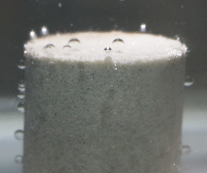
Another example of an early vaporization was the water phase change in shale. At a temperature of 76 °C (349.15 K), the first water gas bubble appeared on the surface (figure 16a). Slow formation of bubbles took place at 82 °C (355.15 K), as presented in figure 16(b). A rapid and continuous formation of gas bubbles of water occurred at 84 °C (357.15 K) (figure 16c). Figure 17 presents the temperatures of the three stages of water, heptane and decane in Berea sandstone, Indiana limestone, tight sandstone and shale, including their normal boiling temperatures in the bulk models. The occurrence of phase alteration in fluids highly depends on the random motion of molecules due to the change of their energies. As a result, the actual boiling stage might happen at any temperature between the first and third stage. In all the cases, the third stage was treated as the boiling temperature of the liquid. Although considering the third stage as the boiling phase of the liquid could result in overestimated boiling temperatures, taking such consideration brought pessimistic outcomes. In other words, the highest possible temperature value was taken as the bubbling point to avoid any errors caused by experimental error. Even in these circumstances, the values obtained were much lower than those in the bulk conditions as will be discussed in the next sections.

Figure 16. (a) Initial water bubble creation (stage 1) at 76 °C in shale; (b) slow and continuous water bubble formation (stage 2) at 82 °C in shale; (c) rapid and continuous water bubble formation (stage 3) at 84 °C in shale.

Figure 17. Temperatures of the three main stages of water, heptane and decane in Berea sandstone, Indiana limestone, tight sandstone, shale and bulk model.
7.1. Comparison of experimental results with theory (Thomson equation)
According to the Thomson equation (3.2), porous media (capillary condition) can have a significant impact on the boiling points of liquids when the pore radius is less than 1000 nm. Since extended tight pores (smaller than 100 nm) do exist in the permeable rocks, liquids tend to boil in such matrixes at lower temperatures than their normal boiling temperatures. Figures 18 and 19 illustrate the average vaporization temperatures and temperatures of the two reading points (first and third stages) of water, heptane and decane in Indiana limestone, Berea sandstone, tight sandstone, shale and bulk condition. Moreover, the experimental results were compared with computed vaporization temperatures, obtained from the Thomson equation. For the rock samples, average pore-throat sizes, in figure 18, were estimated using the Winland equation and considered to compare the outcomes with the computed vaporization temperatures.

Figure 18. Calculated vaporization temperatures and measured boiling points of heptane, water and decane in bulk case and different rock samples; the average pore size of each rock was computed using the Winland equation. The boiling temperatures were measured under atmospheric pressure (1 atm).

Figure 19. Calculated vaporization temperatures and measured boiling points of heptane, water and decane in bulk case and different rock samples; median pore diameters were considered. The boiling temperatures were measured under atmospheric pressure (1 atm).
Meanwhile, median pore sizes (given in table 2) were considered as another way to represent a single pore size value. These values were calculated by measuring areas under the curves in pore size distribution graphs assuming that pore sizes smaller than 1000 nm dictate the ‘early’ boiling process. This assumption is based on the theoretical observations and the Thomson equation, implying that 1000 nm is the threshold above which the porous structures behave like bulk (see solid lines in figure 18). The results for the median pore size are shown in figure 19. In both average (obtained using the Winland equation) and median pore size cases, the observed vaporization of water, heptane and decane in the rocks took place at temperatures lower than the bulk cases, as shown in figures 18 and 19.
Figure 20 summarizes the results obtained from the Hele-Shaw and microfluidic experiments with heptane, and compares them with the observed outcomes from the rock experiments and computed heptane vaporization temperatures using the Thomson equation. Since the nature of the curved interface is not identified in the silica-glass models and rock porous media, the interfacial tension at the vapour–liquid interface  $({\sigma ^{LV}})$ was assumed to be unaffected by the curvature. Furthermore, it was assumed that the rock molecules were not interfering with the vapour–liquid interface. According to the microfluidic experiments, on average, the reduction of heptane vaporization temperatures, from the bulk condition and computed vaporization point, was 22 % (4.8 % in kelvin unit) in an average pore throat of 15 000 nm (0.015 mm). As a result of the non-curved solid–liquid contact in the Hele-Shaw glass cells, the recorded phase-change temperatures of heptane were nearly 20 % (4.3 % in kelvin unit) lower than those found for the micromodel observations. Generally, the vaporization of heptane in the rocks took place at temperatures lower than the bulk condition by almost 22 % (4.8 % in kelvin unit). The average boiling temperature of heptane (73 °C, 346.15 K) in sandstone, limestone and tight sandstone was 24 % (5.4 % in kelvin unit) below the calculated phase-transition temperature (98 °C, 371.15 K), estimated using the Thomson equation. In shale, the measured heptane boiling point (83 °C, 356.15 K) was noticed to be lower than the computed temperature (93 °C, 366.15 K) by 15 % (3.2 % in kelvin unit). Overall, the outcomes obtained from the rock experiments were consistent with the microfluidic observations, as shown in figure 20.

Figure 20. Measured boiling temperatures of heptane from Hele-Shaw, micromodel and rock experiments and calculated phase-transition temperatures, obtained from the Thomson equation.
8. Sensitivity of bubble point detection
The temperatures of the first, second, and third stages were measured based on the appearance of gas bubbles on the rock surface (figure 14). With the same liquid, the first stage (formation of initial bubbles) was noticed to take place in the rocks at different temperatures. For instance, figure 21 presents the temperatures of the three stages of heptane in the used rock samples. During the first stage, the existence of the first bubbles depends partially on the size of pores. Nonetheless, initial heptane gas bubbles started to appear on the shale's surface at a temperature (72 °C, 345.15 K) that was higher than what was observed in sandstone, limestone, and tight sandstone, although the pores in shale are tighter than the inner channels of the other rocks. The reason behind such a phenomenon was the low permeability of shale, which restricted the movement of gas bubbles within the rock. Similarly, the second and third stage, in shale, occurred at temperatures higher than what were measured in other rocks, due to its tight nature (much lower permeability than other samples).

Figure 21. Temperatures of the three stages of heptane in Berea sandstone, Indiana limestone, tight sandstone and shale.
9. Detailed analysis of bubble point detection in rocks
Bubble generation and nucleation in microfluidic glass models can be visualized promptly due to the transparent nature of the micromodels. Vaporization inside the rock pores, however, cannot be observed unless the bubbles appear on the rock surface. The migration of a bubble from the point of generation to the surface may take a while if the permeability (or pore size) is small. This delay can be attributed to wettability and clay content as well. Hence, further analysis was performed to determine a possible margin of error caused by those factors, and the temperatures at which bubbling started for each rock type were compared.
Figures 22–24 show the temperatures at which the first bubble appeared and continuous bubbling developed in the sandstone, limestone, tight sandstone, shale and bulk model. Characteristically, the first bubble appeared on the tight sandstone compared to other rock types. This makes sense as its permeability (table 1) and median pore size is smaller than 100 nm as well as the volume content in the whole system (table 2) being much smaller than that of the Berea sandstone and Indiana limestone samples.

Figure 22. Bubble point detection temperatures for heptane in sandstone, limestone, tight sandstone, shale and bulk model.
On the other hand, one would expect that liquids should vaporize in shales at a lower temperature than in the tight sandstone as almost all pores are smaller than 1000 nm (table 2 and figure 11) and the average/median pore size of the shale sample is considerably lower than that of the tight sandstone. This might be due to the fact that the ultra-low permeability of shale slowed the motion of the bubbles upward in the rock, leading to the vapour bubbles appearing on the rock surface at higher temperatures than that observed for the other rocks. In other words, in the tight sandstone, water, heptane and decane bubbles appeared on the rock surfaces at lower temperatures than those measured in shale – even though both types of rocks contained a comparable amount of pore sizes smaller than 1000 nm (figure 10). Due to the higher permeability of tight sandstone, the mobility of vapour bubbles in the rock was more than the case in shale, which explains the appearance of water, heptane and decane bubbles on the outer surface of the tight sandstone sample at lower temperatures than observed in shale at the same conditions.
Also, note that the temperatures at which the first bubble was detected for Berea sandstone and Indiana limestone were lower than that for the shale sample for heptane (figure 22) and decane (figure 24) even though both samples are extremely low in pore sizes smaller than 1000 nm (table 2 and figure 11). This can be attributed to the permeability effect, which caused a delay in discharging the bubbles out of the rock in the case of the shale sample.
The above observations are valid for the hydrocarbon solvents (heptane and decane). In the case of water, one may see the effect of permeability on the bubble discharge mechanism but Berea sandstone and Indiana limestone showed a different behaviour compared to the solvent cases. The lowest temperature at which the first bubble appeared was measured for Berea sandstone (figure 23). Indiana limestone showed the highest temperature among all four samples for the detection of the first bubble. These observations could be attributed to another characteristic of capillary medium, wettability, which is controlled by the rock mineralogy and thereby clay content. As a result of rock wettability, certain liquids are held by the inner pore surface, which could be the case for limestone, which shows less water wetting nature. The clay content also plays a role due to higher adsorption capacity, especially for solvents. The solvents have a higher tendency to be adsorbed onto clays, and Berea sandstone shows high clay content. The effect leads to stronger surface-molecule forces, which require more thermal energy or higher temperatures to break them. In the case with heptane (figure 22), however, the formation of the first bubbles on the sandstone surface was noticed at the identical temperature to that for tight sandstone. Despite the low volume percentages of pores below 1000 nm in sandstone and limestone (table 2), their existence could result in early vaporizations at temperatures similar to what was observed with tight sandstone.

Figure 23. Bubble point detection temperatures for water in sandstone, limestone, tight sandstone, shale and bulk model.
The results obtained with the bulk model were used as benchmarks and comparisons made with the temperature values obtained with the rocks and, despite all the uncertainties described above, one may observe that the lowest and highest temperatures taken as the indicator of boiling (first bubble appearing and continuous boiling, respectively) are still considerably lower than that of the bulk case as can be observed in figures 22–24. In other words, the nucleation temperatures in sandstone, limestone, tight sandstone and shale were lower than those detected in the bulk model, owing to the confinement effect in the rocks.

Figure 24. Bubble point detection temperatures for decane in sandstone, limestone, tight sandstone and shale.
10. Conclusion and remarks
By performing microfluidic and rock sample experiments, boiling temperatures of water and several hydrocarbon solvents were investigated in confined capillary/porous media. Then, the experimental observations were compared with the calculated vaporization temperatures, obtained from the Thomson equation. The conclusions can be listed as follows:
(i) The microfluidic experiments showed that the boiling temperatures of heptane, heptane–decane mixture and naphtha decline by 20 % (4.3 % in kelvin unit) approximately with the reduction of medium size.
(ii) Although the volume percentages of micropores (≤2 nm) and mesopores (2–50 nm) were less than 5 % in Berea sandstone and Indiana limestone, the presence of such pores resulted in early vaporizations of water, heptane and decane, as observed in figure 17.
(iii) Due to the considerable volume percentages of extended nanopores (≤100 nm) in shale and tight sandstone, noticeable reductions of water, heptane and decane vaporization temperatures by nearly 18 % (3.8 % in kelvin unit) were observed.
(iv) At a reservoir scale, such reductions of boiling temperature could have a considerable impact on history matching and performance forecasting for oil, gas and geothermal production, especially in tight reservoirs.
Acknowledgements
This research was conducted under the second author's (T.B.) NSERC Industrial Research Chair in Unconventional Oil Recovery (industrial partners are Petroleum Development Oman, Total E&P Recherche Development, Husky Energy, Saudi Aramco, CNRL, Suncor and BASF) and an NSERC Discovery Grant (no. RES0011227). We gratefully acknowledge this support. The first author (I.A.-K.) is grateful to Petroleum Development Oman Co. (PDO) for providing financial support for his graduate study at the University of Alberta.
Declaration of interests
The authors report no conflict of interest.


