


Spatial theories of voting presume that voters reduce a candidate’s platform to an ideological position.Footnote 1 This ideological position captures how the voter believes that the candidate will, if elected, affect policy outcomes.Footnote 2 In most theories of electoral competition, voters presume that the platform of the winning candidate will be the policy that is implemented after the election. This is a convenient and productive simplification but it is not an innocuous one, particularly when considering the role of most elected officials: few, if any, political offices in a democracy allow the officeholder to unilaterally impose his or her will by fiat. Rather, the official must work through an institutionalized process in order to have some effect on public policy.Footnote 3
In this article, we focus on a near-ubiquitous characteristic of policymaking processes: the menu of choices from which a representative may choose is at least partially determined by actors and/or events beyond the representative’s control. Put differently, most officials with decision-making authority spend most of their time making decisions about issues and between choices that were chosen by someone else. Both internal procedures and external events, such as disasters, force policymakers to choose between options other than their most-preferred policies.Footnote 4 Examples include a legislator who may implement a “platform” only through voting on bills that are not necessarily representative of the policies that he or she would implement if given unilateral authority; an executive who may only sign or veto legislation passed by a legislature; or a judge who may only make decisions on cases brought by others.
We explore the implications of this reality for a voter evaluating various candidates’ platforms. Specifically, we consider a voter with an ideological position (v ∈ R) and derive the voter’s expected payoff from a candidate with a known platform (p ∈ R).Footnote 5 The candidate chosen by the voter will then be faced with a pair of options to choose from, and will pick the option closest to his or her platform. Unsurprisingly, the voter’s expectations about the options the representative will confront affect how the voter evaluates competing ideological platforms.
The central point of this article is as follows: when representatives may be faced with an exogenous set of options to choose from, voter preferences for candidate platforms do not look like voter preferences for policy. In particular, the voter’s evaluation of candidate platforms becomes asymmetric about the voter’s own ideal position even if his or her policy preferences are symmetric. We show that, in a variety of choice environments, these expectations induce a strict preference on the part of the voter for more extreme candidates.
Our notion of extremity is relative to both the voter’s own preferences and what we term the legislative agenda: the distribution of options that the representative is likely to be choosing from. For example, as we discuss in more detail below, if the voter tends to be (say) to the right of the alternatives likely to be brought up as potential choices, then a more extreme candidate is one whose platform is to the right of the voter’s ideal policy position.
A key finding from our theory is that when a voter believes that the legislative agenda is ideologically distant from his or her own position, a voter considering two platforms equidistant from his or her own ideal point will prefer the platform farther from the legislative action to the platform closer to it. While this induced “taste for extremism” can be reversed for some voters under some circumstances,Footnote 6 there will always exist voters with a taste for extremism. On the other hand, there may exist no voters with a taste for moderation—voters who prefer the platform closer to the center of the legislative agenda.
ASYMMETRIC PREFERENCES AND VOTING
In terms of the causal mechanism at the heart of our theory, our paper is most closely related to Grofman (Reference Grofman1985), who discusses the role of the status quo in spatial models of voting. Grofman identifies a problem similar to our starting concern: that candidates are limited in their ability to implement their platforms. He focuses on the status quo as representing a starting point for policy change, and develops a model in which a voter does not care directly about party platforms but about the outcomes the voter thinks each party is capable of achieving.
Grofman’s model generates two insights that we also identify, for related reasons. First, voter preferences over candidate platforms may change over time even when those platforms remain unchanged. And second, it is not always advantageous for a candidate to be thought able to implement his or her platform; a very extreme but incapable candidate may be successful precisely because he or she moves the status quo in the right direction but not too far. In Grofman’s model, both of these insights are consequences of the location of the status quo and how parties are assumed to shift policy from this point. In our model they stem from the voter’s perception of the choices the candidate is likely to encounter. The main, and crucial, distinction between these two models is that we remain firmly grounded in the spatial model of choice. In our model there are only voter ideal points, candidate platforms, and choices likely to be encountered by candidates. If two candidates will always vote the same way then the voter is indifferent between them, regardless of their platforms.Footnote 7 In contrast, Grofman presents a directional model of party behavior in which the party is capable of implementing a weighted measure of its platform.
Grofman’s approach is similar to the coalition bargaining mechanism in Kedar (Reference Kedar2005, Reference Kedar2009) and, accordingly, Kedar’s theory offers some conclusions that are similar to ours.Footnote 8 However, as with Grofman’s theory, Kedar’s conclusions are generated by a different causal mechanism. Specifically, as with Austen-Smith and Banks (Reference Austen-Smith and Banks1988), voters’ vote choices can affect the legislative agenda (i.e., the set of policies from which the legislators can choose), and voters’ induced preferences for representatives take this into account. In our model, the voter’s vote choice can affect only how his or her representative will vote: the agenda is exogenous.
As with both Grofman (Reference Grofman1985) and Kedar (Reference Kedar2005), our theory suggests one way to at least partially understand conflicting empirical results regarding proximity and directional voting models (e.g., Rabinowitz and Macdonald Reference Rabinowitz and Macdonald1989; Platt, Poole, and Rosenthal Reference Platt, Poole and Rosenthal1992; Lewis and King Reference Lewis and King1999; Adams, Merrill III, and Grofman Reference Adams, Merrill and Grofman2005; and Tomz and Van Houweling Reference Tomz and Van Houweling2008). Specifically, the empirical predictions of our theory of voting are sometimes in line with those of the proximity model and sometimes in line with the directional model. For example, according to our theory, voters confronted by two platforms on the same side of their ideal point will vote for the closest platform, in line with proximity models of voting. On the other hand, if the voter is choosing between two platforms on opposite sides of his or her ideal point the voter’s best choice will sometimes be the platform that is on the opposite side of the voter’s ideal point from the status quo (or “neutral point”), as predicted by the directional theory of voting.Footnote 9
THEORIES OF DELEGATION
While we frame our analysis and presentation in terms of voters choosing between different candidates, our framework can be viewed more generally as a theory of delegation. In this vein, it is useful to connect our findings with, and distinguish our logic from, those of the broader literature. For example, it is well-known that many agency problems generate incentives for a principal to choose an agent whose preferences differ from his or her own. This is a central theme within models of “strategic delegation.”Footnote 10 While our theory generates insights that are compatible with those derived within this literature, the logic of our theory is different. Specifically, strategic delegation arguments indicating that a principal’s preferences over agents differ from his or her preferences over outcomes rely upon either the strategic interaction of multiple agents or asymmetric information between the principal and the agent.
In such situations, the principal’s preference derives either from the fact that the agent will influence the strategic behavior of third-party actors in ways that benefit the agent, or from the fact that—in the presence of asymmetric information—preference divergence between a principal and agent may induce beneficial behavior (e.g., ameliorate shirking) by the agent. In contrast, we assume that the voter cares only about how his or her representative will sincerely choose from an exogenous slate of policy choices.Footnote 11 Thus, the divergence in voter preferences for policies and platforms that we identify is based solely on unilateral and sincere behavior on the part of the representative.
A Roadmap
In the remainder of the paper we first set up our model of voter choice, present a few general insights that fall out of the model, and explore two settings that provide intuition for our finding that a relative preference for more extreme, rather than more moderate, platforms will emerge when voters choose a representative to choose on their behalf. Following that, we present two applications of our theory to well-known models of electoral politics: Downsian competition and Osborne and Slivinsky’s “citizen-candidate” model.Footnote 12 In both settings, we find that electoral competition will generate more extreme platforms than is predicted when, as is traditionally done, voters are assumed to have symmetric preferences over candidates’ platforms. Finally, we conclude with a discussion of how our theory is related to existing theories of delegation and voter choice, including the literature comparing the proximity and directional theories of voting.
THE MODEL
We consider a model of voting between candidates with policy platforms in a unidimensional policy space X ⊆ R and denote the set of voters by N = {1, …, n}. We characterize each voter i by his or her ideal point, v i ∈ R, and denote the median of the ideal points by v m.Footnote 13
Voters’ Policy Preferences
Each voter i’s policy preferences are represented by a real-valued policy payoff function u : R2 → R where u(x, v i) denotes the payoff received by voter i if policy x is chosen. In order to highlight the asymmetric preferences our model induces, we assume that u is symmetric about the voter’s ideal point:
 $$u\left( {x,v} \right) = u\left( {y,v} \right) \,\Leftrightarrow\, \left| {x - v} \right| = \left| {y - v} \right|.$$
We also assume that the function u satisfies increasing differences. This means that for x > y, u(x, v) − u(y, v) is weakly increasing in v. All of our assumptions are consistent with most commonly used functional forms, including linear loss and quadratic loss.
Candidates’ Platforms
Any candidate, c, is characterized by his or her platform, p c ∈ X. If elected, candidate c’s platform, p c, will determine the candidate’s subsequent voting behavior as follows. For any pair consisting of a bill and status quo, (q, b), a candidate with platform p c will vote for the bill, b, if and only if u(b, p c) > u(q, p c). That is, any candidate c would vote as the voter would vote if the voter had ideal point equal to p c. For any platform p c, this voting behavior is represented formally by the following function:
 $$V\left( {b,q,{p_c}} \right) = \left\{ {\matrix{ b \hfill & {{\rm{if}}\;u\left( {b,{p_c}} \right) > u\left( {q,{p_c}} \right),} \vskip8pt\hfill \cr q \hfill & {{\rm{otherwise}}{\rm{.}}} \hfill \cr} } \right.$$
The Agenda
We conceive of a legislative agenda that describes the likelihood that different (q, b) pairs will arise. To capture the idea that the voter is choosing a platform to represent his or her interests in the face of an exogenous agenda, we represent the agenda as a probability measure, α, over X 2. We consider two specific representations of the agenda in the body of the article and present a generalization allowing for the agenda to be partially endogenous in Online Appendix E. Prior to that, we summarize our theory of voter choice and establish a few general results.
PREFERENCES OVER PLATFORMS
Viewed at its most general, our theory of voter choice is that the voter votes for (or selects) the candidate whose platform maximizes the following expected payoff function:
 $$EU\left( {p,v} \right) = \int_{{X^2}} {u\left( {V\left( {b,q,p} \right),v} \right){\rm{d}}\alpha } .$$
In order to simplify presentation, we assume here that a voter’s expected payoff from a candidate with platform p is his or her expected utility from a policy the candidate will vote for. That said, Equation (1) is flexible and represents a variety of scenarios, including both instrumental and expressive motivations on the part of the voter. We now briefly describe each of these two possible interpretations for Equation (1).
Instrumental Motivations
If we suppose that the representative is always decisive (i.e., that the alternative he or she chooses is actually implemented as policy), then the theory of voter preference over platforms expressed in Equation (1) is clearly instrumental. However, if the voter’s chosen representative influences policy only indirectly (for example, as a member voting within a larger legislature), then Equation (1) neglects the details of how the representative’s choice will influence the institution’s ultimate decision. Specifically, Equation (1) does not consider the probability that any given platform p will cast a decisive vote in the larger legislature. In Online Appendix D, we show that our results carry through in an extended setting with multiple legislators and the voter’s expected payoff from a platform p is based purely on “instrumental” considerations and is a function of the probability (which depends on the composition of the legislature) that the legislator’s vote will be pivotal.
Expressive Motivations
Of course, regardless of the institutional setting, a simple interpretation of Equation (1) is as representing “expressive” preferences.Footnote 14 Within such an interpretation, Equation (1) directly represents the voter’s desire to support candidates whose voting behavior would maximize the voter’s payoff if those votes were converted into actual policy, regardless of whether or how those votes actually influence the implemented policy.
CHOOSING BETWEEN PLATFORMS
We can describe the voter’s expected payoff function in some detail without specifying the agenda, α. To do so, we first introduce the notion of “disagreement sets.” The disagreement set between a voter with ideal point v and a candidate with platform p is the set of bill/status quo pairs on which the candidate’s vote would differ from how the voter would vote:
 $$\displaylines{ D\left( {p,v} \right) \,\equiv \,\left\{ {\left( {q,b} \right):V\left( {b,q,p} \right) \ne V\left( {b,q,v} \right)} \right\},\;{\rm{or}} \cr = \left\{ {\matrix{ {\left\{ {\left( {q,b} \right):2p - q \,\lt b \,\lt \,2v - q} \right\}} & {{\rm{if}}\;p \,\lt \,v} \cr {\left\{ {\left( {q,b} \right):2p - q > b > 2v - q} \right\}} & {{\rm{if}}\;p > v.} \cr} } \right. \cr}$$
Figure 1 illustrates this idea. The left panel of Figure 1 displays the voter’s preferred vote choice for every possible pair of status quo, q, and bill, b, and the right panel of the figure displays the disagreement set for a voter with ideal point v and a candidate with platform p.

FIGURE 1. Voter Preferences Over Votes (left) & Voter-Candidate Disagreement Set (right)
We start with an intuitive lemma that several of our results follow from. This lemma says that if the disagreement set for v and p 1 is a subset of the disagreement set for v and p 2, then a voter with ideal point v receives a weakly higher expected payoff from p 1 than p 2. All proofs for this section are relegated to Appendix A.
Lemma 1. If D(p 1, v) ⊆ D(p 2, v) then EU(p 1, v) ≥ EU(p 2, v).
The following theorem is a direct corollary of Lemma 1, and is presented without proof. It states that a voter’s expected payoff is maximized (though perhaps not uniquely) by a representative whose platform is equal to the voter’s ideal point. This is because the disagreement region between a voter and platform p = v is empty.
Theorem 1. For any ideal point v ∈ X and any agenda α, the function EU(p, v) is maximized at p = v.
The next theorem extends Theorem 1 by establishing that the expected payoff function is single-plateaued. Thus, as platforms move to either the left or right of the voter’s ideal point, the voter’s expected payoff weakly decreases. It is proved by showing that disagreement sets are nested as platforms move away from v in one direction.
Theorem 2. For any ideal point v ∈ X and any agenda α, the function EU(p, v) is single plateaued: if p  $\le p \,\le\, v$ then
  $EU\left( {{\b{p}},v} \right) \,\le \,EU\left( {p,v} \right)$ and, if
  $\bar{p} \,\ge p \,\ge \,v$ then
  $EU\left( {\bar{p},v} \right) \,\le \,EU\left( {p,v} \right)$.
Theorems 1 and 2 jointly establish a weak version of the “ally principle” (Bendor and Meirowitz Reference Bendor and Meirowitz2004) in this setting. Theorem 1 establishes that each voter should, if possible, appoint his or her ideological clone to vote on his or her behalf. Theorem 2 goes a step farther and implies that, when choosing among candidates whose platforms are all on the same side of the voter’s ideal point then the voter should appoint the candidate whose platform is closest to his or her ideal point. These establish only a “weak version” of the ally principle because they do not imply that “all else equal, a rational boss should choose her closest ally as an agent.”Footnote 15 Specifically, Theorems 1 and 2 do not address situations in which the two candidates offer platforms on opposite sides of the voter’s ideal point.
Our final result in this section establishes that the family of voter expected utility functions satisfies a single-crossing condition. This result is important because it establishes that there exists an individual whose voting behavior is equivalent to the majority preference relation for any binary vote that could occur. This ensures that the median voter is a “representative voter” when we apply our model to Downsian and citizen-candidate models of electoral competition.Footnote 16
Theorem 3. The median voter is a representative voter over platforms: a majority of the voters in N prefer a platform p over platform p′ if and only if the median voter prefers p over p′.
With Theorem 3 in hand, we will drop the m subscript and simply write the median voter’s ideal point as v ≡ v m as long as the context is clear. We now turn to imposing some more structure on the agenda, α, beginning with a clear baseline that we refer to as the symmetric agenda case.
SYMMETRIC AGENDAS
Our central result—an induced preference for relatively extreme platforms over relatively moderate ones—is most clearly presented by focusing attention on agendas that satisfy an independence and symmetry requirement. We formally define these requirements in Appendix A (Definitions 3 and 4). For our purposes here, an agenda α is symmetric around (μ b, μ q) if it can be expressed as a probability distribution with a continuously differentiable and strictly quasi-concave probability density function with circular isodensity curves centered on (μ b, μ q) ∈ R2.Footnote 17 This is satisfied if b and q are independent Normal(μ b, σ 2) and Normal(μ q, σ 2) random variables for any given σ > 0.
Defining Extreme and Moderate Platforms
In our model, voter preferences for a candidate are determined solely by the candidate’s platform and the legislative agenda. Consequently, our notion of extremism is indirect in that we define it solely in terms of platforms and agendas. In other words, we consider candidate extremism relative to the legislative agenda α, conceiving of the agenda as a proxy for political climate. Formally, our definition of moderation/extremity of platforms is stated in Definition 1 and illustrated in Figure 2.

FIGURE 2. Moderation & Extremism of Platforms Relative to the Agenda
Definition 1. For any agenda α that is symmetric about (μ b, μ q), platform is more moderate relative to α than platform p 2 if p 1 is closer to the midpoint between μ b and μ q than is p 2:
 $$\left| {{p_1} - {{{\mu _b} + {\mu _q}} \over 2}} \right| \,\lt \,\left| {{p_2} - {{{\mu _b} + {\mu _q}} \over 2}} \right|.$$
When this holds, we refer to platform p 2 as more extreme relative to α than platform p 1.
Figure 2 depicts a bill distribution centered at μ b and a status quo distribution centered at μ q. The platform on the right, p 1, is more moderate than the platform on the left, p 2, because it is closer to the “center” of the agenda, defined as the midpoint of μ b and μ q.
A Taste for Extremism
The focus of this article is on asymmetries in voter preferences over representatives’ platforms. Asymmetric preferences over platforms are identified by comparing platforms that are equidistant from, and on opposite sides of, the voter’s ideal point. Specifically, for any given divergence from the voter’s ideal point, δ > 0, and comparing two platforms that are equidistant from v (platforms p R = v + δ and p L = v − δ), when does the voter strictly prefer the extremist candidate to the moderate candidate or vice versa? If, whenever one of these candidates is more extreme than the other it follows that the voter strictly prefers the extreme candidate to the moderate candidate, then we say that the voter has a taste for extremism.
Definition 2. Let p L = v − δ and p R = v + δ for some δ > 0. For any agenda α, a voter with ideal point v has a taste for extremism at δ if p L more extreme than p R implies that EU(p L, v) > EU(p R, v) and if p R more extreme than p L implies that EU(p R, v) > EU(p L, v).
It is important to note that—even if the voter has a taste for extremism at all δ—Definition 2 does not imply that for any two candidates a voter with a taste for extremism prefers the extreme candidate to the more moderate one. In particular, single-plateauedness of the voter’s expected payoff function (Theorem 2) always implies that if v is more moderate than platform p, with p > v for example, then the voter (weakly) prefers all platforms on the interval [v, p) to platform p. Our definition only compares platforms equidistant from v. We now provide a simple example of what induced voter preferences over platforms look like with a symmetric agenda, α.
Example 1. Let the agenda α be the bivariate Normal distribution with mean (0, 0) and variance-covariance matrix equal to the identity matrix. Thus, the pairs of alternatives are independently and identically distributed according to the Normal(0, 1) distribution. The following figures depict the preferences of a voter with ideal point v = −0.3. The utility function on the left displays the voter’s preference for policy, and that on the right illustrates his or her induced preference for platforms, given the agenda α.
Figure 3 shows that a voter whose ideal policy v is to the left of the “center” of the legislative agenda has preferences that favor a leftward deviation from v over an equally sized rightward deviation from v. This preference for extremism for a given value of δ is indicated on the right panel of Figure 3: the expected utility from platform p L = v − δ is strictly higher than that from p L + δ.
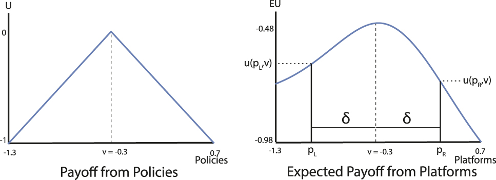
FIGURE 3. Preferences for Policies Versus Preferences for Platforms
The following results establish that the voter has a taste for extremism for all values of δ > 0 when the agenda is symmetric.
Theorem 4. For any agenda, α, that is symmetric around (μ b, μ q) and any δ > 0, the voter strictly prefers left candidate p L = v − δ if and only if  $v \,\lt {{{\mu _b} + {\mu _q}} \over 2}$ and strictly prefers right candidate p R = v + δ if and only if
  $v > {{{\mu _b} + {\mu _q}} \over 2}$.
Theorem 4 implies that, when agendas are symmetric, nearly every voter has a taste for extremism. This is stated in the following corollary.
Corollary 1. When α is symmetric, every voter with  $v \ne {{{\mu _b} + {\mu _q}} \over 2}$ has a taste for extremism.
The intuition behind Theorem 4 and Corollary 1 is displayed in Figure 4, which shows the disagreement sets between v and p L (the darker trapezoid) and v and p R (the lighter one). A contour plot of an agenda that draws pairs centered to the right of (v, v) is shown, representing the bivariate normal distribution we have assumed. Since p R is closer to the center of legislative activity, it is more likely that a vote will be drawn on which the voter and R disagree. As the figure shows, agenda α assigns greater mass to policy pairs on the voter and R’s disagreement set than on the voter and L’s. Put differently, L is a “safer” candidate for the voter precisely because he or she is more extreme relative to the agenda.

FIGURE 4. Intuition for Voter Preference for Extremism
We now turn to consider a more detailed conception of the agenda process in which one policy, the “status quo,” is known and the only uncertainty about the agenda is the location of the other (i.e., the “bill”).
AGENDAS WITH ONE FIXED ALTERNATIVE
It may be natural to consider the symmetric agenda environment described in Theorem 4 when choosing a delegate (such as a judge or bureaucrat) to adjudicate disputes that arise exogenously. In such cases we may wish to incorporate uncertainty about both options that the appointed representative will be choosing between. However, the standard spatial bargaining framework utilized by political economy scholars for the past 40 years typically assumes a status quo that is fixed and known to the voter.Footnote 18 In addition to comparability with existing scholarship, the assumption of an exogenous and known status quo is the most parsimonious way to consider “asymmetric” agendas.Footnote 19 Here, we present some results when the status quo policy is fixed and normalized to equal zero (i.e., q = 0 with certainty). The voter’s uncertainty about the vote that the elected representative will face is then solely with respect to the location of the bill, b. We assume that the distribution of bills is described by a symmetric and quasi-concave probability density function, f : R → R, with cumulative distribution function, F. We denote the mode of f by μ b.Footnote 20 In this setting, the expected payoff for a voter with ideal point v from a candidate with a platform equal to p is
 $$EU\left( {p,v} \right) = \int_X {u\,\left( {V\left( {b,0,p} \right),v} \right)\,f\left( b \right){\rm{d}}b} .$$
This is simply the voter’s expected utility for a vote between status quo q = 0 and a bill distributed according to f, taken by a candidate with platform p. For reasons of space, we limit our discussion to the case in which candidate divergence about the voter’s ideal point, δ, is small relative to v, or v ≥ 2δ. The remaining cases are presented in Appendix B. We also assume throughout this section that v > 0 (which is without loss of generality), and that the voter’s payoff function is the linear loss function:
 $$u\left( {p,v} \right) = - \left| {p - v} \right|.$$
The Voter’s Incentives in the Known Status Quo Case
To understand the incentives in the known status quo model, note that there is a single interval of bills on which the two platforms, p L = v − δ and p R = v + δ will vote differently from each other. Specifically, when b < 0 then both candidates and the voter prefer the status quo q = 0 to the bill b and when 0 < b < 2p L, both candidates and the voter prefer the bill b to the status quo q = 0. Similarly, when b > 2p R then both candidates and the voter prefer the status quo to the bill. We can therefore restrict attention to the interval [2p L, 2p R]; for any bill drawn from this interval the preferences of the two candidates diverge. As before, we call this interval the disagreement set for the known status quo setting.
Figure 5 shows the disagreement set when candidate divergence is small relative to the voter’s ideal point (2δ ≤ v). This figure also depicts the difference in the voter’s expected utility calculation for R’s vote over L’s vote for each possible bill, or u(V(b, 0, p R), v) − u(V(b, 0, p L), v). Using Definition 1 of extremism presented in the previous section, this implies the right candidate (v + δ) is extreme when μ b < 2v and the left candidate (v − δ) is extreme when μ b > 2v.
FIGURE 5. Disagreement Region when  $\bolddelta \,\boldle \,{\bi{v \over 2}}$
When p L ≥ 0, or equivalently, δ ≤ v, the left candidate will always vote for status quo q = 0 and the right candidate will always vote for bill b on the entire disagreement region. The voter prefers the bill on [2p L, 2v] and prefers the status quo on [2v, 2p R]. To consider a voter’s taste for extremism over moderation (Definition 2), first note that when  ${p_L} > {v \over 2}$ (or phrased alternatively, when v ≥ 2δ) the entire disagreement region lies to the right of v; in this case, b ≥ v for all b in the disagreement region. Let ΔU (p 1, p 2) ≡ EU (p 1, v) − EU (p 2, v). Then,
 $$\Delta U\left( {{p_R},{p_L}} \right) = \int_{2{p_L}}^{2{p_R}} {\left( { - \left( {b - v} \right) + v} \right)} \,f\left( b \right){\rm{d}}b,$$
or
 $$\Delta U\left( {{p_R},{p_L}} \right) = \int_{2{p_L} - q}^{2{p_R} - q} {\left( {2v - b} \right)\,f\left( b \right){\rm{d}}b} .$$
 For this case where  ${p_L} \in \left[ {{v \over 2},v} \right)$ (Figure 5) the voter always has a strong taste for extremism; he always prefers R to L when μ b < 2v and prefers L to R when μ b > 2v. This is because the bill distribution places more likelihood on bills arising from the side of the bill distribution that favors the extremist candidate. Additionally, ΔU(p R, p L) is symmetric on the region overall, and so the increased likelihood of a bill being drawn from [2p L, 2v] leads to a preference for the extreme candidate over the moderate. As we discuss in Appendix B, this symmetry is specific to the case we are considering, where 2δ ≤ v.
With this in hand, our first result in this setting is that voters whose ideal points are sufficiently distant from the agenda (|v| sufficiently large) prefer the extreme candidate.
Proposition 1. For any level of candidate divergence about the voter’s ideal point, δ > 0, the voter prefers the extremist candidate whenever v ≥ 2δ.
This result can also be interpreted as saying that if the two candidates equidistant from any voter are sufficiently close  $\left( {\delta \le {v \over 2}} \right)$ then the voter always prefers the extreme candidate. Of course, Proposition 1 provides only a sufficient condition for a voter to prefer an extreme candidate: depending on the distribution of bills, f, the voter may prefer the moderate or the extreme candidate when v < 2δ. The exact conditions determining this preference are somewhat cumbersome, and are therefore relegated to Appendix B. However, we can state the following sufficient condition for a taste for moderation.
Proposition 2. For any voter with ideal point v > 0, suppose that b ∼ N(μ b, σ 2). For any level of candidate divergence δ about v such that δ > v, the voter prefers the moderate candidate for sufficiently large values of σ 2 > 0.
The central point of Propositions 1 and 2 is that, when the agenda is not symmetric, a voter’s taste for extremism or moderation depends on the divergence between p L and p R, and on the mass that the distribution of bills, f, assigns to policies on the extreme side of the voter’s ideal point. Loosely put, when the distribution of the bills is sufficiently disperse that bills more extreme than the voter are very likely, then the voter will prefer moderation when considering two equidistant and sufficiently divergent candidates. This is because bills on the far right of the disagreement set yield higher disutility for the extremist candidate than bills on the far left do for the moderate candidate (and this fact is discussed in greater detail in Appendix B). It is the combination of these two conditions, a sufficiently disperse distribution of bills and sufficiently divergent candidate platforms, that reflects the general idea that a taste for moderation is less common than a taste for extremism. We conclude this section with an illustration of the fact that in the known status quo case voters may have a taste for either extremism or moderation, even when the distribution of bills is symmetric.
Example 2. Let the distribution of bills be N[0.2, σ] and fix the status quo at q = 0. Figures 6 and 7 depict the induced preferences of a voter with ideal point v = 0.5 for bill distributions with different variances (the distributions of bills are pictured on the right); in Figure 6 the variance of the bill distribution is σ = 1 and in Figure 7 the variance is σ = 10.
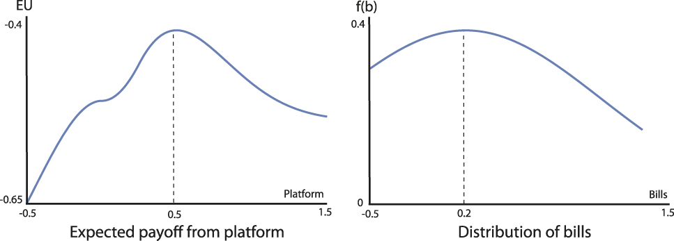
FIGURE 6. Preferences for Platforms with Low Bill Variance
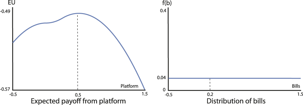
FIGURE 7. Preferences for Platforms with High Bill Variance
In both figures the voter has a taste for the extreme, rightmost candidate for sufficiently small candidate divergence (δ ≤ 0.25, as Proposition 1 tells us). However, when the bill distribution is sufficiently dispersed, as in Figure 7, the voter has a taste for the moderate leftmost candidate as the candidates diverge. When δ = 1 the voter prefers R to L (or platform p R = 1.5 to p L = −0.05) when bill variance σ = 1, but prefers L to R when σ = 10. This is due to the high likelihood of an extreme right bill being drawn when the bill variance is high; such a bill would split the voter and the extremist candidate, and would yield a significant negative payoff to the voter.
IMPLICATIONS IN TWO CANONICAL SETTINGS
We now turn to the implications of asymmetric preferences and a taste for extremism for two classical models of electoral competition: a model of 2-candidate competition between vote-seeking candidates with a little uncertainty (e.g., Downs Reference Downs1957) and a “citizen-candidate” model with endogenous entry by policy-seeking candidates (e.g., Osborne and Slivinsky Reference Osborne and Slivinsky1996; and Besley and Coate Reference Besley and Coate1997). In both of these settings, asymmetry in the voter’s utility function alters well-known predictions about the equilibrium platforms that will emerge in electoral competition.
In the Downsian setting, our framework extends a long-standing literature examining why office-motivated candidates and/or parties might offer divergent platforms when voters have single-peaked preferences.Footnote 21 We are certainly not the first to offer a rationale for divergence. Rather, our contribution adds yet another rationale: asymmetric voter preferences induced by an exogenous agenda.Footnote 22
Two Vote-Seeking Candidates
Here we consider a (nearly) classic model of Downsian competition: two vote-seeking candidates, L and R, compete for the votes of the voters in N. By Theorem 3, this is equivalent to competing for the vote of the median voter, denoted by m ∈ N, with ideal point v m ≡ v.
Let w ∈ {L, R} denote the winning candidate. We tweak the standard framework by incorporating a bit of uncertainty into the process of candidate selection. Specifically, we assume that after the election, but prior to taking office, the winning candidate’s platform, p w, is perturbed to create a realized platform,  $\hat{p}$, as follows:
 $$\hat{p} = {p_w} + \pi .$$
For simplicity we assume that π is distributed Uniform [−ε, ε]. The term ε is an exogenous parameter. From a substantive standpoint, possible sources of perturbations π could include the occurrence of external events with political implications (financial crises, wars, terrorist attacks) or the actions/inducements of other political actors (party leaders, interest groups, donors, activists, the media). The relevant point is that we assume legislators are susceptible to shifts in the ideological leanings of their voting behavior.
Given this uncertainty about each candidate’s realized platform, the median voter’s expected payoff from a candidate with platform p is
 $$\bar{U}\left( {p,v;\varepsilon } \right) \,\equiv \,{\left( {2\varepsilon } \right)^{ - 1}}\int_{ - \varepsilon }^\varepsilon {EU\left( {p + \pi ,v} \right){\rm{d}}\pi } ,$$
and we define
 $$\bar{U}\left( {p,v;0} \right) \equiv \mathop {\lim }\limits_{\varepsilon \to 0} \bar{U}\left( {p,v;\varepsilon } \right) = EU\left( {p,v} \right).$$
 In equilibrium, the candidates each seek to maximize  $\bar{U}\left( {p,v;\varepsilon } \right)$, so that their positions converge to
  $p_L^* = p_R^* = {p^*}\left( \varepsilon \right)$. This is characterized in the following proposition. The proof for this, and all numbered results in this Section, are contained in Appendix C.
Proposition 3. Fix any ε ≥ 0 and suppose that two purely vote-seeking candidates compete for the votes of N voters with ideal points v = {v i}i∈N and unique median m. The unique equilibrium involves both candidates choosing p L = p R = p*(ε), where
 $${p^*}\left( \varepsilon \right) = \mathop {{\rm{argmax}}}\limits_{p \in {\bf{R}}} \bar{U}\left( {p,v;\varepsilon } \right).$$
Furthermore, for any fixed median ideal point v, the function p* : R+ → R satisfies the following four conditions:
1. p*(ε) is located such that the median voter is indifferent between the endpoints of the support of the distribution of π, so that
 $$EU\left( {{p^*} - \varepsilon ,v} \right) = EU\left( {{p^*} + \varepsilon ,v} \right),$$
2. The median voter is perfectly represented when there is no uncertainty, so that
 $${p^*}\left( 0 \right) = v,$$
3. Call the expected payoff function of the median voter right asymmetric if
 $$\delta > 0 \,\Rightarrow \,EU\left( {v + \delta ,v} \right) > EU\left( {v - \delta ,v} \right).$$
If the median voter’s expected payoff function is right asymmetric then p*(ε) > v. Footnote 23
Proposition 3 is illustrated in Figure 8. The figure shows a right-asymmetric expected payoff function (generated from a symmetric N(0, 1) agenda, as in Example 1). Candidates converge to the platform p* that maximizes the expected utility of the median voter. This platform is located at the center of an interval of size 2ε such that the voter’s expected utility function assigns equal values to the two endpoints of the interval. As ε approaches zero, the equilibrium platform, p*(ε) converges to v and, because of the right-asymmetry of the expected utility function, p*(ε) moves farther rightward as ε grows.
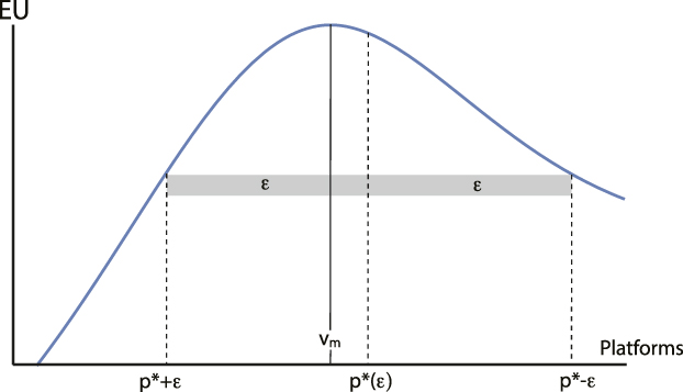
FIGURE 8. Convergent Two-Candidate Equilibrium, p*(ε)
A Citizen-Candidate Model
We now consider a citizen-candidate model in which there is a continuum of voters whose ideal points are uniformly distributed between v min and v max, with v min ≥ 0, v max ≤ 1, and  ${v_m} \,\equiv\, {{{v_{\min }} + {v_{\max }}} \over 2}$. The policy payoffs for a voter with ideal point v i are assumed to be given by the linear loss function:Footnote 24
 $$u\left( {x,{v_i}} \right) = - \left| {x - {v_i}} \right|.$$
Each citizen chooses simultaneously whether to run in the election or not: those who run pay an exogenous and known cost c > 0. Following this, all citizens vote sincerely between the citizens (whose ideal points are assumed to be common knowledge) who chose to run. The winning candidate—determined by plurality rule with fair tie-breaking—chooses sincerely between b and q according to the exogenous agenda, α, based on his or her own ideal point. Finally, we assume that α is symmetric with bills and status quos independently and identically distributed according to the Uniform[0, 1] distribution. The uniform distribution produces expected payoff functions that are strictly single-peaked and qualitatively similar to those produced by the normal distribution (shown in Figure 3). It has the added advantage of being expressible in closed-form, which is characterized in Appendix C.
Summarizing, the timing of the game is as follows:
1. Each citizen chooses whether to enter the race or stay out, with entering costs c > 0.
2. Each citizen votes sincerely for one of the candidates, with the winner decided by plurality rule.Footnote 25 The winner’s platform is denoted by v w.
3. A bill, b, and status quo, q, are each independently drawn from the Uniform[0, 1] distribution.
4. The winning citizen, w, chooses between b and q according to V(b, q, v w).
5. Each citizen receives payoff of u(V(b, q, v w), v i) if they did not run for election and u(V(b, q, v w), v i) − c if they did run for election.Footnote 26
We refer to this model as the Exogenous Agenda Citizen Candidate Model.
Two-Candidate Equilibria
In a pure-strategy, two-candidate equilibrium, the median voter must be indifferent between both candidates’ platforms,  $v_L^*$ and
  $v_R^*$, and these platforms must be located on opposite sides of the median voter’s ideal point, v m. Our first result characterizes pure strategy two candidate equilibria and, most importantly, establishes that these equilibria will inherit the asymmetry of the median voter’s expected payoff function: the extreme candidate’s ideal point will be farther from the median voter’s ideal point than will be that of the moderate candidate.
Proposition 4. In any pure strategy two candidate equilibrium in the Exogenous Agenda Citizen Candidate Model,  $\left( {v_L^*,v_R^*} \right)$,
1.
 $v_L^*$ and $v_R^*$ are located on opposite sides of the median voter’s ideal point, v m $\left( {v_L^* \le {v_m} \le v_R^*} \right)$, and the median voter is indifferent between them:


 $$EU\left( {v_L^*,{v_m}} \right) = EU\left( {v_R^*,{v_m}} \right),$$
2. If the median voter m’s expected payoff function is right asymmetric, then
$v_R^* - {v_m} > {v_m} - v_L^*$. Footnote 27

Empirical Predictions
Any two-candidate equilibrium,  $\left( {v_L^{\rm{*}},v_R^{\rm{*}}} \right)$, can be characterized by two factors: its divergence, which is measured simply by the distance between
  $v_R^*$ and
  $v_L^*$, and what we refer to as its net extremism,
  $\nu \left( {v_L^*,v_R^*,{v_m}} \right)$, which is defined for any pair of platforms, v L ≤ v R, and median voter ideal point v m, as follows.Footnote 28
 $$\nu \left( {{v_L},{v_R},{v_m}} \right) \equiv \left\{ {\matrix{ {{v_R} + {v_L} - 2{v_M}} & {{\rm{if}}\;{v_m} \,\ge \,{1 / 2},} \cr { 2{v_M} - {v_R} - {v_L}} & {{\rm{if}}\;{v_m} \,\le \,{1 / 2}.} \cr} } \right.$$
 The notion of net extremism, ν, measures how much farther away the extremist candidate’s location is from the median voter’s ideal point than is the moderate candidate’s location. Note that, in any two candidate equilibrium in the classical citizen candidate model,  $\left( {v_L^*,v_R^*} \right)$,
 $$\nu \left( {v_L^*,v_R^*,{v_m}} \right) = 0.$$
If there are any two-candidate pure strategy equilibria, there will generally be a continuum of them. Nonetheless, the model generates two additional predictions about equilibria. Specifically, we will focus on the equilibrium with the minimal divergence between the candidates. The first prediction is that the minimal divergence between the candidates in this equilibrium is greater for districts with median voters located farther from the agenda.Footnote 29
Prediction 1. The minimal equilibrium level of divergence, |v R − v L|, is increasing in the distance between the median voter and the agenda, |v m − 1/2|.
Prediction 1 further differentiates the citizen-candidate model in our setting from the classical case, where the minimal level of divergence is constant with respect to the location of the median voter’s ideal point.
The second, related, prediction is that the level of net extremism of the minimal divergence equilibrium is increasing in the distance between the median voter and the agenda, |v m − 1/2|. Along with the asymmetry of the median voter’s expected utility function for all v ≠ 1/2, Conclusion 4 of Proposition 4 establishes that two-candidate pure strategy equilibria will always be characterized by asymmetric platforms, and Prediction 1 establishes that these equilibria become more distant from the median voter’s ideal point as that median voter’s ideal point becomes more distant from the agenda. Prediction 2 complements these conclusions by establishing that the minimal divergence two-candidate equilibrium is “more asymmetric” in the sense that the extreme candidate’s platform is diverging from the voter ideal point faster than is the moderate’s as the median voter’s ideal point diverges from the agenda.
Prediction 2. The level of net extremism of the minimal divergence equilibrium,  $\nu \left( {v_L^*,v_R^*} \right)$, is increasing in the distance between the median voter and the agenda,
  $\left| {{v_m} - {1 / 2}} \right|$.
Predictions 1 and 2 are portrayed in Figure 9. The figure displays, for various locations of the median voter, the minimal divergence two-candidate equilibrium locations for a given cost of entry. As the median voter approaches either end of the spectrum (i.e., becomes more distant from the center of the agenda), the equilibrium locations diverge farther apart (Prediction 1) and the location of the extreme candidate diverges more quickly from the location of the median voter than does that of the moderate candidate (Prediction 2).
FIGURE 9. Effect of Median Voter’s Location on Two Candidate Equilibrium Locations
Viewed from a normative perspective, the predictions are interesting because they imply that the effectiveness of elections to represent the interests of a district’s median voter will depend on the location of the agenda. Proposition 4 implies that competitive elections in more extreme districts—those whose median voters are located farther from the legislative agenda—will be characterized by both more polarized (i.e., ideologically distant) and imbalanced (i.e., the extreme candidate is increasingly farther from the median voter) platforms.
Space precludes a richer treatment of this model (e.g., the question of when elections with more than two candidates will occur is potentially interesting). However, taken together, Proposition 4 and Predictions 1 and 2 demonstrate that the asymmetric preferences generated by our model lead to predictions that are qualitatively different from those generated by standard citizen-candidate models with symmetric preferences.
CONCLUSION
We have presented a theory of voting for representatives that is motivated by a simple question: If policymakers vote according to their platforms, is a voter best off when represented by the policymaker with the platform closest to the voter’s ideal point? Our key finding is that the answer to this question is “no:” a voter’s preferences over candidate platforms will generally differ from his or her preferences over policy. The causal mechanism for this difference is the agenda. Candidates with platforms that are equidistant from a voter may differ in their likelihood of casting a vote that the voter disagrees with. To our knowledge, this divergence between preferences over platforms and preferences over policy outcomes is relatively unaccounted for in theoretical and empirical investigations of voting.
Moving farther, we find that, when the uncertainty about the alternatives to be voted over satisfies a symmetry property, voters always have a preference for a more extreme candidate over a more moderate one, holding the degree of divergence from the voter’s ideal platform constant. When the voter’s uncertainty does not satisfy this symmetry condition, it is possible for the voter to prefer the more moderate platform in some cases, but only if the voter’s ideal point is sufficiently close to the center of the agenda and the voter is considering platforms that are sufficiently distant from the voter’s ideal point.
Implications for Partisan Organization and Delegation
We have discussed and applied our theory and its conclusions in the context of elections, but the foundation of our theory is more general. It simply combines the spatial theory of preferences with a basic model of delegation. Thus, its implications—that an exogenous agenda can induce a relative preference for more extreme delegates rather than more moderate ones—can be applied to settings other than elections. For example, the model’s conclusions could be applied to decisions such as how a party or faction should choose a leader in the face of uncertainty about the options that the appointed leader will face.Footnote 30 Such an application of the model would offer predictions in line with the findings of Jessee and Malhotra (Reference Jessee and Malhotra2010), who, examining the US Congress, find that Democratic party leaders tend to be selected from the left of their median member and Republican party leaders tend to be selected to the right of their median member. Even more interestingly, in light of the citizen-candidate model presented below, Jessee and Malhotra provide evidence that these biases occur at the candidate emergence stage rather than at the point when party members choose their leader from among the slate of candidates.
Polarization and Representation
We have applied our theory of voting to two classical settings of electoral competition to illustrate the implications of the induced asymmetric preferences generated by our theory. In both cases—and contrary to the canonical models without preference asymmetry—the median voter is confronted by platforms that are, on average, more extreme than his or her own ideal point. While our model is not intended to capture all electoral and legislative factors at play, we interpret this prediction as one of elite polarization: elected representatives adopt positions that are more extreme than a median voter’s preferred policy position. Taken at face value, our theory provides one possible explanation for polarization that does not involve parties, primaries, gerrymandering, or mass polarization. Rather, within our theory, polarization can arise simply from elected representatives’ inability to control the legislative agenda. We do not claim that our causal mechanism is the only possible cause for elite polarization. However, its role is potentially discernible: to the degree that voters’ beliefs about the choices likely to be encountered by their representatives affect their voting preferences, the theory we have presented in this article is relevant to the electoral origins of elite polarization.
In line with these applications, our theory has implications for both voter responsiveness to candidates, and for candidate responsiveness to voters. Empirically, we know that candidates adopt different positions in elections, and that candidates do not always locate at the median voter’s ideal point. Our theory suggests that in many cases the voting behavior of a candidate farther from a voter may actually better represent the voter’s preferences. Moreover, voter beliefs about their own location relative to “the agenda” affect voter preferences over potential representatives. These effects may be seen in the asymmetric induced preferences over platforms that we find, with an implication being that voters will be less responsive to platform changes in one direction than the other. Another implication is that the legislative agenda will affect voters in different districts differently. In particular, we show that in extreme districts, extreme candidates will seem more similar to each other than they will to voters in moderate districts (and similarly, moderate candidates may be indistinguishable to moderate voters, but highly distinguishable to extremists). We find this even when voters have preferences for policy that are represented by linear loss functions.
Extensions and Future Work
Our theory can be extended in various ways. The two most obvious directions each involve more explicitly modeling the policymaking process following the election. One such extension would incorporate the possibility that the legislature will contains multiple legislators elected from different districts. In such an extension, it will generally be the case that some of the elected legislators will be more likely to cast decisive votes than others. In Online Appendix D, we consider two simple examples of such a model and demonstrate that many of the conclusions of the theory presented in the body of the article continue to hold. The basic logic behind this robustness is that the probability that a given representative’s vote will be decisive (i.e., the representative’s “pivot probability”) is a function of the other representatives’ platforms. Thus, unless the voter knows these other representatives’ platforms, the voter’s expected payoff from any given platform is equal to his or her payoff in the baseline model multiplied by some positive probability. Our other extension in this vein demonstrates that, when the other legislators’ platforms are known, the taste for extremism can be mitigated, but only in districts in which, if the district’s median voter was elected to the legislature, he or she would be the median legislator. Thus, if districts have heterogeneous medians, the taste for extremism identified in the body of the article will continue to hold in most districts.
The second direction to extend the baseline model is to allow the agenda to depend on the elected representative’s platform. While there are a variety of ways to do this, we consider one simple version of such a model in Online Appendix E. That extension verifies that the conclusions in the baseline model are robust to the agenda being partially endogenous. Specifically, we consider a simple extension in which the elected representative is either given the opportunity to simply select the policy outcome (i.e., the strongest form of positive agenda control) or asked to choose between an exogenously drawn bill and status quo. As long as the probability that the representative will be allowed to “set the agenda” (and implement his or her own platform as the policy outcome) is independent of the representative’s platform, then the voter’s taste for extremism identified in the baseline model remains true.Footnote 31
Each of these extensions illustrates two qualitatively important conclusions. First, the extensions demonstrate that many of the baseline theory’s results are not “knife-edge” with respect to our simplifying assumptions that the voter cares only about how his or her representative votes or that the agenda is independent of the representative’s platform. Second, the extensions illustrate quite intuitively that more detailed consideration of the details of the post-election policymaking process can affect the voter’s incentives when making his or her vote choice. Future work might focus on the types of institutional and procedural details that could reverse the voter’s induced taste for extremism identified in this article.
SUPPLEMENTARY MATERIAL
To view supplementary material for this article, please visit https://doi.org/10.1017/S0003055419000261.
APPENDIX A. DEFINITIONS AND PROOFS FOR “THE MODEL” SECTION
Independent and Symmetric Agendas
The independence requirement states that the two alternatives, b and q, are independently distributed according to two probability distributions with strictly quasi-concave probability density functions.
Definition 3. Agenda α is independent if it is the product measure of two probability distributions with strictly quasi-concave density functions, f b and f q, with modes μ b and μ q, respectively.
Our symmetry requirement strengthens independence by requiring that the density functions of the two distributions f b and f q are (1) each symmetric and (2) translations of each other.
Definition 4. The agenda α is symmetric around (μ b, μ q) if it is independent and satisfies the two following properties:
1. The density functions f b and f q are each symmetric around μ b and μ q, respectively:
 $$\forall t \in {\bf{R}}\quad {f_b}\left( {{\mu _b} - t} \right) = {f_b}\left( {{\mu _b} + t} \right),$$
 $$\forall t \in {\bf{R}}\quad {f_q}\left( {{\mu _q} - t} \right) = {f_q}\left( {{\mu _q} + t} \right),\;and$$
2. For all t ∈ R,
 $${f_b}\left(t \right) = {f_q}\left( {t - {\mu _b} + {\mu _q}} \right).$$
Symmetry of α implies that α possesses a density f α such that
1. f α is radially symmetric about (μ b, μ q):
 $$\hskip9pt\left\| {\left( {b,q} \right) - \left( {{\mu _b},{\mu _q}} \right)} \right\| = \left\| {\left( {b\prime ,q\prime } \right) - \left( {{\mu _b},{\mu _q}} \right)} \right\| \Leftrightarrow {f_\alpha }\left( {b,q} \right) <$$><$$>= {f_\alpha }\left( {b\prime ,q\prime } \right)\;{\rm{and}}$$
2. f α is decreasing in the distance from (μ b, μ q): for (b, q) ∈ R2 such that f α(b, q) > 0,
 $$\left\| {\left( {b,q} \right) - \left( {{\mu _b},{\mu _q}} \right)} \right\| \,\lt\, \left\| {\left( {b\prime ,q\prime } \right) - \left( {{\mu _b},{\mu _q}} \right)} \right\| \,<$$><$$>\Leftrightarrow\, {f_\alpha }\left( {b,q} \right) > {f_\alpha }\left( {b\prime ,q\prime } \right).$$
Lemma 1. If D(p 1, v) ⊆ D(p 2, v) then EU(p 1, v) ≥ EU(p 2, v).
Proof. Fix any agenda α and an ideal point v. Consider two platforms p 1, p 2, with D(p 1, v) ⊆ D(p 2, v). Letting ΔU(p 1, p 2) ≡ EU(p 1, v) − EU(p 2, v), we obtain
 $${ \Delta U\left( {{p_1},{p_2}} \right) = \int_X {\int_X {u\left( {V\left( {b,q,{p_1}} \right),v} \right)} } f\left(b \right)f\left( q \right){\rm{d}}\alpha <$$><$$>- \int_X {\int_X {u\left( {V\left( {b,q,{p_2}} \right),v} \right)} } f\left(b \right)f\left( q \right){\rm{d}}\alpha , <$$><$$>= \int_{D\left( {{p_2},v} \right)\backslash D\left( {{p_1},v} \right)} {\left[ {u\left( {V\left( {b,q,{p_1}} \right),v} \right) <$$><$$>- u\left( {V\left( {b,q,{p_2}} \right),v} \right)} \right]} f\left(b \right)f\left( q \right){\rm{d}}\alpha , \ge\, 0, }$$
because for every (b, q) ∈ D(p 2, v)\D(p 1, v), u(V(b, q, p 1), v) > u(V(b, q, p 2), v). Furthermore, the inequality is strict if D(p 2, v)\D(p 1, v) has positive measure under α. Thus, if the voter’s disagreement set with p 2 contains the voter’s disagreement set with p 1, the voter weakly prefers p 1 to p 2, as was to be shown. ∎
Theorem 2. For any ideal point v ∈ X and any agenda α, the function EU(p, v) is single plateaued: if p ≤ p ≤ v then EU(p, v) ≤ EU(p, v) and, if  $\bar{p} \,\ge p \ge\, v$ then
  $EU\left( {\bar{p},v} \right) \le EU\left( {p,v} \right)$.
Proof. The proof proceeds by showing that if p < p < v then D(p, v) ⊆ D(p, v) (with the case of p > p > v showed similarly). The result then follows immediately from Lemma 1.
Let p < p < v. We know that D(p, v) = {(q, b) : 2p − q < b < 2v − q} and that D(p, v) = {(q, b):2p − q < b < 2v − q}. As p > p, it follows that D(p, v) ⊆ D(p, v), as was to be shown. ∎
Theorem 3. The median voter is a representative voter over platforms: a majority of the voters in N prefer a platform p over platform p′ if and only if the median voter prefers p over p′.
Proof. Let v m be the ideal point of median voter m, and suppose that the median voter strictly prefers Candidate R’s platform p R to Candidate L’s platform p L, with p R > p L. We prove the result by showing that for any voter with ideal point v > v m, it is the case that the voter also strictly prefers p R to p L. Moreover, if m is indifferent between p R and p L, then the voter weakly prefers p R to p L. By a symmetric argument applied to any voter with v < v m, the result establishes m as a representative voter.
By single-crossing of u (implied by increasing differences) and the fact that p R > p L, if there is a policy pair (x, y) with x > y at which the candidates cast different votes, it must be the case that R votes for x and L votes for y. Now consider a voter to the right of the median, with v > v m. Increasing differences implies that for x > y and v > v m,
 $$u\left( {V\left( {x,y,{p_R}} \right),v} \right) - u\left( {V\left( {x,y,{p_L}} \right),v} \right) \,\,\ge\,\, u\left( {V\left( {x,y,{p_R}} \right),{v_m}} \right) - u\left( {V\left( {x,y,{p_L}} \right),{v_m}} \right).$$
Thus, it is immediate by the definition of increasing differences of u that for any policy pair (x, y), the voter’s net utility difference for R’s vote over L’s is weakly greater than m’s net utility difference. Letting ΔU(p R, p L, v) ≡ EU(p R, v) − EU(p L, v), we obtain
 $$\displaylines{ \Delta U\left( {{p_R},{p_L},v} \right) = \int_X {\int_X {u\left( {V\left( {b,q,{p_R}} \right),v} \right)f\left(b \right)f\left( q \right){\rm{d}}\alpha } } - \int_X {\int_X {u\left( {V\left( {b,q,{p_L}} \right),v} \right)f\left(b \right)f\left( q \right){\rm{d}}\alpha } } , = \int_X {\int_X {\left[ {u\left( {V\left( {b,q,{p_R}} \right),v} \right) - u\left( {V\left( {b,q,{p_L}} \right),v} \right)} \right]} } f\left(b \right)f\left( q \right){\rm{d}}\alpha , \cr \ge \int_X {\int_X {\left[ {u\left( {V\left( {b,q,{p_R}} \right),{v_m}} \right) - u\left( {V\left( {b,q,{p_L}} \right),{v_m}} \right)} \right]} } f\left(b \right)f\left( q \right){\rm{d}}\alpha , \cr = \Delta U\left( {{p_R},{p_L},{v_m}} \right). \cr}$$
Thus, if m prefers p R to p L for agenda α, so does any voter to the right of v m. The same argument can be used to show that if m strictly prefers p L to p R, then any voter with v < v m also strictly prefers p L to p R, and that if m is indifferent between p L and p R then voters above v m weakly prefer p R to p L and those below weakly prefer p L to p R. ∎
Theorem 4. For any agenda, α, that is symmetric around (μ b, μ q) the voter strictly prefers the left candidate if and only if |μ q − v| > |μ b − v| and strictly prefers the right candidate if and only if |μ q − v| < |μ b − v|.
Proof. Let α be symmetric about (μ q, μ b) ∈ R2 and suppose without loss of generality that μ b ≤ μ q. Let α be equal to a probability density function, f qb with mode μ qb = (μ q, μ b). Symmetry implies that for any two points x, y ∈ R2, if |x − μ qb| > |y − μ qb| then f qb(x) < f qb(y). Without loss of generality we will assume that μ b > 2v − μ q, and we will show that for any δ > 0 the voter prefers platform p L = v − δ to p R = v + δ (the voter prefers the left candidate).
Let p R = v + δ and p L = v − δ. Take any point y = (y 1, y 2) ∈ D(p R, v), the disagreement set of the voter and R. By the definition of this disagreement set, it must be the case that y 2 > 2v − y 1.
Without loss of generality, assume that y 1 > y 2 so that the voter prefers bill y 2 and R prefers status quo y 1 (an identical argument holds for the other case). If we reflect this point on the 45° line around the line b = 2v − q we get the point x = (2v − y 2, 2v − y 1), with x ∈ D(p L, v). This is pictured in Figure 10. The relevant insight is that at y R votes for y 1 whereas the voter prefers y 2; at x L votes for x 2 = 2v − y 1 whereas the voter prefers x 1 = 2v − y 2. In the former case the disutility the voter receives from R’s incorrect vote for y 1 relative to L’s correct vote for y 2 is
 $$u\left( {{y_1},v} \right) - u\left( {{y_2},v} \right),$$
whereas the disutility from L’s incorrect vote for x 2 over R’s correct vote for x 1 is
 $$u\left( {{x_2},v} \right) - u\left( {{x_1},v} \right),$$
which, by the construction of x 1 and x 2 and our assumption that u is symmetric around v, can be rewritten as
 $$u\left( {{x_2},v} \right) - u\left( {{x_1},v} \right) = u\left( {{y_1},v} \right) - u\left( {{y_2},v} \right).$$
FIGURE 10. Illustration of Theorem 4
Thus, the voter receives identical disutility from the incorrect vote of R for y 1 over y 2 and L for x 2 over x 1. Symmetry and strict quasiconcavity of f qb implies that f qb(y) > f qb(x). To see this, take the difference between the distance from μ qb to x and to y, or |x − μ qb| − |y − μ qb|. This difference is positive when
 $$- 2\left( {{\mu _q} + {\mu _b} - 2v} \right)\left( {2v - {y_1} - {y_2}} \right) > 0.$$
It follows that this difference is strictly positive when μ b > 2v − μ q, which we have assumed, and when y 2 > 2v − y 1, which holds for any y in D(p R, v), the disagreement set of the voter and rightmost candidate. Thus, agenda α assigns strictly higher likelihood to vote y arising than to vote x. Integrating over all (x, y) pairs in D(p L, v) × D(p R, v) implies that candidate R yields a lower expected payoff to the voter than candidate L. If we had instead assumed that μ b < 2v − μ q then the voter would prefer candidate R to L by the same argument. And if μ b = 2v − μ q, the voter is indifferent between the two candidates. Note that both strict single-peakedness and symmetry of f are key to this result, as they provide the stochastic dominance argument we require. ∎
Corollary 1. Every voter with  $v \ne {{{\mu _b} + {\mu _q}} \over 2}$ has a taste for extremism: for any symmetric agenda α and any divergence δ > 0, if p R = v + δ is more extreme than p L = v − δ relative to α, then the voter strictly prefers platform p R to p L, and vice versa.
Proof. The above theorem proves that the voter prefers L when μ b > 2v − μ q, or  ${{{\mu _b} + {\mu _q}} \over 2} > v$, and the voter prefers R when
  ${{{\mu _b} + {\mu _q}} \over 2} \lt v$. In the former case the voter is to the left of the center of the agenda, and so L is more extreme than R. In the latter case the voter is to the right of center, and so R is more extreme than L. Thus, the voter always prefers the more extreme candidate. ∎
APPENDIX B. PROOFS FOR “AGENDAS WITH ONE FIXED ALTERNATIVE” SECTION
Here we prove results presented in the body of the paper and present additional results on the known status quo model. We begin by considering two cases not discussed in the body of the paper: candidate divergence δ about the voter’s ideal point such that  $\delta \in \left[ {{v \over 2},v} \right]$, and δ ≥ v. Figures 11 and 12 show the disagreement region for these two cases, respectively. Each figure also depicts the difference in the voter’s utility calculation for R’s vote over L’s vote for each possible bill, or u(V(b, 0, p R), v) − u(V(b, 0, p L), v). Throughout we assume v > 0. Using Definition 1 of extremism, this implies the right candidate (v + δ) is extreme when μ b < 2v and the left candidate (v − δ) is extreme when μ b > 2v.
FIGURE 11. Disagreement Region When  $\bolddelta \,{{\tf="STIXGeneral-Bold (OpenType)"\char"2208}} \,\bi\left\hbox{\rm[} {{v \over 2},v} \right\hbox{\rm]}$

FIGURE 12. Disagreement Region When δ ≥ v
When p L ≥ 0, or equivalently, δ ≤ v, the left candidate will always vote for status quo q = 0 and the right candidate will always vote for bill b on the entire disagreement region. This is pictured in Figure 5 (in the main text) and Figure 11 (here). The voter prefers the bill on [2p L, 2v] and prefers the status quo on [2v, 2p R]. What distinguishes these figures is the voter’s expected utility calculation for the right candidate over the left. When the bill distribution extends below v, as in Figure 11, the difference between a vote for p R over p L begins to decrease. This difference is always positive on the interval b ∈ [2p L, 2v], but the magnitude of the difference gets smaller for smaller bills; when b = 0 the voter is indifferent between the two candidates (because the bill equals the status quo, so the candidates cannot be distinguished by their votes).
When p L < 0, pictured in Figure 12, candidate behavior and voter preferences change slightly; in this case the left candidate will vote for status quo q = 0 and the right candidate will vote for bill b when b ∈ [0, 2p R]. When b ∈ [2p L, 0] then the left candidate will vote for the bill and the right candidate will vote for the status quo. On this disagreement region the voter prefers the bill on [0, 2v] and prefers the status quo on [2p L, 0] ∪ [2v, 2p R]. In this case, voter preference for the right candidate over the left gets smaller for smaller bills until b = 0; then this magnitude starts to rise as bills move left, past zero.
Our calculations of a voter’s taste for extremism over moderation for these two new cases differ from that presented in Equation (2). If  $0 \,\le\, {p_L} \,\le\, {v \over 2}$ then the voter’s net expected payoff from the right candidate changes to:
 $${\rm{\Delta }}U\left( {{p_R},{p_L}} \right) = \mathop \int \nolimits _{2{p_L}}^vbf\left(b \right){\rm{d}}b + \mathop \int \nolimits _v^{2{p_R}}\left( {2v - b} \right)f\left(b \right){\rm{d}}b.$$
Finally, if p L ≤ 0 it changes to:
 $${\rm{\Delta }}U\left( {{p_R},{p_L}} \right) = \mathop \int \nolimits _{2{p_L}}^0 - bf\left(b \right){\rm{d}}b + \mathop \int \nolimits _0^vbf\left(b \right){\rm{d}}b + \mathop \int \nolimits _v^{2{p_R}}\left( {2v - b} \right)f\left(b \right){\rm{d}}b.$$
Proposition 1. For any level of candidate divergence, δ > 0, the voter prefers the extremist candidate whenever v ≥ 2δ.
Proof. Fix a level of candidate divergence, δ, and let p L ≡ v − δ and p R ≡ v + δ. The voter prefers p R over p L if and only if
 $$- \left( {E\left( {b{\rm{|}}b \in \left[ {2{p_L},2{p_R}} \right] - v} \right)} \right) \ge - v,$$
or, equivalently, if
 $$2v \ge E\left( {b{\rm{|}}b \in \left[ {2{p_L},2{p_R}} \right]} \right).$$
We know that  ${{2{p_L} + 2{p_R}} \over 2} = v$ and we have assumed that f is quasi-concave and symmetric about μ b.
If μ b < 2v we have, first, that platform p R is extreme and, second, that  $E\left[ {b{\rm{|}}b \in \left[ {2{p_L},2{p_R}} \right]} \right] \lt {{2{p_L} + 2{p_R}} \over 2} = 2v$. Thus, the voter prefers the extreme platform. If μ b > 2v we have that platform p L is extreme and that
  $E\left[ {b{\rm{|}}b \in \left[ {2{p_L},2{p_R}} \right]} \right] > {{2{p_L} + 2{p_R}} \over 2} = 2v$. Again, the voter prefers the extreme platform. Thus, the voter prefers the extremist platform whenever the voter’s ideal point is sufficiently large (i.e., for v > 2δ), as was to be shown. ∎
Proposition 2. For any voter with ideal point v > 0, suppose that b ∼ N(μ b, σ 2). For any level of candidate divergence δ such that δ > v, the voter prefers the moderate candidate for sufficiently large values of σ 2 > 0.
Proof. Fix v and μ B and, without loss of generality, suppose that v > 0. Fix δ such that δ > v. Let f(b; σ) denote the probability density function of the Normal(μ b, σ 2) distribution. Then, from Equation (5), the voter’s net expected payoff from p R ≡ v + δ relative to that from p L ≡ v − δ L can be written as
 $$\Delta \left( {\delta ,v;\sigma } \right) = \int_{2{p_L}}^0 { - bf\left( {b;\sigma } \right){\rm{d}}b} + \int_0^v {bf\left( {b;\sigma } \right){\rm{d}}b} + \int_v^{2{p_R}} {\left( {2v - b} \right)f\left( {b;\sigma } \right){\rm{d}}b} .$$
As σ → ∞, letting Φσ denote the cumulative distribution function of the Normal(μ b, σ 2) distribution, the right-hand side of Equation (6) is approximated by
 $${\omega _\sigma }\left[ {\left( {{\Phi _\sigma }\left( 0 \right) - {\Phi _\sigma }\left( {2\left( {v - \delta } \right)} \right)} \right)\left( {v - \delta } \right) + \left( {{\Phi _\sigma }\left( v \right) - {\Phi _\sigma }\left( 0 \right)} \right){v \over 2} <$$><$$>+ \left( {{\Phi _\sigma }\left( {2\left( {v + \delta } \right)} \right) - {\Phi _\sigma }\left( v \right)} \right)\left( {2v - \left( {{{3v} \over 2} + \delta } \right)} \right)} \right],$$
for ω σ > 0 with  $\mathop {\lim }\nolimits_{\omega \to \infty } {\omega _\sigma } = 0$. Then, letting Δ ≡ Δ(δ;v;σ), the following steps lead to the result:
 $$\displaylines{ \Delta \,\approx\,\, {\omega _\sigma }\left[ {\left( {{\Phi _\sigma }\left( 0 \right) - {\Phi _\sigma }\left( {2\left( {v - \delta } \right)} \right)} \right)\left( {v - \delta } \right) + \left( {{\Phi _\sigma }\left( v \right) <$$><$$>-\, {\Phi _\sigma }\left( 0 \right)} \right){v \over 2} + \left( {{\Phi _\sigma }\left( {2\left( {v + \delta } \right)} \right) - {\Phi _\sigma }\left( v \right)} \right)\left( {{v \over 2} - \delta } \right)} \right], \cr <$$><$$>\approx\, {\omega _\sigma }\left[ {\left( {2\left( {\delta - v} \right)} \right)\left( {v - \delta } \right) + \left( v \right){v \over 2} + \left( {v + 2\delta } \right)\left( {{v \over 2} - \delta } \right)} \right], \cr <$$><$$>\approx\, {\omega _\sigma }\left[ { - 2\left( {{\delta ^2} - {v^2}} \right) + {{{v^2}} \over 2} + {{{v^2}} \over 2} - 2{\delta ^2} + \delta v - \delta v} \right], \cr <$$><$$>\approx\, {\omega _\sigma }\left[ { - 2\left( {{\delta ^2} \!- {v^2}} \right) + {v^2} - 2{\delta ^2}} \right], <$$><$$>\cr \approx {\omega _\sigma }\left[ { - 4{\delta ^2} - {v^2}} \right] \lt \,0. \cr}$$
 The final inequality is justified by the fact that, for all σ < ∞, ω σ > 0 and, for any ε > 0, there exists  $\hat{\sigma } > 0$ such that
  $\sigma > \hat{\sigma }$ implies that
 $$\left| {{{\Delta \left( {\delta ,v;\sigma } \right)} \over {{\Phi _\sigma }\left( {2{p_R}} \right) - {\Phi _\sigma }\left( {2{p_L}} \right)}} - \left( { - 4{\delta ^2} - {v^2}} \right)} \right| \lt \varepsilon .$$
∎
APPENDIX C. PROOFS FOR “IMPLICATIONS IN TWO CANONICAL SETTINGS” SECTION
Expected Payoffs when Bills & Status Quos Are Uniform[0, 1] Distributed
Under the assumption that the bill, b, and status quo, q, are independently and identically distributed according to the Uniform[0, 1] distribution, the expected payoff for a voter with ideal point v ∈ [0, 1] from a candidate with platform p ∈ [0, 1] is equal to the following:
 $$EU\left( {p,v} \right) = \left\{ {\matrix{ {{1 \over 3}\left( {4{p^3} + v\left( {2\left( {v - 3} \right)v + 3} \right) - 1} \right)} \hfill & {{\rm{if}}\;p \,\lt \,{1 / 2}\;{\rm{and}}\;2p \,\le \,v,} \hfill \cr { - 4{p^3} + 8v{p^2} + {{4{v^3}} \over 3} - 2\left( {2p + 1} \right){v^2} + v - {1 \over 3}} \hfill & {{\rm{if}}\;p \,\lt \,{1 / 2}\;{\rm{and}}\;p \,\le v \,\le \,2p,} \hfill \cr { - 2{v^2} + v - {4 \over 3}\left( {{p^3} - 3{v^2}p + {v^3}} \right) - {1 \over 3}} \hfill & {{\rm{if}}\;p \,\lt \,{1 / 2}\;{\rm{and}}\;p \,\ge \,v,} \hfill \cr {{{4{v^3}} \over 3} - 2\left( {2p + 1} \right){v^2} + \left( {8p - 1} \right)v + {4 \over 3}\left( {p - 3} \right){p^2}} \hfill & {{\rm{if}}\;p \,\ge \,{1 / 2}\;{\rm{and}}\;p \,\le \,v,} \hfill \cr {4{p^3} - 4\left( {2v + 1} \right){p^2} + 4v\left( {v + 2} \right)p - {1 \over 3}v\left( {4{v^2} + 6v + 3} \right)} \hfill & {{\rm{if}}\;p \,\ge \,{1 / 2}\;{\rm{and}}\;v \,\le p \,\le {{v + 1} \over 2},\;{\rm{and}}} \hfill \cr { - {{2{v^3}} \over 3} + v - {4 \over 3}p\left( {\left( {p - 3} \right)p + 3} \right) + {2 \over 3}} \hfill & {{\rm{if}}\;p \,\ge \,{1 / 2}\;{\rm{and}}\;p \,\ge \,{{v + 1} \over 2}.} \hfill \cr} } \right.$$
Proposition 3. Fix any ε ≥ 0 and suppose that two purely vote-seeking candidates compete for the votes of N voters with ideal points v = {v i}i∈N and unique median m. The unique equilibrium involves both candidates choosing p L = p R = p*(ε), where
 $${p^*}\left( \varepsilon \right) = \mathop {{\rm{argmax}}}\limits_{p \in {\bf{R}}} \bar{U}\left( {p,{v_m};\varepsilon } \right).$$
Furthermore, for any fixed median ideal point v m, the function p* : R+ → R satisfies the following four conditions:
1. p*(ε) is located such that the median voter is indifferent between the endpoints of the support of the distribution of π, so that
 $$EU\left( {{p^*} - \varepsilon ,{v_m}} \right) = EU\left( {{p^*} + \varepsilon ,{v_m}} \right),$$
2. The median voter is perfectly represented when there is no uncertainty, so that
 $${p^{\rm{*}}}\left( 0 \right) = {v_m},$$
3. Call the expected payoff function of the median voter right asymmetric if
 $$z > 0 \,\Rightarrow \,EU\left( {{v_m} + z,{v_m}} \right) > EU\left( {{v_m} - z,{v_m}} \right).$$
If the median voter m’s expected payoff function is right asymmetric then p*(ε) ≥ v m.
Proof. The electoral competition game between the two vote-seeking candidates is a symmetric, zero-sum game of complete information. Accordingly, if there is a Nash equilibrium, there will be a symmetric Nash equilibrium. Because the median voter is a representative voter (Theorem 3), one such equilibrium must involve maximization of the median voter’s payoff as described in Equation (3):
 $$\bar{U}\left( {p,{v_m};\varepsilon } \right) \equiv {\left( {2\varepsilon } \right)^{ - 1}}\int_{ - \varepsilon }^\varepsilon {EU\left( {p + \pi ,{v_m}} \right){\rm{d}}\pi } .$$
Thus, when ε = 0, Conclusion 2 then follows immediately from Theorem 1.
To show 1, perform a change of variables and apply Leibniz’s rule to find that the first derivative of the median voter’s expected payoff from a platform choice is
 $$\displaylines{ \hskip-44pt{{\partial \bar{U}\left( {p,{v_m};\varepsilon } \right)} \over {\partial p}} = {\partial \over {\partial p}}{\left( {2\varepsilon } \right)^{ - 1}}\int_{ - \varepsilon }^\varepsilon {EU\left( {p + \pi ,{v_m}} \right){\rm{d}}\pi } , \cr \hskip-3pt= {\partial \over {\partial p}}{\left( {2\varepsilon } \right)^{ - 1}}\int_{p - \varepsilon }^{p + \varepsilon } {EU\left( {x,{v_m}} \right){\rm{d}}x} , \cr \hskip47pt= {\left( {2\varepsilon } \right)^{ - 1}}\left( {EU\left( {p + \varepsilon ,{v_m}} \right) - EU\left( {p - \varepsilon ,{v_m}} \right)} \right). \cr}$$
 Thus, for ε > 0, the first order necessary condition for p*(ε) to be a maximizer of  $\bar{U}\left( {p,{v_m},\varepsilon } \right)$ is
 $$EU\left( {{p^*}\left( \varepsilon \right) + \varepsilon ,{v_m}} \right) - EU\left( {{p^*}\left( \varepsilon \right) - \varepsilon ,{v_m}} \right) = 0\, \Rightarrow\, EU\left( {{p^*}\left( \varepsilon \right) + \varepsilon ,{v_m}} \right) = EU\left( {{p^*}\left( \varepsilon \right) - \varepsilon ,{v_m}} \right),$$
yielding Conclusion 1 of the proposition. Applying the definition of right asymmetry, Conclusion 3 follows immediately from Conclusion 1. ∎
Proposition 4. In any pure strategy two candidate equilibrium in the Exogenous Agenda Citizen Candidate Model,  $\left( {v_L^*,v_R^*} \right)$,
1.
$v_L^*$ and $v_R^*$ are located on opposite sides of the median voter’s ideal point, v m ( $v_L^* \le \,{v_m} \,\le v_R^*$), and the median voter is indifferent between them:


 $$EU\left( {v_L^*,{v_m}} \right) = EU\left( {v_R^*,{v_m}} \right).$$
2. If the median voter m’s expected payoff function is right asymmetric, then
$v_R^{\rm{*}} - {v_m} > {v_m} - v_L^{\rm{*}}$.
Proof. Let  $\left( {v_L^*,v_R^*} \right)$ be a pure strategy two candidate equilibrium. We prove the conclusions in order.
1. In a pure strategy two candidate equilibrium, the median voter must be voting for each of the candidates with a positive probability, which—in equilibrium—requires that the median voter is indifferent between them:
$EU\left( {v_L^*,{v_m}} \right) = EU\left( {v_R^*,{v_m}} \right)$. By the single-plateaued nature of EU (Theorem 2), it follows that if $v_L^*$ and $v_R^*$ are located on the same side of the median voter’s ideal point, v M, then they must be either be the same position $\left( {v_L^* = v_R^*} \right)$, or the EU(x, v m) has an open interval, $\left( {\ell ,\iota } \right)$ with $\ell \,\le \,v_L^* \lt v_R^* \le \iota$, on which it is flat:


 $${{\partial EU\left( {p,{v_m}} \right)} \over {\partial p}} = 0\;{\rm{for}}\;{\rm{all}}\;p \in \left( {\ell ,\iota } \right).$$
Because c > 0,  $v_L^* = v_R^*$ cannot occur in a pure strategy two candidate equilibrium. If there is an open interval,
  $\left( {\ell ,\iota } \right)$, on which EU(·, v m) is flat, then EU(·, v) is flat on
  $\left( {\ell ,\iota } \right)$ for all v ∈ R—which implies that the candidates
  $\left( {v_L^*} \right)$ and
  $v_R^*$ are also indifferent about which one of them wins the election, so that c > 0 implies that this cannot be an equilibrium. Thus, it must be the case that
  $v_L^* \le {v_m} \le v_R^*$.
2. If EU(·, v m) is right asymmetric, then
 $$\delta > 0 \,\Rightarrow \,EU\left( {{v_m} + \delta ,{v_m}} \right) > EU\left( {{v_m} - \delta ,{v_m}} \right),$$
so that, by the median voter’s indifference condition in equilibrium:
 $$EU\left( {v_L^*,{v_m}} \right) = EU\left( {v_R^*,{v_m}} \right),$$
and the single-plateaued nature of EU (Theorem 2), it must be the case that.
 $$v_R^* - {v_m} > {v_m} - v_L^*.$$
∎


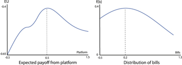

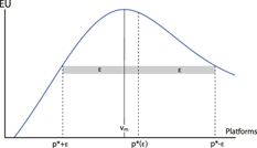


Comments
No Comments have been published for this article.