


1 Introduction
The long-term time evolution of linear flow on the flat unit torus has a well-established theory, giving rise to an important chapter in diophanine approximation. Here the continuous version of the classical Kronecker–Weyl equidistribution theorem can be formulated as follows; see [Reference Weyl12].
Theorem A. Suppose that
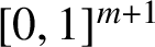
 $\mathbf {v}=(1,\gamma _{1},\ldots ,\gamma _{m})\in \mathbb {R}^{m+1}$
, where m is a positive integer and the real numbers
$\mathbf {v}=(1,\gamma _{1},\ldots ,\gamma _{m})\in \mathbb {R}^{m+1}$
, where m is a positive integer and the real numbers
 $1,\gamma _{1},\ldots ,\gamma _{m}$
are linearly independent over
$1,\gamma _{1},\ldots ,\gamma _{m}$
are linearly independent over
 $\mathbb {Q}$
. Then any half-infinite geodesic with direction given by
$\mathbb {Q}$
. Then any half-infinite geodesic with direction given by
 $\mathbf {v}$
is uniformly distributed on the unit torus
$\mathbf {v}$
is uniformly distributed on the unit torus
 $[0,1]^{m+1}$
.
$[0,1]^{m+1}$
.
We use the terms uniformly distributed and equidistributed with precisely the same meaning. Given any Jordan measurable test set
 $A\subseteq [0,1]^{m+1}$
, the proportion of time the half-infinite geodesic with direction
$A\subseteq [0,1]^{m+1}$
, the proportion of time the half-infinite geodesic with direction
 $\mathbf {v}$
falls into A is asymptotically equal to the
$\mathbf {v}$
falls into A is asymptotically equal to the
 $(m+1)$
-dimensional volume of A.
$(m+1)$
-dimensional volume of A.
Geodesic flow on the unit torus
 $[0,1]^{m+1}$
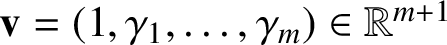
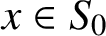
for positive integers m exhibits remarkable stability and predictability, giving rise to an integrable system. Here two particles moving on two parallel geodesics close to each other with the same speed and direction remain close forever. However, this is not the case when we consider nonintegrable systems. Figure 1 illustrates this point in the special case of the L-surface which clearly contains a singularity.
$[0,1]^{m+1}$
for positive integers m exhibits remarkable stability and predictability, giving rise to an integrable system. Here two particles moving on two parallel geodesics close to each other with the same speed and direction remain close forever. However, this is not the case when we consider nonintegrable systems. Figure 1 illustrates this point in the special case of the L-surface which clearly contains a singularity.

Figure 1 Geodesic flow on the L-surface.
One of the pioneering results concerning the equidistribution of geodesics on a large class of nonintegrable flat surfaces is due to Gutkin [Reference Gutkin4] and Veech [Reference Veech11] in the 1980s, and represents a first extension of the two-dimensional Kronecker–Weyl equidistribution theorem to a nonintegrable flat system such as a polysquare surface.
Before we proceed, let us define a polysquare region and a polysquare surface.
A polysquare region consists of a finite number of unit size squares such that (i) any two squares either are disjoint, or have a common edge, or have a common vertex; and (ii) there is edge-connectivity, that any two squares are joined by a chain of squares such that any two consecutive members of the chain share a common edge. Note that a polysquare region has a boundary.
To obtain a polysquare surface, or square tiled surface, we divide the collection of the horizontal boundary edges of the polysquare region into identified pairs, and divide the collection of the vertical boundary edges of the polysquare region into identified pairs. In this way, we obtain a closed surface equipped with a flat metric, so that it is a Riemann surface, with possible canonical singularities, where every square has zero curvature. We then refer to such a polysquare surface as a translation surface. Geodesic flow on a flat translation surface is one-direction linear flow.
The following result is often known as the Gutkin–Veech theorem.
Theorem B. A geodesic on any polysquare surface, with any starting point and any irrational slope, is equidistributed, unless it hits a singular point and becomes undefined.
Given the 70 years or so between the Kronecker–Weyl equidistribution theorem and the Gutkin–Veech theorem, it is clear that the singularities in nonintegrable systems lead to considerable difficulties. Meanwhile, a very natural question that arises from the Gutkin–Veech theorem concerns extensions of the Kronecker–Weyl equidistribution theorem to nonintegrable systems along similar lines but in higher dimensions. Observe that the Gutkin–Veech theorem is about two-dimensional nonintegrable flat systems. The methods there, unfortunately, do not seem to extend to the case of flat systems in higher dimensions. Indeed, as far as we are aware, there is no uniformity result in the literature concerning geodesics in
 $3$
-manifolds along these lines. The object of this paper is to study uniformity of half-infinite one-direction geodesics in polycube
$3$
-manifolds along these lines. The object of this paper is to study uniformity of half-infinite one-direction geodesics in polycube
 $3$
-manifolds and related questions.
$3$
-manifolds and related questions.
Before we proceed, let us define a polycube region and a polycube
 $3$
-manifold.
$3$
-manifold.
A polycube region consists of a finite number of unit size cubes such that (i) any two cubes either are disjoint, or have a common face, or have a common edge, or have a common vertex; and (ii) there is face-connectivity, that is any two cubes are joined by a chain of cubes such that any two consecutive members of the chain share a common face. Note that a polycube region has boundary.
To obtain a polycube
 $3$
-manifold, or cube tiled manifold, we divide the collection of the
$3$
-manifold, or cube tiled manifold, we divide the collection of the
 $xy$
-parallel faces of the polycube region into identified pairs, divide the collection of the
$xy$
-parallel faces of the polycube region into identified pairs, divide the collection of the
 $xz$
-parallel faces of the polycube region into identified pairs, and divide the collection of the
$xz$
-parallel faces of the polycube region into identified pairs, and divide the collection of the
 $yz$
-parallel faces of the polycube region into identified pairs. In this way, we obtain a closed
$yz$
-parallel faces of the polycube region into identified pairs. In this way, we obtain a closed
 $3$
-manifold equipped with a flat metric, with possible canonical singularities. We then refer to such a polycube
$3$
-manifold equipped with a flat metric, with possible canonical singularities. We then refer to such a polycube
 $3$
-manifold as a translation
$3$
-manifold as a translation
 $3$
-manifold. Geodesic flow in a flat translation
$3$
-manifold. Geodesic flow in a flat translation
 $3$
-manifold is one-direction linear flow.
$3$
-manifold is one-direction linear flow.
The known techniques seem to fall well short for establishing any comparable analog of the Gutkin–Veech theorem in this three-dimensional setting. Nevertheless, we can prove that for any given polycube
 $3$
-manifold
$3$
-manifold
 $\mathcal {P}$
, there are infinitely many special directions, which can be given explicitly, such that every half-infinite geodesic having such a direction is uniformly distributed in
$\mathcal {P}$
, there are infinitely many special directions, which can be given explicitly, such that every half-infinite geodesic having such a direction is uniformly distributed in
 $\mathcal {P}$
.
$\mathcal {P}$
.
A street, or a cyclic solid cylinder, in a polycube
 $3$
-manifold
$3$
-manifold
 $\mathcal {P}$
denotes a maximal cycle of consecutive unit cubes arranged in a linear fashion along one of the three coordinate directions. Thus, there are X-streets, Y-streets and Z-streets, where, for instance, a Z-street denotes a box of the form
$\mathcal {P}$
denotes a maximal cycle of consecutive unit cubes arranged in a linear fashion along one of the three coordinate directions. Thus, there are X-streets, Y-streets and Z-streets, where, for instance, a Z-street denotes a box of the form
 $$ \begin{align*} [a,a+1]\times[b,b+1]\times[c,c+\ell], \quad a,b,c,\ell\in\mathbb{Z}, \end{align*} $$
where the side of length
 $\ell \geqslant 1$
is parallel to the Z-axis. It is natural to call the integer
$\ell \geqslant 1$
is parallel to the Z-axis. It is natural to call the integer
 $\ell $
the length of the street. The street-LCM of
$\ell $
the length of the street. The street-LCM of
 $\mathcal {P}$
is the least common multiple of the lengths of the streets of
$\mathcal {P}$
is the least common multiple of the lengths of the streets of
 $\mathcal {P}$
.
$\mathcal {P}$
.
Using a new method, we can prove the following result.
Theorem 1.1. Suppose that
 $\mathcal {P}$
is an arbitrary polycube
$\mathcal {P}$
is an arbitrary polycube
 $3$
-manifold. Let
$3$
-manifold. Let
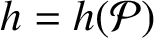 $h=h(\mathcal {P})$
denote the street-LCM of
$h=h(\mathcal {P})$
denote the street-LCM of
 $\mathcal {P}$
.
$\mathcal {P}$
.
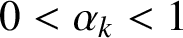
(i) Let
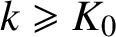
 $k\geqslant 1$
be any fixed integer, and let
$k\geqslant 1$
be any fixed integer, and let
 $\alpha _{k}$
be the root of the cubic equation
$\alpha _{k}$
be the root of the cubic equation
 $$ \begin{align} x^{3}+hkx-1=0, \quad \frac{1}{hk+1}<x<\frac{1}{hk}. \end{align} $$
Write
 $$ \begin{align} \mathbf{v}_{0}=(\alpha_{k},\alpha_{k}^{2},1), \quad \mathbf{v}_{1}=(1,\alpha_{k},\alpha_{k}^{2}), \quad \mathbf{v}_{2}=(\alpha_{k}^{2},1,\alpha_{k}). \end{align} $$
Then every half-infinite geodesic with direction given by
 $\mathbf {v}_{i}$
,
$\mathbf {v}_{i}$
,
 $i=0,1,2$
, is equidistributed in
$i=0,1,2$
, is equidistributed in
 $\mathcal {P}$
, provided that the integer parameter k is sufficiently large depending only on
$\mathcal {P}$
, provided that the integer parameter k is sufficiently large depending only on
 $\mathcal {P}$
. The test sets for uniformity are all three-dimensional Jordan measurable subsets of
$\mathcal {P}$
. The test sets for uniformity are all three-dimensional Jordan measurable subsets of
 $\mathcal {P}$
.
$\mathcal {P}$
.
(ii) Let A be an arbitrary three-dimensional Jordan measurable set in
 $\mathcal {P}$
, and let
$\mathcal {P}$
, and let
 $L(t)$
,
$L(t)$
,
 $0\leqslant t\leqslant T$
, be a finite geodesic with direction given by
$0\leqslant t\leqslant T$
, be a finite geodesic with direction given by
 $\mathbf {v}_{i}$
,
$\mathbf {v}_{i}$
,
 $i=0,1,2$
, in (1-1)–(1-2), with arc-length parametrization. Then there exist effectively computable explicit positive constants
$i=0,1,2$
, in (1-1)–(1-2), with arc-length parametrization. Then there exist effectively computable explicit positive constants
 $c_{1}=c_{1}(A;\alpha _{k})>0$
and
$c_{1}=c_{1}(A;\alpha _{k})>0$
and
 $c_{2}=c_{2}(A;\alpha _{k})>0$
such that
$c_{2}=c_{2}(A;\alpha _{k})>0$
such that
 $$ \begin{align*} \vert\{0\leqslant t\leqslant T:L(t)\in A\}\vert\geqslant c_1T, \end{align*} $$
provided that
 $T\geqslant c_{2}$
.
$T\geqslant c_{2}$
.
Part (i) is a time-qualitative result that does not say anything about the speed of convergence to uniformity. However, it is complemented by part (ii), which is a time-quantitative result exhibiting at least a weaker form of uniformity.
Theorem 1.1 only gives a small collection of slopes. Note that
 $1,\alpha _k,\alpha _k^2$
are linearly independent over
$1,\alpha _k,\alpha _k^2$
are linearly independent over
 $\mathbb {Q}$
, so Theorem 1.1 applied to the unit torus
$\mathbb {Q}$
, so Theorem 1.1 applied to the unit torus
 $[0,1]^3$
agrees with Theorem A. The majority of the remaining directions remain currently out of reach. We also do not know what happens beyond the class of polycube
$[0,1]^3$
agrees with Theorem A. The majority of the remaining directions remain currently out of reach. We also do not know what happens beyond the class of polycube
 $3$
-manifolds.
$3$
-manifolds.
We mention here that Theorems A, B and 1.1 have analogs on billiards in the unit cube, a polysquare region and a polycube region respectively, via a simple but very important discovery made more than
 $100$
years ago by König and Szücs [Reference König and Szücs6]. The underlying geometric trick is called unfolding. We illustrate the idea in the case of the unit square
$100$
years ago by König and Szücs [Reference König and Szücs6]. The underlying geometric trick is called unfolding. We illustrate the idea in the case of the unit square
 $[0,1]^{2}$
in Figure 2, where the
$[0,1]^{2}$
in Figure 2, where the
 $2\times 2$
torus in the picture on the right is a
$2\times 2$
torus in the picture on the right is a
 $4$
-fold covering of the unit square. Billiard flow in the square on the left is equivalent to geodesic flow in the torus on the right.
$4$
-fold covering of the unit square. Billiard flow in the square on the left is equivalent to geodesic flow in the torus on the right.

Figure 2 Unfolding a billiard orbit in the unit torus
 $[0,1]^{2}$
.
$[0,1]^{2}$
.
For further reading on the ergodic theory of flat surfaces, the reader is referred to the survey papers [Reference Hubert, Schmidt, Hasselblatt and Katok5, Reference Masur, Hasselblat and Katok8, Reference Masur, Tabachnikov, Hasselblat and Katok9, Reference Zorich, Cartier, Julia, Moussa and Vanhove13].
2 Geodesics in the L-solid manifold
We begin the proof of Theorem 1.1 with a discussion of the special case when the polycube
 $3$
-manifold in question is obtained as a translation
$3$
-manifold in question is obtained as a translation
 $3$
-manifold from the L-solid region shown in Figure 3. Here the three unit cubes of the region are called the top cube, the middle cube and the right cube. The street-LCM of the resulting L-solid
$3$
-manifold from the L-solid region shown in Figure 3. Here the three unit cubes of the region are called the top cube, the middle cube and the right cube. The street-LCM of the resulting L-solid
 $3$
-manifold is
$3$
-manifold is
 $2$
. We consider geodesics inside this manifold and, in particular, those with directions given by (1-1)–(1-2).
$2$
. We consider geodesics inside this manifold and, in particular, those with directions given by (1-1)–(1-2).

Figure 3 The L-solid region.
For convenience, we refer to the L-solid region or the L-solid
 $3$
-manifold simply as the L-solid.
$3$
-manifold simply as the L-solid.
We introduce a convenient labeling of the faces of the L-solid; see Figures 4 and 5.
The picture on the left in Figure 4 shows the three front faces of the L-solid, with
 $y=0$
. The front top square face
$y=0$
. The front top square face
 $Y_{3}$
has vertices
$Y_{3}$
has vertices
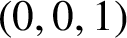 $(0,0,1)$
,
$(0,0,1)$
,
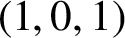 $(1,0,1)$
,
$(1,0,1)$
,
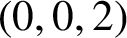 $(0,0,2)$
and
$(0,0,2)$
and
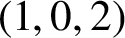 $(1,0,2)$
. We denote this fact by
$(1,0,2)$
. We denote this fact by
 $$ \begin{align*} Y_3=\operatorname{\mathrm{SQ}}\{(0,0,1),(1,0,1),(0,0,2),(1,0,2)\}. \end{align*} $$
The front middle and front right square faces are denoted respectively by
 $$ \begin{align*} Y_{1}&=\operatorname{\mathrm{SQ}}\{(0,0,0),(1,0,0),(0,0,1),(1,0,1)\},\\ Y_{2}&=\operatorname{\mathrm{SQ}}\{(1,0,0),(2,0,0),(1,0,1),(2,0,1)\}. \end{align*} $$
On the other hand, the picture on the right in Figure 4 shows the three back faces of the L-solid, with
 $y=1$
. The back top, back middle and back right square faces are denoted respectively by
$y=1$
. The back top, back middle and back right square faces are denoted respectively by
 $$ \begin{align*} Y_{6}&=\operatorname{\mathrm{SQ}}\{(0,1,1),(1,1,1),(0,1,2),(1,1,2)\},\\ Y_{4}&=\operatorname{\mathrm{SQ}}\{(0,1,0),(1,1,0),(0,1,1),(1,1,1)\},\\ Y_{5}&=\operatorname{\mathrm{SQ}}\{(1,1,0),(2,1,0),(1,1,1),(2,1,1)\}. \end{align*} $$
These six square faces are perpendicular to the y-axis, justifying use of the letter Y.
We see from Figure 5 that between the front and back faces, there are four faces
 $$ \begin{align*} X_{1}&=\operatorname{\mathrm{SQ}}\{(0,0,0),(0,1,0),(0,0,1),(0,1,1)\},\\ X_{2}&=\operatorname{\mathrm{SQ}}\{(0,0,1),(0,1,1),(0,0,2),(0,1,2)\},\\ X_{3}&=\operatorname{\mathrm{SQ}}\{(2,0,0),(2,1,0),(2,0,1),(2,1,1)\},\\ X_{4}&=\operatorname{\mathrm{SQ}}\{(1,0,1),(1,1,1),(1,0,2),(1,1,2)\}, \end{align*} $$
on the boundary of the L-solid that are perpendicular to the x-axis, another four faces
 $$ \begin{align*} Z_{1}&=\operatorname{\mathrm{SQ}}\{(0,0,0),(1,0,0),(0,1,0),(1,1,0)\},\\ Z_{2}&=\operatorname{\mathrm{SQ}}\{(1,0,0),(2,0,0),(1,1,0),(2,1,0)\},\\ Z_{3}&=\operatorname{\mathrm{SQ}}\{(0,0,2),(1,0,2),(0,1,2),(1,1,2)\},\\ Z_{4}&=\operatorname{\mathrm{SQ}}\{(1,0,1),(2,0,1),(1,1,1),(2,1,1)\}, \end{align*} $$
on the boundary of the L-solid that are perpendicular to the z-axis, and two inside faces
 $$ \begin{align*} X_{5}&=\operatorname{\mathrm{SQ}}\{(1,0,0),(1,1,0),(1,0,1),(1,1,1)\},\\ Z_{5}&=\operatorname{\mathrm{SQ}}\{(0,0,1),(1,0,1),(0,1,1),(1,1,1)\}. \end{align*} $$
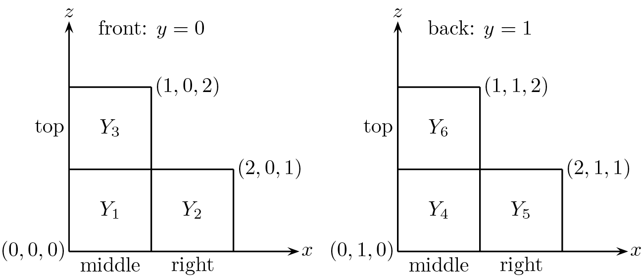
Figure 4 Labeling the front and back faces of the L-solid.

Figure 5 Labeling the rest of the faces of the L-solid.
Let
 $k\geqslant 1$
be an arbitrary but fixed integer. Assume that a segment of a geodesic
$k\geqslant 1$
be an arbitrary but fixed integer. Assume that a segment of a geodesic
 $\mathcal {L}_{k}$
starts from the origin
$\mathcal {L}_{k}$
starts from the origin
 $\mathbf {0}=(0,0,0)$
and ends at a point
$\mathbf {0}=(0,0,0)$
and ends at a point
 $C=(1,x,y)$
on the inside square face
$C=(1,x,y)$
on the inside square face
 $X_{5}$
, and in between hits the square face
$X_{5}$
, and in between hits the square face
 $Z_{3}$
on k separate occasions; see Figure 6, which shows the special case
$Z_{3}$
on k separate occasions; see Figure 6, which shows the special case
 $k=1$
.
$k=1$
.

Figure 6 First detour crossing in the L-solid:
 $k=1$
.
$k=1$
.
Let B denote the point on the square face
 $Z_{3}$
that
$Z_{3}$
that
 $\mathcal {L}_{k}$
hits on the last occasion before it bounces down to the point
$\mathcal {L}_{k}$
hits on the last occasion before it bounces down to the point
 $B^{\prime }$
and continues towards the point C.
$B^{\prime }$
and continues towards the point C.
Let A denote the point on the inside square face
 $Z_{5}$
that
$Z_{5}$
that
 $\mathcal {L}_{k}$
hits on the first occasion, and assume that
$\mathcal {L}_{k}$
hits on the first occasion, and assume that
 $A=(x,y,1)$
, so that its coordinates form a permutation of the coordinates of
$A=(x,y,1)$
, so that its coordinates form a permutation of the coordinates of
 $C=(1,x,y)$
with the same quantities x and y. It is easy to see that
$C=(1,x,y)$
with the same quantities x and y. It is easy to see that
 $B=(2kx,2ky,2)$
and
$B=(2kx,2ky,2)$
and
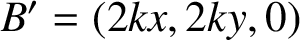 $B^{\prime }=(2kx,2ky,0)$
. The geometric fact that the two vectors
$B^{\prime }=(2kx,2ky,0)$
. The geometric fact that the two vectors
 $\mathbf {0} A$
and
$\mathbf {0} A$
and
 $B^{\prime }C$
are parallel gives rise to the equations
$B^{\prime }C$
are parallel gives rise to the equations
 $$ \begin{align*} \frac{1-2kx}{x}=\frac{x-2ky}{y}=\frac{y-0}{1}. \end{align*} $$
The first equality reduces to
 $y=x^{2}$
. Substituting this into the right-hand side and then equating with the left-hand side, we conclude that
$y=x^{2}$
. Substituting this into the right-hand side and then equating with the left-hand side, we conclude that
 $$ \begin{align} y=x^{2} \quad \mbox{and}\quad x^{3}+2kx-1=0. \end{align} $$
Note that the cubic polynomial
 $x^{3}+2kx-1$
is strictly increasing and has precisely one root
$x^{3}+2kx-1$
is strictly increasing and has precisely one root
 $\alpha _{k}$
satisfying
$\alpha _{k}$
satisfying
 $$ \begin{align} \frac{1}{2k+1}<\alpha_{k}<\frac{1}{2k}. \end{align} $$
Of course, (2-1)–(2-2) represent the special case of (1-1) when
 $h=2$
, the street-LCM of the L-solid.
$h=2$
, the street-LCM of the L-solid.
We now take
 $x=\alpha _{k}$
and
$x=\alpha _{k}$
and
 $y=\alpha ^{2}_{k}$
, and consider the segment of the geodesic
$y=\alpha ^{2}_{k}$
, and consider the segment of the geodesic
 $\mathcal {L}_{k}$
with direction given by
$\mathcal {L}_{k}$
with direction given by
 $\mathbf {v}_{0}=(\alpha _{k},\alpha ^{2}_{k},1)$
illustrated in Figure 6. Starting from the origin
$\mathbf {v}_{0}=(\alpha _{k},\alpha ^{2}_{k},1)$
illustrated in Figure 6. Starting from the origin
 $\mathbf {0}=(0,0,0)$
, this geodesic segment exhibits up-and-down zigzagging, and finally ends its journey at the point
$\mathbf {0}=(0,0,0)$
, this geodesic segment exhibits up-and-down zigzagging, and finally ends its journey at the point
 $C=(1,\alpha _{k},\alpha ^{2}_{k})$
on the middle square face
$C=(1,\alpha _{k},\alpha ^{2}_{k})$
on the middle square face
 $X_{5}$
. It represents a left-to-right detour crossing inside a tower-like three-dimensional street, where the latter is the union of the middle cube and the top cube. Observe that with
$X_{5}$
. It represents a left-to-right detour crossing inside a tower-like three-dimensional street, where the latter is the union of the middle cube and the top cube. Observe that with
 $0<\alpha _{k}<1$
, the geodesic
$0<\alpha _{k}<1$
, the geodesic
 $\mathcal {L}_{k}$
goes to the right faster than it goes to the back, and so crosses from one X-face to another faster than crossing from one Y-face to another.
$\mathcal {L}_{k}$
goes to the right faster than it goes to the back, and so crosses from one X-face to another faster than crossing from one Y-face to another.
The straight-line segment joining the two endpoints
 $\mathbf {0}$
and
$\mathbf {0}$
and
 $C=(1,\alpha _{k},\alpha ^{2}_{k})$
of this detour crossing is called the shortcut of this detour crossing.
$C=(1,\alpha _{k},\alpha ^{2}_{k})$
of this detour crossing is called the shortcut of this detour crossing.
The first extension of this particular zigzagging segment of the geodesic
 $\mathcal {L}_{k}$
with direction given by
$\mathcal {L}_{k}$
with direction given by
 $\mathbf {v}_{0}=(\alpha _{k},\alpha ^{2}_{k},1)$
starts from the point
$\mathbf {v}_{0}=(\alpha _{k},\alpha ^{2}_{k},1)$
starts from the point
 $C=(1,\alpha _{k},\alpha ^{2}_{k})$
on the square face
$C=(1,\alpha _{k},\alpha ^{2}_{k})$
on the square face
 $X_{5}$
and goes to the point
$X_{5}$
and goes to the point
 $D=(2,2\alpha _{k},2\alpha ^{2}_{k})$
on the right face
$D=(2,2\alpha _{k},2\alpha ^{2}_{k})$
on the right face
 $X_{3}$
; see Figure 7. This zigzagging extension hits the square face
$X_{3}$
; see Figure 7. This zigzagging extension hits the square face
 $Z_{4}$
on
$Z_{4}$
on
 $2k$
separate occasions, at the points
$2k$
separate occasions, at the points
 $(1+i\alpha _{k}-\alpha _{k}^{3},\alpha _{k}+i\alpha ^{2}_{k}-\alpha _{k}^{4},1)$
,
$(1+i\alpha _{k}-\alpha _{k}^{3},\alpha _{k}+i\alpha ^{2}_{k}-\alpha _{k}^{4},1)$
,
 $1\leqslant i\leqslant 2k$
, before ending at the point D on the square face
$1\leqslant i\leqslant 2k$
, before ending at the point D on the square face
 $X_{3}$
.
$X_{3}$
.

Figure 7 Second detour crossing in the L-solid:
 $k=1$
.
$k=1$
.
This zigzagging second segment of the geodesic
 $\mathcal {L}_{k}$
from C to D with direction given by
$\mathcal {L}_{k}$
from C to D with direction given by
 $\mathbf {v}_{0}$
represents a left-to-right detour crossing inside a three-dimensional street, which is simply the right cube. Again the straight-line segment joining the two endpoints C and D of this detour crossing is called the shortcut of this detour crossing.
$\mathbf {v}_{0}$
represents a left-to-right detour crossing inside a three-dimensional street, which is simply the right cube. Again the straight-line segment joining the two endpoints C and D of this detour crossing is called the shortcut of this detour crossing.
These two shortcuts
 $\mathbf {0} C$
and
$\mathbf {0} C$
and
 $CD$
, with endpoints
$CD$
, with endpoints
 $\mathbf {0}=(0,0,0)$
,
$\mathbf {0}=(0,0,0)$
,
 $C=(1,\alpha _{k},\alpha ^{2}_{k})$
and
$C=(1,\alpha _{k},\alpha ^{2}_{k})$
and
 $D=(2,2\alpha _{k},2\alpha ^{2}_{k})$
, are clearly collinear. In fact, the point C is the midpoint of the line segment
$D=(2,2\alpha _{k},2\alpha ^{2}_{k})$
, are clearly collinear. In fact, the point C is the midpoint of the line segment
 $\mathbf {0} D$
.
$\mathbf {0} D$
.
It is easy to see that this collinearity of the shortcuts is preserved as we continue and take the third, fourth and subsequent segments of the geodesic
 $\mathcal {L}_{k}$
starting from the origin with direction given by
$\mathcal {L}_{k}$
starting from the origin with direction given by
 $\mathbf {v}_{0}=(\alpha _{k},\alpha ^{2}_{k},1)$
. This collinearity means precisely that these consecutive shortcuts together form another geodesic
$\mathbf {v}_{0}=(\alpha _{k},\alpha ^{2}_{k},1)$
. This collinearity means precisely that these consecutive shortcuts together form another geodesic
 $\mathcal {L}^{*}_{k}$
starting from the origin, but it has a new direction given by
$\mathcal {L}^{*}_{k}$
starting from the origin, but it has a new direction given by
 $\mathbf {v}_{1}=(1,\alpha _{k},\alpha ^{2}_{k})$
obtained by a permutation of the coordinates of
$\mathbf {v}_{1}=(1,\alpha _{k},\alpha ^{2}_{k})$
obtained by a permutation of the coordinates of
 $\mathbf {v}_{0}$
. We refer to this new geodesic
$\mathbf {v}_{0}$
. We refer to this new geodesic
 $\mathcal {L}^{*}_{k}$
as the shortline of the original geodesic
$\mathcal {L}^{*}_{k}$
as the shortline of the original geodesic
 $\mathcal {L}_{k}$
. Formally,
$\mathcal {L}_{k}$
. Formally,
 $\mathbf {S}(\mathcal {L}_{k})=\mathcal {L}^{*}_{k}$
, where
$\mathbf {S}(\mathcal {L}_{k})=\mathcal {L}^{*}_{k}$
, where
 $\mathbf {S}$
denotes the shortline operation. In the special case
$\mathbf {S}$
denotes the shortline operation. In the special case
 $k=1$
, Figure 8 is basically Figures 6 and 7 put together. It shows the two parts of the zigzagging
$k=1$
, Figure 8 is basically Figures 6 and 7 put together. It shows the two parts of the zigzagging
 $\mathcal {L}_{k}$
from
$\mathcal {L}_{k}$
from
 $\mathbf {0}$
to D, with the point C separating the two parts. It also shows the corresponding shortline segment of
$\mathbf {0}$
to D, with the point C separating the two parts. It also shows the corresponding shortline segment of
 $\mathcal {L}^{*}_{k}$
, indicated by the dashed arrow, from
$\mathcal {L}^{*}_{k}$
, indicated by the dashed arrow, from
 $\mathbf {0}$
to D.
$\mathbf {0}$
to D.

Figure 8 Detour crossing and its shortline in the L-solid:
 $k=1$
.
$k=1$
.
The crucial fact is that the geodesic
 $\mathcal {L}_{k}$
and its shortline
$\mathcal {L}_{k}$
and its shortline
 $\mathcal {L}^{*}_{k}$
hit every square face
$\mathcal {L}^{*}_{k}$
hit every square face
 $X_{i}$
,
$X_{i}$
,
 $1\leqslant i\leqslant 5$
, at precisely the same points, like C and D in Figures 7 and 8. We refer to this observation as the X-face hitting property of the infinite geodesic
$1\leqslant i\leqslant 5$
, at precisely the same points, like C and D in Figures 7 and 8. We refer to this observation as the X-face hitting property of the infinite geodesic
 $\mathcal {L}_{k}$
and its shortline
$\mathcal {L}_{k}$
and its shortline
 $\mathcal {L}^{*}_{k}$
.
$\mathcal {L}^{*}_{k}$
.
The vector
 $\mathbf {v}_{1}=(1,\alpha _{k},\alpha ^{2}_{k})$
is clearly obtained from the vector
$\mathbf {v}_{1}=(1,\alpha _{k},\alpha ^{2}_{k})$
is clearly obtained from the vector
 $\mathbf {v}_{0}=(\alpha _{k},\alpha ^{2}_{k},1)$
by a left shift in the cyclic permutation of the coordinates
$\mathbf {v}_{0}=(\alpha _{k},\alpha ^{2}_{k},1)$
by a left shift in the cyclic permutation of the coordinates
 $$ \begin{align*} 1\to\alpha_{k}\to\alpha^{2}_{k}\to1. \end{align*} $$
Applying a second left shift in this cyclic permutation, we obtain in turn a new vector
 $\mathbf {v}_{2}=(\alpha ^{2}_{k},1,\alpha _{k})$
. It is easy to see that the shortline of the geodesic
$\mathbf {v}_{2}=(\alpha ^{2}_{k},1,\alpha _{k})$
. It is easy to see that the shortline of the geodesic
 $\mathcal {L}^{*}_{k}$
is a new geodesic
$\mathcal {L}^{*}_{k}$
is a new geodesic
 $\mathcal {L}^{**}_{k}$
that starts at the origin and has direction given by
$\mathcal {L}^{**}_{k}$
that starts at the origin and has direction given by
 $\mathbf {v}_{2}$
. Formally,
$\mathbf {v}_{2}$
. Formally,
 $\mathbf {S}(\mathcal {L}^{*}_{k})=\mathcal {L}^{**}_{k}$
. Note that
$\mathbf {S}(\mathcal {L}^{*}_{k})=\mathcal {L}^{**}_{k}$
. Note that
 $\mathcal {L}^{*}_{k}$
consists of front-to-back detour crossings, and
$\mathcal {L}^{*}_{k}$
consists of front-to-back detour crossings, and
 $\mathcal {L}^{**}_{k}$
is the union of the corresponding shortcuts. Observe that with
$\mathcal {L}^{**}_{k}$
is the union of the corresponding shortcuts. Observe that with
 $0<\alpha _{k}<1$
, the geodesic
$0<\alpha _{k}<1$
, the geodesic
 $\mathcal {L}^{*}_{k}$
goes to the back faster than it goes up, and so crosses from one Y-face to another faster than crossing from one Z-face to another.
$\mathcal {L}^{*}_{k}$
goes to the back faster than it goes up, and so crosses from one Y-face to another faster than crossing from one Z-face to another.
Again the crucial fact is that the geodesic
 $\mathcal {L}^{*}_{k}$
and its shortline
$\mathcal {L}^{*}_{k}$
and its shortline
 $\mathcal {L}^{**}_{k}$
hit every square face
$\mathcal {L}^{**}_{k}$
hit every square face
 $Y_{i}$
,
$Y_{i}$
,
 $1\leqslant i\leqslant 6$
, at precisely the same points. We refer to this observation as the Y-face hitting property of the infinite geodesic
$1\leqslant i\leqslant 6$
, at precisely the same points. We refer to this observation as the Y-face hitting property of the infinite geodesic
 $\mathcal {L}^{*}_{k}$
and its shortline
$\mathcal {L}^{*}_{k}$
and its shortline
 $\mathcal {L}^{**}_{k}$
.
$\mathcal {L}^{**}_{k}$
.
Applying a third left shift in the cyclic permutation, we return to the original direction given by
 $\mathbf {v}_{0}=(\alpha _{k},\alpha ^{2}_{k},1)$
. It is easy to see that the shortline of the geodesic
$\mathbf {v}_{0}=(\alpha _{k},\alpha ^{2}_{k},1)$
. It is easy to see that the shortline of the geodesic
 $\mathcal {L}^{**}_{k}$
is the original geodesic
$\mathcal {L}^{**}_{k}$
is the original geodesic
 $\mathcal {L}_{k}$
that starts at the origin and has direction vector
$\mathcal {L}_{k}$
that starts at the origin and has direction vector
 $\mathbf {v}_{0}$
. Formally,
$\mathbf {v}_{0}$
. Formally,
 $\mathbf {S}(\mathcal {L}^{**}_{k})=\mathcal {L}_{k}$
. Note that
$\mathbf {S}(\mathcal {L}^{**}_{k})=\mathcal {L}_{k}$
. Note that
 $\mathcal {L}^{**}_{k}$
consists of bottom to top detour crossings, and
$\mathcal {L}^{**}_{k}$
consists of bottom to top detour crossings, and
 $\mathcal {L}_{k}$
is the union of the corresponding shortcuts. Observe that with
$\mathcal {L}_{k}$
is the union of the corresponding shortcuts. Observe that with
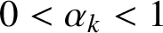 $0<\alpha _{k}<1$
, the geodesic
$0<\alpha _{k}<1$
, the geodesic
 $\mathcal {L}^{**}_{k}$
goes up faster than it goes to the right, and so crosses from one Z-face to another faster than crossing from one X-face to another.
$\mathcal {L}^{**}_{k}$
goes up faster than it goes to the right, and so crosses from one Z-face to another faster than crossing from one X-face to another.
Again the crucial fact is that the geodesic
 $\mathcal {L}^{**}_{k}$
and its shortline
$\mathcal {L}^{**}_{k}$
and its shortline
 $\mathcal {L}_{k}$
hit every square face
$\mathcal {L}_{k}$
hit every square face
 $Z_{i}$
,
$Z_{i}$
,
 $1\leqslant i\leqslant 5$
, at precisely the same points. We refer to this observation as the Z-face hitting property of the infinite geodesic
$1\leqslant i\leqslant 5$
, at precisely the same points. We refer to this observation as the Z-face hitting property of the infinite geodesic
 $\mathcal {L}^{**}_{k}$
and its shortline
$\mathcal {L}^{**}_{k}$
and its shortline
 $\mathcal {L}_{k}$
.
$\mathcal {L}_{k}$
.
The remarkable face hitting properties explain why we focus on geodesics with direction given by one of the vectors
 $$ \begin{align} \mathbf{v}_{0}=(\alpha_{k},\alpha^{2}_{k},1), \quad \mathbf{v}_{1}=(1,\alpha_{k},\alpha^{2}_{k}), \quad \mathbf{v}_{2}=(\alpha^{2}_{k},1,\alpha_{k}). \end{align} $$
We prove uniformity of such geodesics in the L-solid by applying an adaptation of an area magnification process via shortlines, developed in [Reference Beck, Chen and Yang1, Section 6.3]. To make the present paper self-contained, we explain this magnification process in full detail in Sections 3 and 4.
In [Reference Beck, Chen and Yang1, Section 6.3], we establish time-quantitative density. In fact, we establish a nearly optimal form of density of such geodesics in the L-solid. To explain this, let
 $\eta>0$
be an arbitrarily small but fixed positive number. We say that a half-infinite geodesic
$\eta>0$
be an arbitrarily small but fixed positive number. We say that a half-infinite geodesic
 $\mathcal {L}$
in the L-solid is
$\mathcal {L}$
in the L-solid is
 $\eta $
-nearly superdense if there exists an effectively computable explicit threshold
$\eta $
-nearly superdense if there exists an effectively computable explicit threshold
 $N_{0}(\eta )$
such that, for every integer
$N_{0}(\eta )$
such that, for every integer
 $n\geqslant N_{0}(\eta )$
, the initial segment of
$n\geqslant N_{0}(\eta )$
, the initial segment of
 $\mathcal {L}$
with length
$\mathcal {L}$
with length
 $n^{2+\eta }$
intersects every axis-parallel cube of side length
$n^{2+\eta }$
intersects every axis-parallel cube of side length
 $1/n$
in the L-solid.
$1/n$
in the L-solid.
Remark 2.1. The optimal property would be to replace
 $n^{2+\eta }$
by a constant multiple of
$n^{2+\eta }$
by a constant multiple of
 $n^{2}$
. We call this superdensity. Unfortunately we are not able to establish superdensity in the three-dimensional case.
$n^{2}$
. We call this superdensity. Unfortunately we are not able to establish superdensity in the three-dimensional case.
The following result is [Reference Beck, Chen and Yang1, Theorem 6.1.2].
Time-quantitative density A. Let
 $\eta>0$
be fixed. There exists a threshold
$\eta>0$
be fixed. There exists a threshold
 $K_{0}(\eta )$
such that for every integer
$K_{0}(\eta )$
such that for every integer
 $k\geqslant K_{0}(\eta )$
, any half-infinite geodesic in the L-solid with direction given by one of the vectors in (2-3), where
$k\geqslant K_{0}(\eta )$
, any half-infinite geodesic in the L-solid with direction given by one of the vectors in (2-3), where
 $\alpha _{k}$
is a root of the cubic equation
$\alpha _{k}$
is a root of the cubic equation
 $x^{3}+2kx-1=0$
satisfying (2-2), is
$x^{3}+2kx-1=0$
satisfying (2-2), is
 $\eta $
-nearly superdense in the L-solid.
$\eta $
-nearly superdense in the L-solid.
In fact, we need only a straightforward corollary of the above result, obtained by choosing any fixed value of
 $\eta $
in the interval
$\eta $
in the interval
 $0<\eta <1$
.
$0<\eta <1$
.
Time-quantitative density B. Let
 $k\geqslant K_{0}$
, where
$k\geqslant K_{0}$
, where
 $K_{0}$
is an effectively computable sufficiently large absolute constant. Let
$K_{0}$
is an effectively computable sufficiently large absolute constant. Let
 $\kappa>0$
be arbitrarily small but fixed. Then there exists an explicit threshold
$\kappa>0$
be arbitrarily small but fixed. Then there exists an explicit threshold
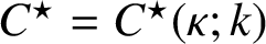 $C^{\star} = C^{\star }(\kappa ;k)$
such that every geodesic segment in the L-solid with length
$C^{\star} = C^{\star }(\kappa ;k)$
such that every geodesic segment in the L-solid with length
 $C^{\star }$
and direction given by one of the vectors in (2-3), where
$C^{\star }$
and direction given by one of the vectors in (2-3), where
 $\alpha _{k}$
is a root of the cubic equation
$\alpha _{k}$
is a root of the cubic equation
 $x^{3}+2kx-1=0$
satisfying (2-2), intersects every square of side length
$x^{3}+2kx-1=0$
satisfying (2-2), intersects every square of side length
 $\kappa $
on the surface of the L-solid.
$\kappa $
on the surface of the L-solid.
Our first goal is to establish uniformity of these special geodesics in the L-solid. Unfortunately, our proof does not give any error term, so what we can prove here is time-qualitative uniformity. The proof consists of four major steps:
(i) preparation for the magnification process;
(ii) the magnification process;
(iii) grids and iteration; and
(vi) conclusion via time-quantitative density B.
We cover these in the next four sections.
3 Preparation for the magnification process
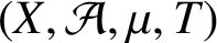
We use Birkhoff’s well-known pointwise ergodic theorem concerning measure-preserving systems
 $(X,\mathcal {A},\mu ,T)$
. The triple
$(X,\mathcal {A},\mu ,T)$
. The triple
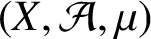 $(X,\mathcal {A},\mu )$
is a measure space, where X is the underlying space,
$(X,\mathcal {A},\mu )$
is a measure space, where X is the underlying space,
 $\mathcal {A}$
is a
$\mathcal {A}$
is a
 $\sigma $
-algebra of sets in X, while
$\sigma $
-algebra of sets in X, while
 $\mu $
is a nonnegative
$\mu $
is a nonnegative
 $\sigma $
-additive measure on X with
$\sigma $
-additive measure on X with
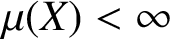 $\mu (X)<\infty $
, and
$\mu (X)<\infty $
, and
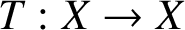 $T:X\to X$
is a measure-preserving transformation, so that
$T:X\to X$
is a measure-preserving transformation, so that
 $T^{-1}A\in \mathcal {A}$
and
$T^{-1}A\in \mathcal {A}$
and
 $\mu (T^{-1}A)=\mu (A)$
for every
$\mu (T^{-1}A)=\mu (A)$
for every
 $A\in \mathcal {A}$
. Here we simply apply ergodic theory, and do not expect the reader to have any serious expertise in the subject. Knowledge of Lebesgue integral and basic measure theory suffices.
$A\in \mathcal {A}$
. Here we simply apply ergodic theory, and do not expect the reader to have any serious expertise in the subject. Knowledge of Lebesgue integral and basic measure theory suffices.
Let
 $L^{1}(X,\mathcal {A},\mu )$
denote the space of measurable and integrable functions in the measure space
$L^{1}(X,\mathcal {A},\mu )$
denote the space of measurable and integrable functions in the measure space
 $(X,\mathcal {A},\mu )$
. Then Birkhoff’s pointwise ergodic theorem says that for every function
$(X,\mathcal {A},\mu )$
. Then Birkhoff’s pointwise ergodic theorem says that for every function
 $f\in L^{1}(X,\mathcal {A},\mu )$
, the limit
$f\in L^{1}(X,\mathcal {A},\mu )$
, the limit
 $$ \begin{align} \lim_{m\to\infty}\frac{1}{m}\sum_{j=0}^{m-1}f(T^{j}x)=f^{*}(x) \end{align} $$
exists for
 $\mu $
-almost every
$\mu $
-almost every
 $x\in X$
, where
$x\in X$
, where
 $f^{*}\in L^{1}(X,\mathcal {A},\mu )$
is a T-invariant measurable function satisfying the condition
$f^{*}\in L^{1}(X,\mathcal {A},\mu )$
is a T-invariant measurable function satisfying the condition
 $$ \begin{align*} \int_{X}f\,{d}\mu=\int_{X}f^{*}\,{d}\mu. \end{align*} $$
A particularly important special case is when T is ergodic, when every measurable T-invariant set
 $A\in \mathcal {A}$
is trivial in the precise sense that
$A\in \mathcal {A}$
is trivial in the precise sense that
 $\mu (A)=0$
or
$\mu (A)=0$
or
 $\mu (A)=\mu (X)$
. This is equivalent to the assertion that every measurable T-invariant function is constant
$\mu (A)=\mu (X)$
. This is equivalent to the assertion that every measurable T-invariant function is constant
 $\mu $
-almost everywhere.
$\mu $
-almost everywhere.
If T is ergodic, then (3-1) simplifies to
 $$ \begin{align} \lim_{m\to\infty}\frac{1}{m}\sum_{j=0}^{m-1}f(T^{j}x)=\int_{X}f\,{d}\mu, \end{align} $$
and the right-hand side of (3-1) is the same constant for
 $\mu $
-almost every
$\mu $
-almost every
 $x\in X$
.
$x\in X$
.
The remarkable intuitive interpretation of (3-2) is that the time average on the left-hand side is equal to the space average on the right-hand side.
Unfortunately, Birkhoff’s theorem does not give the speed of convergence in (3-1) or (3-2).
Next we explain how ergodicity and Birkhoff’s theorem are used in the proof. Recall the labeling of the square faces of the L-solid shown in Figures 4 and 5. Consider the five square faces
 $X_{i}$
,
$X_{i}$
,
 $1\leqslant i\leqslant 5$
, each with area
$1\leqslant i\leqslant 5$
, each with area
 $1$
. Boundary identification in the L-solid gives
$1$
. Boundary identification in the L-solid gives
 $X_{1}=X_{3}$
and
$X_{1}=X_{3}$
and
 $X_{2}=X_{4}$
, so that we simply have the three square faces
$X_{2}=X_{4}$
, so that we simply have the three square faces
 $X_{1},X_{2},X_{5}$
. We define our underlying measure space as the set
$X_{1},X_{2},X_{5}$
. We define our underlying measure space as the set
 $X_{0}=X_{1}\cup X_{2}\cup X_{5}$
with the usual area, or two-dimensional Lebesgue measure, denoted by
$X_{0}=X_{1}\cup X_{2}\cup X_{5}$
with the usual area, or two-dimensional Lebesgue measure, denoted by
![]() . Then
. Then
 $X_{0}$
is in fact a compact flat surface, that is, a polysquare surface, of area
$X_{0}$
is in fact a compact flat surface, that is, a polysquare surface, of area
 $3$
, so that
$3$
, so that
![]() .
.
We use the special direction
 $\mathbf {v}_{1}=(1,\alpha _{k},\alpha ^{2}_{k})$
, where
$\mathbf {v}_{1}=(1,\alpha _{k},\alpha ^{2}_{k})$
, where
 $\alpha _{k}$
is a root of the cubic equation
$\alpha _{k}$
is a root of the cubic equation
 $x^{3}+2kx-1=0$
satisfying (2-2).
$x^{3}+2kx-1=0$
satisfying (2-2).
The
 $\mathbf {v}_{1}$
-flow in the L-solid defines a
$\mathbf {v}_{1}$
-flow in the L-solid defines a
![]() -preserving transformation on
-preserving transformation on
 $X_{0}$
in the natural way as illustrated in Figure 9. For instance, the point
$X_{0}$
in the natural way as illustrated in Figure 9. For instance, the point
 $C\in X_{5}$
is mapped to the point
$C\in X_{5}$
is mapped to the point
 $D\in X_{3}=X_{1}$
via the
$D\in X_{3}=X_{1}$
via the
 $\mathbf {v}_{1}$
-flow. Similarly, the
$\mathbf {v}_{1}$
-flow. Similarly, the
 $\mathbf {v}_{1}$
-flow maps almost every point of the measure-space
$\mathbf {v}_{1}$
-flow maps almost every point of the measure-space
 $X_{0}$
to another point of
$X_{0}$
to another point of
 $X_{0}$
; here we ignore the singularities. Let
$X_{0}$
; here we ignore the singularities. Let
 $T=T_{\mathbf {v}_{1}}:X_{0}\to X_{0}$
denote this
$T=T_{\mathbf {v}_{1}}:X_{0}\to X_{0}$
denote this
![]() -preserving transformation. In particular,
-preserving transformation. In particular,
 $T(C)=D$
in Figure 9.
$T(C)=D$
in Figure 9.

Figure 9 Transformation
 $T=T_{\mathbf {v}_{1}}$
, where
$T=T_{\mathbf {v}_{1}}$
, where
 $\mathbf {v}_{1}=CD$
.
$\mathbf {v}_{1}=CD$
.
The major part of our argument is to prove that this particular transformation
 $T=T_{\mathbf {v}_{1}}$
is ergodic. In other words, we need to show that if
$T=T_{\mathbf {v}_{1}}$
is ergodic. In other words, we need to show that if
 $S\subset X_{0}$
is a measurable T-invariant set, then
$S\subset X_{0}$
is a measurable T-invariant set, then
![]() or
or
![]() . Once ergodicity is established, it is relatively straightforward to derive uniformity via Birkhoff’s theorem, at least for almost every starting point.
. Once ergodicity is established, it is relatively straightforward to derive uniformity via Birkhoff’s theorem, at least for almost every starting point.
We prove ergodicity by contradiction. Assume to the contrary that there is a nontrivial measurable T-invariant set
 $S_{0}\subset X_{0}$
such that
$S_{0}\subset X_{0}$
such that
![]() . We then derive a contradiction by using a version of the magnification process via shortlines developed in [Reference Beck, Chen and Yang1, Sections 6.2–6.3]. Note that our assumption ensures that the complement
. We then derive a contradiction by using a version of the magnification process via shortlines developed in [Reference Beck, Chen and Yang1, Sections 6.2–6.3]. Note that our assumption ensures that the complement
 $S_{0}^{c}=X_{0}\setminus S_{0}$
is another nontrivial measurable T-invariant set.
$S_{0}^{c}=X_{0}\setminus S_{0}$
is another nontrivial measurable T-invariant set.
Removing a set of measure zero, we can clearly assume that for every point
 $x\in S_{0}$
,
$x\in S_{0}$
,
 $T^{j}x$
is well defined for every
$T^{j}x$
is well defined for every
 $j\geqslant 1$
.
$j\geqslant 1$
.
Given a point
 $z\in X_{0}$
and a radius
$z\in X_{0}$
and a radius
 $0<r<1/2$
, let
$0<r<1/2$
, let
 $D(z;r)$
denote the circular disk of radius r and centered at z. Then
$D(z;r)$
denote the circular disk of radius r and centered at z. Then
 $D(z;r)$
has area
$D(z;r)$
has area
 $r^{2}\pi $
. Note that
$r^{2}\pi $
. Note that
 $D(z;r)\subset X_{0}$
, due to the fact that
$D(z;r)\subset X_{0}$
, due to the fact that
 $X_{0}$
is a compact flat surface. Lebesgue’s density theorem then says that, for almost every
$X_{0}$
is a compact flat surface. Lebesgue’s density theorem then says that, for almost every
 $z\in S_{0}$
,
$z\in S_{0}$
,

and for almost every
 $z\in S_{0}^{c}=X_{0}\setminus S_{0}$
,
$z\in S_{0}^{c}=X_{0}\setminus S_{0}$
,

Let
 $n\geqslant 1$
be an integer, and divide each of the square faces
$n\geqslant 1$
be an integer, and divide each of the square faces
 $X_{1},X_{2},X_{5}$
into
$X_{1},X_{2},X_{5}$
into
 $n^{2}$
congruent squares of area
$n^{2}$
congruent squares of area
 $n^{-2}$
in the standard way. We refer to them as small n-squares. Thus, we have
$n^{-2}$
in the standard way. We refer to them as small n-squares. Thus, we have
 $3n^{2}$
small n-squares in
$3n^{2}$
small n-squares in
 $X_{0}$
.
$X_{0}$
.
Lemma 3.1. Suppose that the real number
 $\tau $
satisfies
$\tau $
satisfies
Let
 $\varepsilon>0$
be arbitrarily small but fixed. Then there exists a finite integer-valued threshold
$\varepsilon>0$
be arbitrarily small but fixed. Then there exists a finite integer-valued threshold
 $n=n(S_{0};\varepsilon )$
such that there exist at least
$n=n(S_{0};\varepsilon )$
such that there exist at least
 $(\tau -\varepsilon )n^{2}$
small n-squares Q with
$(\tau -\varepsilon )n^{2}$
small n-squares Q with

Proof. Since
 $S_{0}^{c}=X_{0}\setminus S_{0}$
is Lebesgue measurable, given any
$S_{0}^{c}=X_{0}\setminus S_{0}$
is Lebesgue measurable, given any
 $\delta>0$
, there exist finitely many disjoint axis-parallel rectangles such that their union V is
$\delta>0$
, there exist finitely many disjoint axis-parallel rectangles such that their union V is
 $\delta $
-close to
$\delta $
-close to
 $S_{0}^{c}=X_{0}\setminus S_{0}$
in the sense of the measure of the symmetric difference, so that
$S_{0}^{c}=X_{0}\setminus S_{0}$
in the sense of the measure of the symmetric difference, so that
It follows that
Since V is a finite union of disjoint axis-parallel rectangles, there clearly exists an integer-valued threshold
 $n=n(V;\delta )$
such that the union
$n=n(V;\delta )$
such that the union
 $V_{1}$
of the small n-squares Q contained in V has measure at least
$V_{1}$
of the small n-squares Q contained in V has measure at least
Let
 $\mathcal {B}$
denote the set of n-squares Q that do not satisfy (3-4), so that
$\mathcal {B}$
denote the set of n-squares Q that do not satisfy (3-4), so that

Then

so that
 $$ \begin{align*} \vert\mathcal{B}\vert\leqslant\frac{\delta n^2}{\varepsilon}=\frac{\varepsilon n^2}{3}, \end{align*} $$
if we take
 $\delta =\varepsilon ^{2}/3$
. We may assume without loss of generality that
$\delta =\varepsilon ^{2}/3$
. We may assume without loss of generality that
 $0<\varepsilon <1$
. Deleting the n-squares
$0<\varepsilon <1$
. Deleting the n-squares
 $Q\in \mathcal {B}$
, we see that
$Q\in \mathcal {B}$
, we see that
 $V_{1}$
contains at least
$V_{1}$
contains at least
 $$ \begin{align*} (\tau-2\delta)n^2-\frac{\varepsilon n^2}{3}=\bigg(\tau-\frac{2\varepsilon^2}{3}-\frac{\varepsilon}{3}\bigg)n^2>(\tau-\varepsilon)n^2 \end{align*} $$
n-squares Q that satisfy (3-4). Finally, note that V and
 $\delta $
depend on
$\delta $
depend on
 $S_{0}$
and
$S_{0}$
and
 $\varepsilon $
.
$\varepsilon $
.
We now continue our discussion under the assumptions of Lemma 3.1.
Let
 $\mathcal {Q}$
denote the set of small n-squares Q that satisfy the bound (3-4). For notational convenience, we may write
$\mathcal {Q}$
denote the set of small n-squares Q that satisfy the bound (3-4). For notational convenience, we may write
 $$ \begin{align} \mathcal{Q}=\{Q_{i}:i\in I\}. \end{align} $$
Then, in view of Lemma 3.1, we have
 $$ \begin{align} \vert I\vert=\vert\mathcal{Q}\vert\geqslant(\tau -\varepsilon)n^{2}. \end{align} $$
For every
 $i\in I$
in (3-5), let
$i\in I$
in (3-5), let
 $\chi _{i}$
denote the characteristic function of the subset
$\chi _{i}$
denote the characteristic function of the subset
 $S_{0}\cap Q_{i}$
of
$S_{0}\cap Q_{i}$
of
 $X_{0}$
, so that
$X_{0}$
, so that
 $$ \begin{align*} \chi_i(x)=\begin{cases} 1\quad&\mbox{if }x\in S_{0}\cap Q_{i},\\ 0\quad&\mbox{otherwise}. \end{cases} \end{align*} $$
Applying Birkhoff’s theorem in the form (3-1) to each function
 $\chi _{i}$
,
$\chi _{i}$
,
 $i\in I$
, we have
$i\in I$
, we have
 $$ \begin{align} \lim_{m\to\infty}\frac{1}{m}\sum_{j=0}^{m-1}\chi_{i}(T^{j}x)=\chi^{*}_{i}(x), \end{align} $$
for
 $\mu $
-almost every
$\mu $
-almost every
 $x\in X_{0}$
, where each
$x\in X_{0}$
, where each
 $\chi ^{*}_{i}(x)$
is some T-invariant measurable function satisfying the condition
$\chi ^{*}_{i}(x)$
is some T-invariant measurable function satisfying the condition

Combining (3-4) and (3-8), for every
 $i\in I$
, we have
$i\in I$
, we have

Using the left-hand side of (3-7), we deduce that
 $\chi ^{*}_{i}(x)$
is nonnegative
$\chi ^{*}_{i}(x)$
is nonnegative
 $\mu $
-almost everywhere. It then follows from (3-9) that
$\mu $
-almost everywhere. It then follows from (3-9) that

Taking the minimum of the function
 $$ \begin{align*} g(x)=\frac{1}{\vert I\vert}\sum_{i\in I}\chi^*_i(x) \end{align*} $$
over
 $x\in S_{0}$
, or getting arbitrarily close to that, (3-10) implies the existence of some
$x\in S_{0}$
, or getting arbitrarily close to that, (3-10) implies the existence of some
 $x_{0}\in S_{0}$
such that
$x_{0}\in S_{0}$
such that
 $$ \begin{align} 0\leqslant\frac{1}{\vert I\vert}\sum_{i\in I}\chi^{*}_{i}(x_{0})<\frac{\varepsilon}{(3-\tau)n^{2}}, \end{align} $$
where the factor
 $3-\tau $
in the denominator on the right-hand side is the measure of
$3-\tau $
in the denominator on the right-hand side is the measure of
 $S_{0}$
given by (3-3).
$S_{0}$
given by (3-3).
It now follows from (3-11) that there exists a subset
 $I_{0}\subset I$
satisfying
$I_{0}\subset I$
satisfying
 $\vert I_{0}\vert \geqslant \vert I\vert /2$
such that
$\vert I_{0}\vert \geqslant \vert I\vert /2$
such that
 $$ \begin{align} 0\leqslant\chi^{*}_{i}(x_{0})\leqslant\frac{2\varepsilon}{(3-\tau)n^{2}} \quad\mbox{for every }i\in I_{0}. \end{align} $$
Note that in view of (3-6), we have
 $$ \begin{align} \vert I_{0}\vert\geqslant\frac{(\tau-\varepsilon)n^{2}}{2}. \end{align} $$
On the other hand, combining (3-7) and (3-12), we see that
 $$ \begin{align} \lim_{m\to\infty}\frac{1}{m}\sum_{j=0}^{m-1}\chi_{i}(T^{j}x_{0}) =\chi^{*}_{i}(x_{0}) \leqslant\frac{2\varepsilon}{(3-\tau)n^{2}} \quad\mbox{for every }i\in I_{0}. \end{align} $$
Since every point in
 $S_{0}$
is nonpathological,
$S_{0}$
is nonpathological,
 $T^{j}x_{0}$
is well defined for every
$T^{j}x_{0}$
is well defined for every
 $j\geqslant 1$
. It also follows from (3-14) that there exists a finite threshold
$j\geqslant 1$
. It also follows from (3-14) that there exists a finite threshold
 $m_{0}$
such that for every integer
$m_{0}$
such that for every integer
 $m\geqslant m_{0}$
,
$m\geqslant m_{0}$
,
 $$ \begin{align} \frac{1}{m}\sum_{j=0}^{m-1}\chi_{i}(T^{j}x_{0}) <\frac{3\varepsilon}{(3-\tau)n^{2}} \quad\mbox{for every }i\in I_{0}. \end{align} $$
We recall that
 $\chi _{i}$
is the characteristic function of the set
$\chi _{i}$
is the characteristic function of the set
 $S_{0}\cap Q_{i}$
. Since
$S_{0}\cap Q_{i}$
. Since
 $x_{0}$
is in the nontrivial T-invariant set
$x_{0}$
is in the nontrivial T-invariant set
 $S_{0}$
, the infinite sequence
$S_{0}$
, the infinite sequence
 $T^{j}x_{0}$
,
$T^{j}x_{0}$
,
 $j\geqslant 0$
, never enters the set
$j\geqslant 0$
, never enters the set
 $Q_{i}\setminus S_{0}$
. Let
$Q_{i}\setminus S_{0}$
. Let
 $\chi ^{\star \star }_{i}$
denote the characteristic function of the small n-square
$\chi ^{\star \star }_{i}$
denote the characteristic function of the small n-square
 $Q_{i}$
, so that
$Q_{i}$
, so that
 $$ \begin{align*} \chi^{\star\star}_i(x)=\begin{cases} 1\quad&\mbox{if }x\in Q_{i},\\ 0\quad&\mbox{otherwise}. \end{cases} \end{align*} $$
Then (3-15) is equivalent to the assertion that for every integer
 $m\geqslant m_{0}$
,
$m\geqslant m_{0}$
,
 $$ \begin{align} \frac{1}{m}\sum_{j=0}^{m-1}\chi^{\star\star}_{i}(T^{j}x_{0}) <\frac{3\varepsilon}{(3-\tau)n^{2}} \quad\mbox{for every }i\in I_{0}. \end{align} $$
Note that every small n-square
 $Q_{i}$
has area
$Q_{i}$
has area
 $n^{-2}$
. Then (3-16) implies that for every integer
$n^{-2}$
. Then (3-16) implies that for every integer
 $m\geqslant m_{0}$
,
$m\geqslant m_{0}$
,

Choosing a sufficiently small
 $\varepsilon>0$
, this gives the message that the small n-square
$\varepsilon>0$
, this gives the message that the small n-square
 $Q_{i}$
is grossly undervisited by the sequence
$Q_{i}$
is grossly undervisited by the sequence
 $T^{j}x_{0}$
,
$T^{j}x_{0}$
,
 $0\leqslant j\leqslant m-1$
.
$0\leqslant j\leqslant m-1$
.
Indeed, since
![]() , the term
, the term

represents the expected value of the number of the points
 $T^{j}x_{0}\in Q_{i}$
,
$T^{j}x_{0}\in Q_{i}$
,
 $0\leqslant j\leqslant m-1$
. If
$0\leqslant j\leqslant m-1$
. If
 $0<\tau <3$
is fixed and
$0<\tau <3$
is fixed and
 $\varepsilon>0$
is sufficiently small, then the factor
$\varepsilon>0$
is sufficiently small, then the factor
 $$ \begin{align*} \frac{9\varepsilon}{3-\tau} \end{align*} $$
in (3-17) justifies the term grossly undervisited. Here we assume that the expected value (3-18) is large, which is clearly possible, since
 $m\geqslant m_{0}$
can be arbitrarily large.
$m\geqslant m_{0}$
can be arbitrarily large.
Note that every
 $Q_{i}$
, where
$Q_{i}$
, where
 $i\in I_{0}$
, is grossly undervisited. In view of (3-13), these represent a positive proportion of the total number
$i\in I_{0}$
, is grossly undervisited. In view of (3-13), these represent a positive proportion of the total number
 $3n^{2}$
of small n-squares in
$3n^{2}$
of small n-squares in
 $X_{0}$
.
$X_{0}$
.
Suppose that every small n-square
 $Q_{i}$
,
$Q_{i}$
,
 $i\in I_{0}$
, is divided into
$i\in I_{0}$
, is divided into
 $$ \begin{align} \frac{6\varepsilon m}{(3-\tau)n^{2}} \end{align} $$
convex parts with equal area; for notational simplicity, let us assume here that the quantity (3-19) is an integer. We refer to these as the tiny convex parts. Since
 $$ \begin{align*} \frac{6\varepsilon m}{(3-\tau)n^2}=2\frac{9\varepsilon}{(3-\tau)}\frac{m}{3n^2}, \end{align*} $$
it follows from (3-17) and (3-19) that at least half of these tiny convex parts of
 $Q_{i}$
are empty, that is, they do not contain any element of the sequence
$Q_{i}$
are empty, that is, they do not contain any element of the sequence
 $T^{j}x_{0}$
,
$T^{j}x_{0}$
,
 $0\leqslant j\leqslant m-1$
. We refer to them as the empty tiny convex parts of
$0\leqslant j\leqslant m-1$
. We refer to them as the empty tiny convex parts of
 $Q_{i}$
,
$Q_{i}$
,
 $i\in I_{0}$
.
$i\in I_{0}$
.
In the next section, we give an explicit construction of these tiny convex parts of
 $Q_{i}$
,
$Q_{i}$
,
 $i\in I_{0}$
, which have the same area.
$i\in I_{0}$
, which have the same area.
4 The magnification process
We consider iterated area magnification of convex sets on the faces by using the three X–Y–Z-face hitting properties and the
 $3$
-periodicity of the shortline process. We elaborate on this.
$3$
-periodicity of the shortline process. We elaborate on this.
Figure 10 illustrates area magnification via tilted parallel projection.

Figure 10 Magnifying the area via tilted parallel projection.
In order to visualize the parallel projection a little better, we have included an extra copy of three unit square faces, indicated by the dashed line squares, on the plane
 $y=1$
in cartesian
$y=1$
in cartesian
 $3$
-space that can be identified with the square faces
$3$
-space that can be identified with the square faces
 $Y_{4},Y_{5},Y_{6}$
of the L-solid. We start with a parallelogram
$Y_{4},Y_{5},Y_{6}$
of the L-solid. We start with a parallelogram
 $S_{0}=ABCD$
on the square face
$S_{0}=ABCD$
on the square face
 $X_{3}$
. Using the
$X_{3}$
. Using the
 $\mathbf {v}_{1}$
-flow indicated by the arrow, where
$\mathbf {v}_{1}$
-flow indicated by the arrow, where
 $\mathbf {v}_{1}=(1,\alpha _{k},\alpha ^{2}_{k})$
is the direction vector of the shortline
$\mathbf {v}_{1}=(1,\alpha _{k},\alpha ^{2}_{k})$
is the direction vector of the shortline
 $\mathcal {L}^{*}_{k}$
of the geodesic
$\mathcal {L}^{*}_{k}$
of the geodesic
 $\mathcal {L}_{k}$
, we project the parallelogram on to the plane
$\mathcal {L}_{k}$
, we project the parallelogram on to the plane
 $y=1$
. For simplicity, suppose that it is projected on to unit squares identified with
$y=1$
. For simplicity, suppose that it is projected on to unit squares identified with
 $Y_{4}\cup Y_{5}$
, as shown. This tilted parallel projection maps the parallelogram
$Y_{4}\cup Y_{5}$
, as shown. This tilted parallel projection maps the parallelogram
 $S_{0}$
to a new parallelogram
$S_{0}$
to a new parallelogram
 $S_{1}=A^{\prime }B^{\prime }C^{\prime }D^{\prime }$
, and the area of
$S_{1}=A^{\prime }B^{\prime }C^{\prime }D^{\prime }$
, and the area of
 $S_{1}$
is
$S_{1}$
is
 $1/\alpha _{k}$
times the area of
$1/\alpha _{k}$
times the area of
 $S_{0}$
. We say that in Figure 10, the image of
$S_{0}$
. We say that in Figure 10, the image of
 $S_{0}=ABCD$
splits, in the sense that the image parallelogram
$S_{0}=ABCD$
splits, in the sense that the image parallelogram
 $S_{1}=A^{\prime }B^{\prime }C^{\prime }D^{\prime }$
is located on more than one square face. We aim to avoid splitting as much as possible.
$S_{1}=A^{\prime }B^{\prime }C^{\prime }D^{\prime }$
is located on more than one square face. We aim to avoid splitting as much as possible.
But we do not stop here. We want to describe a full
 $3$
-cycle
$3$
-cycle
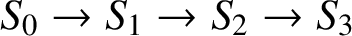 $S_{0}\to S_{1}\to S_{2}\to S_{3}$
as illustrated in Figure 11, where
$S_{0}\to S_{1}\to S_{2}\to S_{3}$
as illustrated in Figure 11, where
 $S_{2}$
is on a Z-face and
$S_{2}$
is on a Z-face and
 $S_{3}$
returns to an X-face.
$S_{3}$
returns to an X-face.

Figure 11 Illustrating the
 $3$
-cycle of the magnification process.
$3$
-cycle of the magnification process.
In general, we start with a parallelogram
 $S_{0}$
on some square face
$S_{0}$
on some square face
 $X_{i}$
of the L-solid that is contained in a plane
$X_{i}$
of the L-solid that is contained in a plane
 $x=x_{0}^{*}$
in cartesian
$x=x_{0}^{*}$
in cartesian
 $3$
-space, where
$3$
-space, where
 $x_{0}^{*}$
is an integer.
$x_{0}^{*}$
is an integer.
As a first step, let us project
 $S_{0}$
by the vector
$S_{0}$
by the vector
 $\mathbf {v}_{1}=(1,\alpha _{k},\alpha _{k}^{2})$
to a parallelogram
$\mathbf {v}_{1}=(1,\alpha _{k},\alpha _{k}^{2})$
to a parallelogram
 $S_{1}$
on a plane
$S_{1}$
on a plane
 $y=y_{1}^{*}$
, where
$y=y_{1}^{*}$
, where
 $y_{1}^{*}$
is an integer, with the point
$y_{1}^{*}$
is an integer, with the point
 $(x_{0}^{*},c_{1},c_{2})\in S_{0}$
at the center projected to the point
$(x_{0}^{*},c_{1},c_{2})\in S_{0}$
at the center projected to the point
 $(c_{3},y_{1}^{*},c_{4})\in S_{1}$
. If
$(c_{3},y_{1}^{*},c_{4})\in S_{1}$
. If
 $\mathbf {v}_{1}=(1,\alpha _{k},\alpha _{k}^{2})$
projects a point
$\mathbf {v}_{1}=(1,\alpha _{k},\alpha _{k}^{2})$
projects a point
 $(x_{0}^{*},c_{1}+y_{0},c_{2}+z_{0})\in S_{0}$
to the point
$(x_{0}^{*},c_{1}+y_{0},c_{2}+z_{0})\in S_{0}$
to the point
 $(c_{3}+x_{1},y_{1}^{*},c_{4}+z_{1})\in S_{1}$
, then a simple calculation shows that
$(c_{3}+x_{1},y_{1}^{*},c_{4}+z_{1})\in S_{1}$
, then a simple calculation shows that
 $$ \begin{align*} x_1=-\frac{y_0}{\alpha_k}=\frac{z_1-z_0}{\alpha_k^2}. \end{align*} $$
Hence,
 $x_{1}=-\alpha _{k}^{-1}y_{0}$
and
$x_{1}=-\alpha _{k}^{-1}y_{0}$
and
 $z_{1}=z_{0}-\alpha _{k}y_{0}$
, and so
$z_{1}=z_{0}-\alpha _{k}y_{0}$
, and so
 $$ \begin{align} \begin{pmatrix} x_{1}\\ z_{1} \end{pmatrix} =\begin{pmatrix} -\alpha_{k}^{-1}&0\\ -\alpha_{k}&1 \end{pmatrix} \begin{pmatrix} y_{0}\\ z_{0} \end{pmatrix}. \end{align} $$
As a second step, let us project
 $S_{1}$
by the vector
$S_{1}$
by the vector
 $\mathbf {v}_{2}=(\alpha _{k}^{2},1,\alpha _{k})$
to a parallelogram
$\mathbf {v}_{2}=(\alpha _{k}^{2},1,\alpha _{k})$
to a parallelogram
 $S_{2}$
on a plane
$S_{2}$
on a plane
 $z=z_{2}^{*}$
, where
$z=z_{2}^{*}$
, where
 $z_{2}^{*}$
is an integer, with the point
$z_{2}^{*}$
is an integer, with the point
 $(c_{3},y_{1}^{*},c_{4})\in S_{1}$
at the center projected to the point
$(c_{3},y_{1}^{*},c_{4})\in S_{1}$
at the center projected to the point
 $(c_{5},c_{6},z_{2}^{*})\in S_{2}$
. If
$(c_{5},c_{6},z_{2}^{*})\in S_{2}$
. If
 $\mathbf {v}_{2}=(\alpha _{k}^{2},1,\alpha _{k})$
projects a point
$\mathbf {v}_{2}=(\alpha _{k}^{2},1,\alpha _{k})$
projects a point
 $(c_{3}+x_{1},y_{1}^{*},c_{4}+z_{1})\in S_{1}$
to the point
$(c_{3}+x_{1},y_{1}^{*},c_{4}+z_{1})\in S_{1}$
to the point
 $(c_{5}+x_{2},c_{6}+y_{2},z_{2}^{*})\in S_{2}$
, then a simple calculation shows that
$(c_{5}+x_{2},c_{6}+y_{2},z_{2}^{*})\in S_{2}$
, then a simple calculation shows that
 $$ \begin{align*} \frac{x_2-x_1}{\alpha_k^2}=y_2=-\frac{z_1}{\alpha_k}. \end{align*} $$
Hence,
 $x_{2}=x_{1}-\alpha _{k} z_{1}$
and
$x_{2}=x_{1}-\alpha _{k} z_{1}$
and
 $y_{2}=-\alpha _{k}^{-1}z_{1}$
, and so
$y_{2}=-\alpha _{k}^{-1}z_{1}$
, and so
 $$ \begin{align} \begin{pmatrix} x_{2}\\ y_{2} \end{pmatrix} =\begin{pmatrix} 1&-\alpha_{k}\\ 0&-\alpha_{k}^{-1} \end{pmatrix} \begin{pmatrix} x_{1}\\ z_{1} \end{pmatrix}. \end{align} $$
As a final step, let us project
 $S_{2}$
by the vector
$S_{2}$
by the vector
 $\mathbf {v}_{0}=(\alpha _{k},\alpha _{k}^{2},1)$
to a parallelogram
$\mathbf {v}_{0}=(\alpha _{k},\alpha _{k}^{2},1)$
to a parallelogram
 $S_{3}$
on a plane
$S_{3}$
on a plane
 $x=x_{3}^{*}$
, where
$x=x_{3}^{*}$
, where
 $x_{3}^{*}$
is an integer, with the point
$x_{3}^{*}$
is an integer, with the point
 $(c_{5},c_{6},z_{2}^{*})\in S_{2}$
at the center projected to the point
$(c_{5},c_{6},z_{2}^{*})\in S_{2}$
at the center projected to the point
 $(x_{3}^{*},c_{7},c_{8})\in S_{3}$
. If
$(x_{3}^{*},c_{7},c_{8})\in S_{3}$
. If
 $\mathbf {v}_{0}=(\alpha _{k},\alpha _{k}^{2},1)$
projects a point
$\mathbf {v}_{0}=(\alpha _{k},\alpha _{k}^{2},1)$
projects a point
 $(c_{5}+x_{2},c_{6}+y_{2},z_{2}^{*})\in S_{2}$
to the point
$(c_{5}+x_{2},c_{6}+y_{2},z_{2}^{*})\in S_{2}$
to the point
 $(x_{3}^{*},c_{7}+y_{3},c_{8}+z_{3})\in S_{3}$
, then simple calculation shows that
$(x_{3}^{*},c_{7}+y_{3},c_{8}+z_{3})\in S_{3}$
, then simple calculation shows that
 $$ \begin{align*} -\frac{x_2}{\alpha_k}=\frac{y_3-y_2}{\alpha_k^2}=z_3. \end{align*} $$
Hence,
 $y_{3}=y_{2}-\alpha _{k} x_{2}$
and
$y_{3}=y_{2}-\alpha _{k} x_{2}$
and
 $z_{3}=-\alpha _{k}^{-1}x_{2}$
, and so
$z_{3}=-\alpha _{k}^{-1}x_{2}$
, and so
 $$ \begin{align} \begin{pmatrix} y_{3}\\ z_{3} \end{pmatrix} =\begin{pmatrix} -\alpha_{k}&1\\ -\alpha_{k}^{-1}&0 \end{pmatrix} \begin{pmatrix} x_{2}\\ y_{2} \end{pmatrix}. \end{align} $$
Combining (4-1)–(4-3), we see that this three-step magnification process has resulted in the transition
 $$ \begin{align*} \begin{pmatrix} y_3\\ z_3 \end{pmatrix} =\begin{pmatrix} -\alpha_k&1\\ -\alpha_k^{-1}&0 \end{pmatrix} \begin{pmatrix} 1&-\alpha_k\\ 0&-\alpha_k^{-1} \end{pmatrix} \begin{pmatrix} -\alpha_k^{-1}&0\\ -\alpha_k&1 \end{pmatrix} \begin{pmatrix} y\\ z \end{pmatrix}. \end{align*} $$
The transition matrix in question is
 $$ \begin{align*} \mathcal{A}=\begin{pmatrix} -\alpha_k&1\\ -\alpha_k^{-1}&0 \end{pmatrix} \begin{pmatrix} 1&-\alpha_k\\ 0&-\alpha_k^{-1} \end{pmatrix} \begin{pmatrix} -\alpha_k^{-1}&0\\ -\alpha_k&1 \end{pmatrix} =\begin{pmatrix} 2-\alpha_k^3&\alpha_k^2-\alpha_k^{-1}\\ \alpha_k^{-2}-\alpha_k&1 \end{pmatrix}. \end{align*} $$
The eigenvalues of this matrix are the roots of the quadratic equation
 $$ \begin{align*} \det\begin{pmatrix} 2-\alpha_k^3-\Lambda&\alpha_k^2-\alpha_k^{-1}\\ \alpha_k^{-2}-\alpha_k&1-\Lambda \end{pmatrix} =0, \end{align*} $$
or
 $\Lambda ^{2}-(3-\alpha _{k}^{3})\Lambda +\alpha _{k}^{-3}=0$
, with solutions
$\Lambda ^{2}-(3-\alpha _{k}^{3})\Lambda +\alpha _{k}^{-3}=0$
, with solutions
 $$ \begin{align} \Lambda_{i}=\frac{(3-\alpha_{k}^{3})\pm\mathrm{i}\sqrt{4\alpha_{k}^{-3}-(3-\alpha_{k}^{3})^{2}}}{2}, \quad i=1,2, \end{align} $$
and corresponding eigenvectors
 $$ \begin{align} \mathbf{W}_{i}=\bigg(\frac{\Lambda_{i}-1}{\alpha_{k}^{-2}-\alpha_{k}},1\bigg), \quad i=1,2. \end{align} $$
Note that the two eigenvalues are complex conjugates of each other, as are the first coordinates of the two eigenvectors. It follows that the two vectors
 $$ \begin{align} \mathbf{u}_{1}=\mathbf{W}_{1}+\mathbf{W}_{2} \quad\mbox{and}\quad \mathbf{u}_{2}=\frac{1}{\mathrm{i}}(\mathbf{W}_{1}-\mathbf{W}_{2}) \end{align} $$
have real coordinates. Indeed,
 $\mathbf {u}_{1}=(u_{1,1},u_{1,2})$
, where
$\mathbf {u}_{1}=(u_{1,1},u_{1,2})$
, where
 $$ \begin{align} u_{1,1}=\frac{2-\alpha_{k}^{3}}{\alpha_{k}^{-2}-\alpha_{k}} \quad\mbox{and}\quad u_{1,2}=2, \end{align} $$
and
 $\mathbf {u}_{2}=(u_{2,1},u_{2,2})$
, where
$\mathbf {u}_{2}=(u_{2,1},u_{2,2})$
, where
 $$ \begin{align} u_{2,1}=\frac{\sqrt{4\alpha_{k}^{-3}-(3-\alpha_{k}^{3})^{2}}}{\alpha_{k}^{-2}-\alpha_{k}} \quad\mbox{and}\quad u_{2,2}=0, \end{align} $$
if we ensure that
 $u_{2,1}$
is positive.
$u_{2,1}$
is positive.
These precise formulas motivate us to start the area magnification process with a small parallelogram
 $S_{0}$
on an X-face that lies on a plane
$S_{0}$
on an X-face that lies on a plane
 $x=x_{0}^{*}$
in cartesian
$x=x_{0}^{*}$
in cartesian
 $3$
-space, and with some very special properties attached to it. Omitting reference to the x-coordinate, we ensure that the nonparallel sides of
$3$
-space, and with some very special properties attached to it. Omitting reference to the x-coordinate, we ensure that the nonparallel sides of
 $S_{0}$
are parallel to
$S_{0}$
are parallel to
 $\mathbf {u}_{1}$
and
$\mathbf {u}_{1}$
and
 $\mathbf {u}_{2}$
, with lengths, respectively,
$\mathbf {u}_{2}$
, with lengths, respectively,
 $$ \begin{align} \delta\vert\mathbf{u}_{1}\vert=\delta(u_{1,1}^{2}+u_{1,2}^{2})^{1/2} \quad\mbox{and}\quad \delta\vert\mathbf{u}_{2}\vert=\delta u_{2,1}, \end{align} $$
where
 $\delta>0$
is a small fixed real number.
$\delta>0$
is a small fixed real number.
The three-step magnification process transforms
 $S_{0}$
into a parallelogram
$S_{0}$
into a parallelogram
 $S_{3}$
with the nonparallel sides parallel to the vector
$S_{3}$
with the nonparallel sides parallel to the vector
 $$ \begin{align*} \mathbf{u}_1^{(1)} =\mathcal{A}\mathbf{u}_1 =\mathcal{A}(\mathbf{W}_1+\mathbf{W}_2) =\mathcal{A}\mathbf{W}_1+\mathcal{A}\mathbf{W}_2 =\Lambda_1\mathbf{W}_1+\Lambda_2\mathbf{W}_2, \end{align*} $$
with real coordinates and of length
 $$ \begin{align*} \delta\vert\Lambda_1\mathbf{W}_1+\Lambda_2\mathbf{W}_2\vert, \end{align*} $$
and parallel to the vector
 $$ \begin{align*} \mathbf{u}_2^{(1)} =\mathcal{A}\mathbf{u}_2 =\frac{1}{\mathrm{i}}\mathcal{A}(\mathbf{W}_1-\mathbf{W}_2)r =\frac{1}{\mathrm{i}}(\mathcal{A}\mathbf{W}_1-\mathcal{A}\mathbf{W}_2) =\frac{1}{\mathrm{i}}(\Lambda_1\mathbf{W}_1-\Lambda_2\mathbf{W}_2), \end{align*} $$
with real coordinates and of length
 $$ \begin{align*} \delta\vert\Lambda_1\mathbf{W}_1-\Lambda_2\mathbf{W}_2\vert. \end{align*} $$
Indeed, this three-step magnification process repeated
 $r\geqslant 1$
times transforms
$r\geqslant 1$
times transforms
 $S_{0}$
into a parallelogram
$S_{0}$
into a parallelogram
 $S_{3r}$
on some X-face with the nonparallel sides parallel to the vector
$S_{3r}$
on some X-face with the nonparallel sides parallel to the vector
 $$ \begin{align} \mathbf{u}_{1}^{(r)} =\Lambda_{1}^{r}\mathbf{W}_{1}+\Lambda_{2}^{r}\mathbf{W}_{2}, \end{align} $$
with real coordinates and of length
 $$ \begin{align} \delta\vert\Lambda_{1}^{r}\mathbf{W}_{1}+\Lambda_{2}^{r}\mathbf{W}_{2}\vert, \end{align} $$
and parallel to the vector
 $$ \begin{align} \mathbf{u}_{2}^{(r)} =\frac{1}{\mathrm{i}}(\Lambda_{1}^{r}\mathbf{W}_{1}-\Lambda_{2}^{r}\mathbf{W}_{2}), \end{align} $$
with real coordinates and of length
 $$ \begin{align} \delta\vert\Lambda_{1}^{r}\mathbf{W}_{1}-\Lambda_{2}^{r}\mathbf{W}_{2}\vert. \end{align} $$
We clearly wish to understand how far the parallelogram
 $S_{3r}$
differs from the original parallelogram
$S_{3r}$
differs from the original parallelogram
 $S_{0}$
. In particular, we wish to show that it does not look like a long needle, with one side substantially longer than the other.
$S_{0}$
. In particular, we wish to show that it does not look like a long needle, with one side substantially longer than the other.
Assume that k is a fixed large integer.
First we estimate the area of
 $S_{3r}$
. It is clear, since
$S_{3r}$
. It is clear, since
 $u_{2,2}=0$
, that
$u_{2,2}=0$
, that
 $$ \begin{align} \operatorname{\mathrm{area}}(S_{0}) =\delta^{2}\vert u_{1,2}\vert\vert u_{2,1}\vert =(4+o_{k}(1))\delta^{2}\alpha_{k}^{1/2}. \end{align} $$
It then follows from the magnification process that
 $$ \begin{align} \operatorname{\mathrm{area}}(S_{3r}) =\alpha_{k}^{-3r}\operatorname{\mathrm{area}}(S_{0}) =(4+o_{k}(1))\delta^{2}\alpha_{k}^{-3r}\alpha_{k}^{1/2}. \end{align} $$
Next, we estimate the maximum side length of
 $S_{3r}$
. Note first of all that it clearly follows from (4-4) that
$S_{3r}$
. Note first of all that it clearly follows from (4-4) that
 $$ \begin{align*} \vert\Lambda_i\vert=\alpha_k^{-3/2}, \quad i=1,2. \end{align*} $$
Combining this with (4-5), we see that
 $$ \begin{align*} \vert\mathbf{W}_i\vert\leqslant2, \quad i=1,2. \end{align*} $$
It follows, on noting that the side lengths of
 $S_{3r}$
are given by (4-11) and (4-13), that the maximum side length of
$S_{3r}$
are given by (4-11) and (4-13), that the maximum side length of
 $S_{3r}$
satisfies
$S_{3r}$
satisfies
 $$ \begin{align} \operatorname{\mathrm{max-sidelength}}(S_{3r}) \leqslant\delta(\vert\Lambda_{1}\vert^{r}\vert\mathbf{W}_{1}\vert+\vert\Lambda_{2}\vert^{r}\vert\mathbf{W}_{2}\vert) \leqslant4\delta\alpha_{k}^{-3r/2}. \end{align} $$
Combining (4-15) and (4-16), we deduce that
 $$ \begin{align} \frac{(\operatorname{\mathrm{max-sidelength}}(S_{3r}))^{2}}{\operatorname{\mathrm{area}}(S_{3r})}\leqslant\frac{4+o_{k}(1)}{\alpha_{k}^{1/2}}. \end{align} $$
This shows that uniformly
 $S_{3r}$
does not look like a long needle.
$S_{3r}$
does not look like a long needle.
Recall that towards the end of the previous section, we wish to divide each small n-square
 $Q_{i}$
,
$Q_{i}$
,
 $i\in I_{0}$
, into
$i\in I_{0}$
, into
 $$ \begin{align} \frac{6\varepsilon m}{(3-\tau)n^{2}} \end{align} $$
convex parts with equal area, referred to as the tiny convex parts, and that for notational simplicity, we assume that the quantity (4-18) is an integer. Recall also that at least half of these tiny convex parts of
 $Q_{i}$
do not contain any element of the sequence
$Q_{i}$
do not contain any element of the sequence
 $T^{j}x_{0}$
,
$T^{j}x_{0}$
,
 $0\leqslant j\leqslant m-1$
, and that we refer to them as the empty tiny convex parts of
$0\leqslant j\leqslant m-1$
, and that we refer to them as the empty tiny convex parts of
 $Q_{i}$
,
$Q_{i}$
,
 $i\in I_{0}$
. We are now ready to give the explicit construction.
$i\in I_{0}$
. We are now ready to give the explicit construction.
Since every empty tiny convex part of
 $Q_{i}$
,
$Q_{i}$
,
 $i\in I_{0}$
, has relatively large area, we can employ the area magnification process on any of them. Of course the magnified image of an empty set is also empty. We show that there exists at least one such empty tiny convex part of some
$i\in I_{0}$
, has relatively large area, we can employ the area magnification process on any of them. Of course the magnified image of an empty set is also empty. We show that there exists at least one such empty tiny convex part of some
 $Q_{i}$
,
$Q_{i}$
,
 $i\in I_{0}$
, which avoids image-splitting during the entire area magnification process.
$i\in I_{0}$
, which avoids image-splitting during the entire area magnification process.
We define the tiny convex parts as congruent parallelograms on an X-face such that one side is parallel to
 $\mathbf {u}_{1}$
with length
$\mathbf {u}_{1}$
with length
 $\delta \vert \mathbf {u}_{1}\vert $
, and the other side is parallel to
$\delta \vert \mathbf {u}_{1}\vert $
, and the other side is parallel to
 $\mathbf {u}_{2}$
with length
$\mathbf {u}_{2}$
with length
 $\delta \vert \mathbf {u}_{2}\vert $
; see (4-5)–(4-9). Thus, we consider a parallelogram lattice
$\delta \vert \mathbf {u}_{2}\vert $
; see (4-5)–(4-9). Thus, we consider a parallelogram lattice
 $$ \begin{align} \Omega=\Omega(\mathbf{u}_{1},\mathbf{u}_{2};\delta) \end{align} $$
on the plane, where any fundamental parallelogram
 $\mathcal {P}\in \Omega $
, an atom of
$\mathcal {P}\in \Omega $
, an atom of
 $\Omega $
, has sides
$\Omega $
, has sides
 $\delta \mathbf {u}_{1}$
and
$\delta \mathbf {u}_{1}$
and
 $\delta \mathbf {u}_{2}$
. The concrete value of the parameter
$\delta \mathbf {u}_{2}$
. The concrete value of the parameter
 $\delta>0$
will be specified later.
$\delta>0$
will be specified later.
It is a minor irritation that the parallelogram lattice
 $\Omega $
in (4-19) may not tile a unit size square precisely. However, we show later that, with an appropriate choice of the parameters, this technical issue has a totally negligible effect.
$\Omega $
in (4-19) may not tile a unit size square precisely. However, we show later that, with an appropriate choice of the parameters, this technical issue has a totally negligible effect.
The whole magnification process consists of a large number of consecutive
 $3$
-cycles. It makes the calculations more convenient if we write the total number of consecutive
$3$
-cycles. It makes the calculations more convenient if we write the total number of consecutive
 $3$
-cycles as
$3$
-cycles as
 $\ell -O(1)$
, where the value of the constant
$\ell -O(1)$
, where the value of the constant
 $O(1)$
will be specified later.
$O(1)$
will be specified later.
We choose the parameters
 $\delta $
and
$\delta $
and
 $\ell $
such that
$\ell $
such that
 $$ \begin{align} \delta\vert\Lambda^{\ell}_{1}\vert=\delta\vert\Lambda^{\ell}_{2}\vert =\delta\alpha_{k}^{-3\ell/2}\asymp1. \end{align} $$
This will be made more precise later.
The area of any fundamental parallelogram in the lattice
 $\Omega =\Omega (\mathbf {u}_{1},\mathbf {u}_{2};\delta )$
defined in (4-19) is chosen to be precisely equal to
$\Omega =\Omega (\mathbf {u}_{1},\mathbf {u}_{2};\delta )$
defined in (4-19) is chosen to be precisely equal to
 $(3-\tau )/6\varepsilon m$
. Combining this with (4-14), the area of any fundamental parallelogram in the lattice
$(3-\tau )/6\varepsilon m$
. Combining this with (4-14), the area of any fundamental parallelogram in the lattice
 $\Omega =\Omega (\mathbf {u}_{1},\mathbf {u}_{2};\delta )$
is equal to
$\Omega =\Omega (\mathbf {u}_{1},\mathbf {u}_{2};\delta )$
is equal to
 $$ \begin{align} (4+o_{k}(1))\delta^{2}\alpha_{k}^{1/2}=\frac{3-\tau}{6\varepsilon m}. \end{align} $$
Since the area of an arbitrary small n-square
 $Q_{i}$
,
$Q_{i}$
,
 $i\in I_{0}$
, is equal to
$i\in I_{0}$
, is equal to
 $n^{-2}$
, it follows that the number of the fundamental parallelograms
$n^{-2}$
, it follows that the number of the fundamental parallelograms
 $\mathcal {P}$
in
$\mathcal {P}$
in
 $\Omega =\Omega (\mathbf {u}_{1},\mathbf {u}_{2};\delta )$
that intersect
$\Omega =\Omega (\mathbf {u}_{1},\mathbf {u}_{2};\delta )$
that intersect
 $Q_{i}$
is between
$Q_{i}$
is between
 $5\varepsilon m/(3-\tau )n^{2}$
and
$5\varepsilon m/(3-\tau )n^{2}$
and
 $7\varepsilon m/(3-\tau )n^{2}$
, where the number would be precisely
$7\varepsilon m/(3-\tau )n^{2}$
, where the number would be precisely
 $6\varepsilon m/(3-\tau )n^{2}$
in the case of perfect tiling, assuming that m is sufficiently large.
$6\varepsilon m/(3-\tau )n^{2}$
in the case of perfect tiling, assuming that m is sufficiently large.
We now take the fundamental parallelograms
 $\mathcal {P}$
of
$\mathcal {P}$
of
 $\Omega =\Omega (\mathbf {u}_{1},\mathbf {u}_{2};\delta )$
in
$\Omega =\Omega (\mathbf {u}_{1},\mathbf {u}_{2};\delta )$
in
 $Q_{i}$
as the tiny convex parts mentioned above. Then it follows that there are at least
$Q_{i}$
as the tiny convex parts mentioned above. Then it follows that there are at least
 $$ \begin{align*} \frac{5\varepsilon m}{(3-\tau)n^2}=\frac{5}{3}\frac{9\varepsilon}{(3-\tau)}\frac{m}{3n^2} \end{align*} $$
fundamental parallelograms in
 $Q_{i}$
. It then follows from (3-17) that a proportion of at least
$Q_{i}$
. It then follows from (3-17) that a proportion of at least
 $1-(3/5)=2/5$
of the fundamental parallelograms
$1-(3/5)=2/5$
of the fundamental parallelograms
 $\mathcal {P}$
in
$\mathcal {P}$
in
 $Q_{i}$
are empty, that is, they do not contain any element of the sequence
$Q_{i}$
are empty, that is, they do not contain any element of the sequence
 $T^{j}x_{0}$
,
$T^{j}x_{0}$
,
 $0\leqslant j\leqslant m-1$
. We refer to them as the empty fundamental parallelograms
$0\leqslant j\leqslant m-1$
. We refer to them as the empty fundamental parallelograms
 $\mathcal {P}$
in
$\mathcal {P}$
in
 $Q_{i}$
,
$Q_{i}$
,
 $i\in I_{0}$
. There are at least
$i\in I_{0}$
. There are at least
 $$ \begin{align*} \frac{2\varepsilon m}{(3-\tau)n^2} \end{align*} $$
of them. Combining this with (3-13), there are at least
 $$ \begin{align} \frac{(\tau-\varepsilon)n^{2}}{2}\frac{2\varepsilon m}{(3-\tau)n^{2}}=\frac{\varepsilon(\tau-\varepsilon)m}{3-\tau} \end{align} $$
empty fundamental parallelograms
 $\mathcal {P}$
in
$\mathcal {P}$
in
 $X_{0}$
.
$X_{0}$
.
Since
![]() , noting that the area of a fundamental parallelogram is given by (4-21), there are
, noting that the area of a fundamental parallelogram is given by (4-21), there are
 $$ \begin{align} \frac{3}{(3-\tau)/{6\varepsilon m}}\pm\varepsilon^{2}m=\bigg(\frac{18\varepsilon}{3-\tau}\pm\varepsilon^{2}\bigg)m \end{align} $$
fundamental parallelograms of the lattice
 $\Omega =\Omega (\mathbf {u}_{1},\mathbf {u}_{2};\delta )$
in
$\Omega =\Omega (\mathbf {u}_{1},\mathbf {u}_{2};\delta )$
in
 $X_{0}$
, assuming m is large enough. Here, the error term
$X_{0}$
, assuming m is large enough. Here, the error term
 $\pm \varepsilon ^{2}m$
comes from the contribution near the border.
$\pm \varepsilon ^{2}m$
comes from the contribution near the border.
Comparing (4-22) and (4-23), we conclude that the ratio of empty fundamental parallelograms
 $\mathcal {P}$
in
$\mathcal {P}$
in
 $X_{0}$
compared to the total number in
$X_{0}$
compared to the total number in
 $X_{0}$
is at least
$X_{0}$
is at least
 $$ \begin{align} \frac{\tau-\varepsilon}{20}, \end{align} $$
assuming that
 $\varepsilon>0$
is sufficiently small.
$\varepsilon>0$
is sufficiently small.
Our basic idea is that each such grossly undervisited small n-square
 $Q_{i}$
has many pairwise disjoint convex empty sets
$Q_{i}$
has many pairwise disjoint convex empty sets
 $\mathcal {P}\in \Omega =\Omega (\mathbf {u}_{1},\mathbf {u}_{2};\delta )$
with the same nonnegligible area, for which we can apply the area magnification process via shortlines. In the magnification process, we work with the concrete half-infinite geodesic that starts from the special point
$\mathcal {P}\in \Omega =\Omega (\mathbf {u}_{1},\mathbf {u}_{2};\delta )$
with the same nonnegligible area, for which we can apply the area magnification process via shortlines. In the magnification process, we work with the concrete half-infinite geodesic that starts from the special point
 $x_{0}\in S_{0}$
, and of course we use its shortlines.
$x_{0}\in S_{0}$
, and of course we use its shortlines.
We want to avoid the annoying technical problem of image-splitting illustrated in Figure 10. Since there are many candidates for convex empty sets, we have a good chance of showing that at least one of them is splitting-free in the precise sense that it never splits during the entire magnification process.
Remark 4.1. To avoid excessive splitting during magnification, we make use of the following fact; see also [Reference Beck, Chen and Yang1, Section 6.3.2]. Consider an X-face bounded between the planes
 $z=z_1$
and
$z=z_1$
and
 $z=z_2$
where
$z=z_2$
where
 $z_2-z_1=1$
, and between the planes
$z_2-z_1=1$
, and between the planes
 $y=y_1$
and
$y=y_1$
and
 $y=y_2$
where
$y=y_2$
where
 $y_2-y_1=1$
. Then:
$y_2-y_1=1$
. Then:
(i) the image of the bottom half of the X-face on the plane
 $y=y_2$
under the forward
$\mathbf {v}_1$
-flow lies within a single row of squares on this plane between
$z=z_1$
and
$z=z_2$
; and
$y=y_2$
under the forward
$\mathbf {v}_1$
-flow lies within a single row of squares on this plane between
$z=z_1$
and
$z=z_2$
; and(ii) the image of the top half of the X-face on the plane
$y=y_1$
under the reverse
$\mathbf {v}_1$
-flow lies within a single row of squares on this plane between
$z=z_1$
and
$z=z_2$
. We have analogs if we start from (the left or right half of) a Y-face and if we start from (the front or back half of) a Z-face.


Let us implement this into a single
 $3$
-cycle of the magnification process.
$3$
-cycle of the magnification process.
A typical X-face is bounded between planes
 $z=z_1$
and
$z=z_1$
and
 $z=z_2$
and between planes
$z=z_2$
and between planes
 $y=y_1$
and
$y=y_1$
and
 $y=y_2$
, where
$y=y_2$
, where
 $z_2-z_1=y_2-y_1=1$
. Project the bottom half to the plane
$z_2-z_1=y_2-y_1=1$
. Project the bottom half to the plane
 $y=y_2$
under the forward
$y=y_2$
under the forward
 $\mathbf {v}_1$
-flow. Project the top half to the plane
$\mathbf {v}_1$
-flow. Project the top half to the plane
 $y=y_1$
under the reverse
$y=y_1$
under the reverse
 $\mathbf {v}_1$
-flow. Then the image of a convex set on the X-face with small diameter is contained in at most four squares on the planes
$\mathbf {v}_1$
-flow. Then the image of a convex set on the X-face with small diameter is contained in at most four squares on the planes
 $y=y_1$
and
$y=y_1$
and
 $y=y_2$
between the planes
$y=y_2$
between the planes
 $z=z_1$
and
$z=z_1$
and
 $z=z_2$
, identified with at most four
$z=z_2$
, identified with at most four
 $Y$
-faces, counted with multiplicity.
$Y$
-faces, counted with multiplicity.
A typical Y-face is bounded between planes
 $x=x_1$
and
$x=x_1$
and
 $x=x_2$
and between planes
$x=x_2$
and between planes
 $z=z_1$
and
$z=z_1$
and
 $z=z_2$
, where
$z=z_2$
, where
 $x_2-x_1=z_2-z_1=1$
. Project the left half to the plane
$x_2-x_1=z_2-z_1=1$
. Project the left half to the plane
 $z=z_2$
under the forward
$z=z_2$
under the forward
 $\mathbf {v}_2$
-flow. Project the right half to the plane
$\mathbf {v}_2$
-flow. Project the right half to the plane
 $z=z_1$
under the reverse
$z=z_1$
under the reverse
 $\mathbf {v}_2$
-flow. Then the image of a convex set on the Y-face with small diameter is contained in at most four squares on the planes
$\mathbf {v}_2$
-flow. Then the image of a convex set on the Y-face with small diameter is contained in at most four squares on the planes
 $z=z_1$
and
$z=z_1$
and
 $z=z_2$
between the planes
$z=z_2$
between the planes
 $x=x_1$
and
$x=x_1$
and
 $x=x_2$
, identified with at most four
$x=x_2$
, identified with at most four
 $Z$
-faces, counted with multiplicity.
$Z$
-faces, counted with multiplicity.
A typical Z-face is bounded between planes
 $y=y_1$
and
$y=y_1$
and
 $y=y_2$
and between planes
$y=y_2$
and between planes
 $x=x_1$
and
$x=x_1$
and
 $x=x_2$
, where
$x=x_2$
, where
 $y_2-y_1=x_2-x_1=1$
. Project the front half to the plane
$y_2-y_1=x_2-x_1=1$
. Project the front half to the plane
 $x=x_2$
under the forward
$x=x_2$
under the forward
 $\mathbf {v}_0$
-flow. Project the back half to the plane
$\mathbf {v}_0$
-flow. Project the back half to the plane
 $x=x_1$
under the reverse
$x=x_1$
under the reverse
 $\mathbf {v}_0$
-flow. Then the image of a convex set on the Z-face with small diameter is contained in at most four squares on the planes
$\mathbf {v}_0$
-flow. Then the image of a convex set on the Z-face with small diameter is contained in at most four squares on the planes
 $x=x_1$
and
$x=x_1$
and
 $x=x_2$
between the planes
$x=x_2$
between the planes
 $y=y_1$
and
$y=y_1$
and
 $y=y_2$
, identified with at most four
$y=y_2$
, identified with at most four
 $X$
-faces, counted with multiplicity.
$X$
-faces, counted with multiplicity.
Hence if we start with a convex set on an X-face with small diameter and follow this somewhat complicated procedure, then the image under a
 $3$
-cycle of the magnification process splits into at most
$3$
-cycle of the magnification process splits into at most
 $4^3=64$
convex parts.
$4^3=64$
convex parts.
The details of the magnification process are rather complicated, and the reader may wish to jump ahead right now and read the conclusion of Section 5 summarized in the last paragraph of the section and then Section 6. This is the quickest way to get a rough idea on how the proof works. After that the reader can come back to Section 5 and study the technical details of the magnification process.
Let
 $1\leqslant r\leqslant \ell $
be an arbitrary integer. We use r as a running parameter to describe a general
$1\leqslant r\leqslant \ell $
be an arbitrary integer. We use r as a running parameter to describe a general
 $3$
-cycle in the magnification process of
$3$
-cycle in the magnification process of
 $\ell -O(1)$
consecutive
$\ell -O(1)$
consecutive
 $3$
-cycles.
$3$
-cycles.
Starting from a fundamental parallelogram
 $\mathcal {P}$
of
$\mathcal {P}$
of
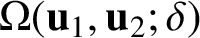 $\Omega (\mathbf {u}_{1},\mathbf {u}_{2};\delta )$
, and carrying out r consecutive
$\Omega (\mathbf {u}_{1},\mathbf {u}_{2};\delta )$
, and carrying out r consecutive
 $3$
-cycles of the area magnification process via shortlines, we obtain a new parallelogram
$3$
-cycles of the area magnification process via shortlines, we obtain a new parallelogram
 $\mathcal {P}^{(r)}$
on an X-face, or X-faces, such that one side is the vector
$\mathcal {P}^{(r)}$
on an X-face, or X-faces, such that one side is the vector
 $\delta \mathbf {u}^{(r)}_{1}$
, and the other side is the vector
$\delta \mathbf {u}^{(r)}_{1}$
, and the other side is the vector
 $\delta \mathbf {u}^{(r)}_{2}$
; see (4-10)–(4-13).
$\delta \mathbf {u}^{(r)}_{2}$
; see (4-10)–(4-13).
Of course, we are particularly interested in empty fundamental parallelograms
 $\mathcal {P}\in \Omega (\mathbf {u}_{1},\mathbf {u}_{2};\delta )$
.
$\mathcal {P}\in \Omega (\mathbf {u}_{1},\mathbf {u}_{2};\delta )$
.
5 Grids and iteration
We first establish the following geometric result which we use a few times.
Lemma 5.1 (‘area lemma’)
Let
 $\Omega $
be an arbitrary parallelogram lattice in
$\Omega $
be an arbitrary parallelogram lattice in
 $\mathbb {R}^{2}$
such that each fundamental parallelogram has diameter
$\mathbb {R}^{2}$
such that each fundamental parallelogram has diameter
 $\eta>0$
and area
$\eta>0$
and area
 $\Delta $
. Then a straight-line segment S with length
$\Delta $
. Then a straight-line segment S with length
 $L>0$
intersects at most
$L>0$
intersects at most
 $$ \begin{align*} \frac{2\eta(L+2\eta)}{\Delta} \end{align*} $$
fundamental parallelograms in
 $\Omega $
.
$\Omega $
.
On the other hand, let A be a convex set in
 $\mathbb{R}^2$
lying within an aligned square U of area 1.Then the boundary
$\mathbb{R}^2$
lying within an aligned square U of area 1.Then the boundary
 $\partial A$
of A intersects at most
$\partial A$
of A intersects at most
 $$ \begin{align*} 8\cdot\frac{2\eta(\sqrt{2}+2\eta)}{\Delta} \end{align*} $$
fundamental parallelograms in
 $\Omega$
.
$\Omega$
.
Proof. For any two points
 $P,Q\in \mathbb {R}^{2}$
, let
$P,Q\in \mathbb {R}^{2}$
, let
 $\rho (P,Q)$
denote the usual Euclidean distance between P and Q. For any
$\rho (P,Q)$
denote the usual Euclidean distance between P and Q. For any
 $\eta>0$
, consider the
$\eta>0$
, consider the
 $\eta $
-neighborhood of S given by
$\eta $
-neighborhood of S given by
 $$ \begin{align*} S(\eta)=\{P\in\mathbb{R}^2:\rho(P,Q)\leqslant\eta\mbox{ for some }Q\in S\}. \end{align*} $$
It is easy to see that
 $\operatorname {\mathrm {area}}(S(\eta ))\leqslant 2\eta (L+2\eta )$
. Note next that every fundamental parallelogram in
$\operatorname {\mathrm {area}}(S(\eta ))\leqslant 2\eta (L+2\eta )$
. Note next that every fundamental parallelogram in
 $\Omega $
that intersects S is completely contained in
$\Omega $
that intersects S is completely contained in
 $S(\eta )$
. Since each such fundamental parallelogram has area
$S(\eta )$
. Since each such fundamental parallelogram has area
 $\Delta $
, a simple calculation shows that the number of fundamental parallelograms in
$\Delta $
, a simple calculation shows that the number of fundamental parallelograms in
 $\Omega $
that intersect S does not exceed
$\Omega $
that intersect S does not exceed
 $$ \begin{align*} \frac{\operatorname{\mathrm{area}}(S(\eta))}{\Delta}\leqslant\frac{2\eta(L+2\eta)}{\Delta}. \end{align*} $$
The second assertion follows from the inequality
 $$ \begin{align*} \operatorname{\mathrm{area}}((\partial A)(\eta))\le\operatorname{\mathrm{area}}((\partial U)(\sqrt{2}\eta)), \end{align*} $$
where
 $\partial U$
denotes the boundary of U.
$\partial U$
denotes the boundary of U.
This completes the proof.
Throughout, we assume that
 $k\geqslant 8$
, so that
$k\geqslant 8$
, so that
 $\alpha _{k}<1/16$
.
$\alpha _{k}<1/16$
.
We need some notation.
First of all, we rewrite (4-20) in the form
 $$ \begin{align} \delta=\frac{\alpha_{k}^{3\ell/2}}{c_{1}}, \end{align} $$
where the constant
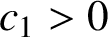 $c_{1}>0$
will be specified later. We also write
$c_{1}>0$
will be specified later. We also write
 $$ \begin{align*} \ell=r+(r-1)+(r-2)+\cdots+c_2=\frac{r(r+1)}{2}-\frac{(c_2-1)c_2}{2}, \end{align*} $$
where the constant
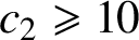 $c_{2}\geqslant 10$
will be specified later. More generally, for every integer
$c_{2}\geqslant 10$
will be specified later. More generally, for every integer
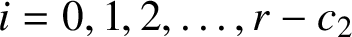 $i=0,1,2,\ldots ,r-c_{2}$
, we write
$i=0,1,2,\ldots ,r-c_{2}$
, we write
 $$ \begin{align} \ell_{i}=\sum_{h=0}^{i}(r-h)=\frac{r(r+1)}{2}-\frac{(r-i-1)(r-i)}{2}, \end{align} $$
so that, in particular,
 $$ \begin{align} \ell_{0}=r, \quad \ell_{1}=r+(r-1), \quad \ell_{r-c_{2}-1}=\ell-c_{2} \quad\mbox{and}\quad \ell_{r-c_{2}}=\ell, \end{align} $$
and let the integer
 $q_{i}$
satisfy the inequalities
$q_{i}$
satisfy the inequalities
 $$ \begin{align} \frac{c_{1}}{(r-i)^{4}}\alpha_{k}^{-3(\ell-\ell_{i})/2}-1<q_{i}\leqslant\frac{c_{1}}{(r-i)^{4}}\alpha_{k}^{-3(\ell-\ell_{i})/2}. \end{align} $$
In particular, the integer
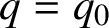 $q=q_{0}$
satisfies the inequalities
$q=q_{0}$
satisfies the inequalities
 $$ \begin{align} \frac{c_{1}}{r^{4}}\alpha_{k}^{-3(\ell-r)/2}-1<q\leqslant\frac{c_{1}}{r^{4}}\alpha_{k}^{-3(\ell-r)/2}. \end{align} $$
The calculations here and below makes use of the key fact that we can choose the value of the parameter
 $\ell $
as large as possible. It follows that
$\ell $
as large as possible. It follows that
 $r\approx \sqrt {2\ell }$
can also be arbitrarily large.
$r\approx \sqrt {2\ell }$
can also be arbitrarily large.
We are now ready to describe an iterative process that allows us to construct grids that contain empty fundamental parallelograms that are also nonsplitting during the magnification process.
Preparatory step. We begin our process with a
 $q\times q$
grid
$q\times q$
grid
 $\mathcal {G}$
of fundamental parallelograms
$\mathcal {G}$
of fundamental parallelograms
 $\mathcal {P}\in \Omega $
. Since each fundamental parallelogram
$\mathcal {P}\in \Omega $
. Since each fundamental parallelogram
 $\mathcal {P}\in \Omega $
has sides given by the vectors
$\mathcal {P}\in \Omega $
has sides given by the vectors
 $\delta \mathbf {u}_{1}$
and
$\delta \mathbf {u}_{1}$
and
 $\delta \mathbf {u}_{2}$
, a
$\delta \mathbf {u}_{2}$
, a
 $q\times q$
grid
$q\times q$
grid
 $\mathcal {G}$
consists of
$\mathcal {G}$
consists of
 $q^{2}$
fundamental parallelograms
$q^{2}$
fundamental parallelograms
 $\mathcal {P}\in \Omega $
and is itself a larger parallelogram with sides given by the vectors
$\mathcal {P}\in \Omega $
and is itself a larger parallelogram with sides given by the vectors
 $q\delta \mathbf {u}_{1}$
and
$q\delta \mathbf {u}_{1}$
and
 $q\delta \mathbf {u}_{2}$
.
$q\delta \mathbf {u}_{2}$
.
Consider a parallelogram lattice
 $\mathcal {H}$
that contains an X-face, with grid fundamental parallelograms given by
$\mathcal {H}$
that contains an X-face, with grid fundamental parallelograms given by
 $q\times q$
grids
$q\times q$
grids
 $\mathcal {G}$
with sides given by the vectors
$\mathcal {G}$
with sides given by the vectors
 $q\delta \mathbf {u}_{1}$
and
$q\delta \mathbf {u}_{1}$
and
 $q\delta \mathbf {u}_{2}$
.
$q\delta \mathbf {u}_{2}$
.
Remark 5.2. Here we use the term grid fundamental parallelograms to distinguish these larger parallelograms from the fundamental parallelograms
 $\mathcal {P}\in \Omega $
.
$\mathcal {P}\in \Omega $
.
It follows easily from (4-7)–(4-9) that the diameter of each grid fundamental parallelogram in
 $\mathcal {H}$
does not exceed
$\mathcal {H}$
does not exceed
 $$ \begin{align} 8q\delta\leqslant\frac{8\alpha_{k}^{3r/2}}{r^{4}}\leqslant\frac{1}{2r^{4}}, \end{align} $$
in view of (5-1), (5-5) and the assumption on k. This is extremely small when r is large, and ensures that there are many
 $q\times q$
grids
$q\times q$
grids
 $\mathcal {G}$
that are completely contained in an X-face of
$\mathcal {G}$
that are completely contained in an X-face of
 $X_{0}$
. It also follows easily from (4-14) that each grid fundamental parallelogram in
$X_{0}$
. It also follows easily from (4-14) that each grid fundamental parallelogram in
 $\mathcal {H}$
has area
$\mathcal {H}$
has area
 $\Delta =(4+o_{k}(1))q^{2}\delta ^{2}\alpha _{k}^{1/2}$
. On the other hand, an X-face has four boundary edges, each with unit length. Applying Lemma 5.1, we conclude that the number of grid fundamental parallelograms in
$\Delta =(4+o_{k}(1))q^{2}\delta ^{2}\alpha _{k}^{1/2}$
. On the other hand, an X-face has four boundary edges, each with unit length. Applying Lemma 5.1, we conclude that the number of grid fundamental parallelograms in
 $\mathcal {H}$
that intersect the boundary of any of the three X-faces in
$\mathcal {H}$
that intersect the boundary of any of the three X-faces in
 $X_{0}$
does not exceed
$X_{0}$
does not exceed
 $$ \begin{align*} 3\cdot4\cdot\frac{16q\delta(1+16q\delta)}{(4+o_k(1))q^2\delta^2\alpha_k^{1/2}}=\frac{48+o_k(1)}{q\delta\alpha_k^{1/2}}. \end{align*} $$
The total number of fundamental parallelograms
 $\mathcal {P}\in \Omega $
is roughly equal to
$\mathcal {P}\in \Omega $
is roughly equal to
 $$ \begin{align*} \frac{3q^2}{(4+o_k(1))q^2\delta^2\alpha_k^{1/2}}, \end{align*} $$
so it follows from (4-24) and (5-6) that the total number of empty fundamental parallelograms
 $\mathcal {P}\in \Omega $
contained in
$\mathcal {P}\in \Omega $
contained in
 $q\times q$
grids
$q\times q$
grids
 $\mathcal {G}$
that do not intersect the boundary of any of the three X-faces in
$\mathcal {G}$
that do not intersect the boundary of any of the three X-faces in
 $X_{0}$
is at least
$X_{0}$
is at least
 $$ \begin{align*} &\frac{3q^{2}}{(4+o_{k}(1))q^{2}\delta^{2}\alpha_{k}^{1/2}}\cdot\frac{\tau-\varepsilon}{20}-\frac{(48+o_{k}(1))q^{2}}{q\delta\alpha_{k}^{1/2}}\\ &\quad=\frac{3}{(4+o_{k}(1))q^{2}\delta^{2}\alpha_{k}^{1/2}}\Bigg(\frac{\tau - \epsilon}{20}-(64+o_{k}(1))q\delta\Bigg)q^{2}. \end{align*} $$
Thus, the average proportion of empty fundamental parallelograms in a
 $q\times q$
grid
$q\times q$
grid
 $\mathcal {G}$
that does not intersect the boundary of any of the three X-faces in
$\mathcal {G}$
that does not intersect the boundary of any of the three X-faces in
 $X_{0}$
is at least
$X_{0}$
is at least
 $$ \begin{align*} \frac{\tau-\varepsilon}{20}-(64+o_k(1))q\delta. \end{align*} $$
Note that it follows from (5-6) that
 $$ \begin{align*} (64+o_k(1))q\delta\leqslant\frac{4}{r^4}<\frac{\tau}{100r^2} \end{align*} $$
for large r.
We now choose a
 $q\times q$
grid
$q\times q$
grid
 $\mathcal {G}_{0}$
that is completely contained in an X-face of
$\mathcal {G}_{0}$
that is completely contained in an X-face of
 $X_{0}$
and contains the maximum number of empty fundamental parallelograms
$X_{0}$
and contains the maximum number of empty fundamental parallelograms
 $\mathcal {P}\in \Omega $
. Clearly the proportion of empty fundamental parallelograms
$\mathcal {P}\in \Omega $
. Clearly the proportion of empty fundamental parallelograms
 $\mathcal {P}\in \mathcal {G}_{0}$
is at least
$\mathcal {P}\in \mathcal {G}_{0}$
is at least
 $$ \begin{align} \tau_{0}=\frac{\tau-\varepsilon}{20}-\frac{\tau}{100r^{2}}. \end{align} $$
Initial step. Starting with
 $\mathcal {G}_{0}$
and applying the first
$\mathcal {G}_{0}$
and applying the first
 $3$
-cycle of magnifications
$3$
-cycle of magnifications
 $$ \begin{align*} X_0 \mathop{\longrightarrow}\limits^{\mathbf{v}_1}Y_0 \mathop{\longrightarrow}\limits^{\mathbf{v}_2}Z_0 \mathop{\longrightarrow}\limits^{\mathbf{v}_0}X_0, \end{align*} $$
where
 $$ \begin{align*} Y_0=Y_1\cup Y_2\cup Y_3 \quad\mbox{and}\quad Z_0=Z_1\cup Z_2\cup Z_5 \end{align*} $$
as shown in Figures 4 and 5, we obtain a magnified
 $q\times q$
grid
$q\times q$
grid
 $\mathcal {G}_{0}^{(1)}$
. Employing this argument r times in succession, we obtain a magnified
$\mathcal {G}_{0}^{(1)}$
. Employing this argument r times in succession, we obtain a magnified
 $q\times q$
grid
$q\times q$
grid
 $\mathcal {G}_{0}^{(r)}=\mathcal {G}_{0}^{(\ell _{0})}$
at the end of r consecutive
$\mathcal {G}_{0}^{(r)}=\mathcal {G}_{0}^{(\ell _{0})}$
at the end of r consecutive
 $3$
-cycles of magnifications. At each magnification, the diameter of the parallelogram grows by a factor
$3$
-cycles of magnifications. At each magnification, the diameter of the parallelogram grows by a factor
 $\alpha _{k}^{-1/2}$
, so that the diameter of the parallelogram at each stage of the
$\alpha _{k}^{-1/2}$
, so that the diameter of the parallelogram at each stage of the
 $3r$
-step magnification process, assuming that no splitting takes place, never exceeds
$3r$
-step magnification process, assuming that no splitting takes place, never exceeds
 $$ \begin{align} 8q\delta\alpha_{k}^{-3r/2}\leqslant\frac{8}{r^{4}}\leqslant1, \end{align} $$
in view of (5-6), as long as
 $r\geqslant 2$
. If splitting occurs at any step of the magnification process, the bound (5-8) on the diameter guarantees that the image splits into at most four convex parts, each contained in a square face. For convenience, we call these convex square-parts.
$r\geqslant 2$
. If splitting occurs at any step of the magnification process, the bound (5-8) on the diameter guarantees that the image splits into at most four convex parts, each contained in a square face. For convenience, we call these convex square-parts.
Remark 5.3. Note that the L-solid has only
 $14$
square faces in total. This number is reduced to nine with face identification. Thus, many distinct convex square-parts may fall into the same square face. However, we need to exercise care and treat each separately.
$14$
square faces in total. This number is reduced to nine with face identification. Thus, many distinct convex square-parts may fall into the same square face. However, we need to exercise care and treat each separately.
Since there are
 $3r$
steps in the magnification process, it follows that the
$3r$
steps in the magnification process, it follows that the
 $q\times q$
grid
$q\times q$
grid
 $\mathcal {G}_{0}^{(r)}$
splits into
$\mathcal {G}_{0}^{(r)}$
splits into
 $R\leqslant 4^{3r}$
convex square-parts.
$R\leqslant 4^{3r}$
convex square-parts.
Let A be a convex square-part of
 $\mathcal {G}_{0}^{(r)}$
, and suppose that it is contained in the unit square face U.
$\mathcal {G}_{0}^{(r)}$
, and suppose that it is contained in the unit square face U.
Suppose first of all that A contains a vertex
 $P_{0}$
of
$P_{0}$
of
 $\mathcal {G}_{0}^{(r)}$
. We consider a parallelogram lattice
$\mathcal {G}_{0}^{(r)}$
. We consider a parallelogram lattice
 $\mathcal {H}_{0}$
, where
$\mathcal {H}_{0}$
, where
 $P_{0}$
is one of the vertices and a grid fundamental parallelogram in
$P_{0}$
is one of the vertices and a grid fundamental parallelogram in
 $\mathcal {H}_{0}$
has sides given by the vectors
$\mathcal {H}_{0}$
has sides given by the vectors
 $q_{1}\delta \mathbf {u}_{1}^{(r)}$
and
$q_{1}\delta \mathbf {u}_{1}^{(r)}$
and
 $q_{1}\delta \mathbf {u}_{2}^{(r)}$
. We say that a grid fundamental parallelogram in
$q_{1}\delta \mathbf {u}_{2}^{(r)}$
. We say that a grid fundamental parallelogram in
 $\mathcal {H}_{0}$
is good if it is completely inside A, and bad if it intersects the boundary of A. Those grid fundamental parallelograms that do not intersect A are irrelevant to our discussion.
$\mathcal {H}_{0}$
is good if it is completely inside A, and bad if it intersects the boundary of A. Those grid fundamental parallelograms that do not intersect A are irrelevant to our discussion.
Meanwhile, it follows from (4-16) that the diameter
 $\eta $
of each grid fundamental parallelogram in
$\eta $
of each grid fundamental parallelogram in
 $\mathcal {H}_{0}$
satisfies
$\mathcal {H}_{0}$
satisfies
 $$ \begin{align*} \eta\leqslant8q_1\delta\alpha_k^{-3r/2}, \end{align*} $$
and it follows from (4-15) that each grid fundamental parallelogram in
 $\mathcal {H}_{0}$
has area
$\mathcal {H}_{0}$
has area
 $$ \begin{align*} \Delta=(4+o_k(1))q_1^2\delta^2\alpha_k^{-3r}\alpha_k^{1/2}. \end{align*} $$
Applying Lemma 5.1, we conclude that there are at most
 $$ \begin{align} 8\cdot\frac{16q_{1}\delta\alpha_{k}^{-3r/2}(\sqrt{2}+16q_{1}\delta\alpha_{k}^{-3r/2})}{(4+o_{k}(1))q_{1}^{2}\delta^{2}\alpha_{k}^{-3r}\alpha_{k}^{1/2}} \leqslant\frac{64+o_{k}(1)}{q_{1}\delta\alpha_{k}^{-3r/2}\alpha_{k}^{1/2}} \end{align} $$
bad grid fundamental parallelograms in
 $\mathcal {H}_{0}$
that intersect the convex square-part A of
$\mathcal {H}_{0}$
that intersect the convex square-part A of
 $\mathcal {G}_{0}^{(r)}$
.
$\mathcal {G}_{0}^{(r)}$
.
Suppose next that A does not contain a vertex
 $P_{0}$
of
$P_{0}$
of
 $\mathcal {G}_{0}^{(r)}$
. Then A is small, and we can consider an arbitrary parallelogram lattice
$\mathcal {G}_{0}^{(r)}$
. Then A is small, and we can consider an arbitrary parallelogram lattice
 $\mathcal {H}_{0}$
with sides given by the vectors
$\mathcal {H}_{0}$
with sides given by the vectors
 $q_{1}\delta \mathbf {u}_{1}^{(r)}$
and
$q_{1}\delta \mathbf {u}_{1}^{(r)}$
and
 $q_{1}\delta \mathbf {u}_{2}^{(r)}$
. An analogous argument shows that the estimate (5-9) remains valid.
$q_{1}\delta \mathbf {u}_{2}^{(r)}$
. An analogous argument shows that the estimate (5-9) remains valid.
There are at most
 $4^{3r}$
convex square-parts of
$4^{3r}$
convex square-parts of
 $\mathcal {G}_{0}^{(r)}$
. It follows that the total number of bad grid fundamental parallelograms that intersect any convex square-part of
$\mathcal {G}_{0}^{(r)}$
. It follows that the total number of bad grid fundamental parallelograms that intersect any convex square-part of
 $\mathcal {G}_{0}^{(r)}$
is at most
$\mathcal {G}_{0}^{(r)}$
is at most
 $$ \begin{align*} 4^{3r}\cdot\frac{64+o_k(1)}{q_1\delta\alpha_k^{-3r/2}\alpha_k^{1/2}}, \end{align*} $$
and so the total number of fundamental parallelograms
 $\mathcal {P}^{(r)}\in \mathcal {G}_{0}^{(r)}$
contained in bad grid fundamental parallelograms in
$\mathcal {P}^{(r)}\in \mathcal {G}_{0}^{(r)}$
contained in bad grid fundamental parallelograms in
 $\mathcal {G}_{0}^{(r)}$
is at most
$\mathcal {G}_{0}^{(r)}$
is at most
 $$ \begin{align*} 4^{3r}\cdot\frac{(64+o_k(1))q_1^2}{q_1\delta\alpha_k^{-3r/2}\alpha_k^{1/2}}. \end{align*} $$
Now the total number of fundamental parallelograms
 $\mathcal {P}^{(r)}\in \mathcal {G}_{0}^{(r)}$
is equal to
$\mathcal {P}^{(r)}\in \mathcal {G}_{0}^{(r)}$
is equal to
 $q^{2}$
. On the other hand, since the magnified image of an empty set is empty, the proportion of empty fundamental parallelograms
$q^{2}$
. On the other hand, since the magnified image of an empty set is empty, the proportion of empty fundamental parallelograms
 $\mathcal {P}^{(r)}\in \mathcal {G}_{0}^{(r)}$
is at least
$\mathcal {P}^{(r)}\in \mathcal {G}_{0}^{(r)}$
is at least
 $\tau _{0}$
, which is given by (5-7). Hence, the total number of empty fundamental parallelograms
$\tau _{0}$
, which is given by (5-7). Hence, the total number of empty fundamental parallelograms
 $\mathcal {P}^{(r)}\in \mathcal {G}_{0}^{(r)}$
contained in good grid fundamental parallelograms in
$\mathcal {P}^{(r)}\in \mathcal {G}_{0}^{(r)}$
contained in good grid fundamental parallelograms in
 $\mathcal {G}_{0}^{(r)}$
is at least
$\mathcal {G}_{0}^{(r)}$
is at least
 $$ \begin{align*} q^2\tau_0-4^{3r}\cdot\frac{(64+o_k(1))q_1^2}{q_1\delta\alpha_k^{-3r/2}\alpha_k^{1/2}}. \end{align*} $$
Thus, the average proportion of empty fundamental parallelograms in a good
 $q_{1}\times q_{1}$
grid fundamental parallelogram in
$q_{1}\times q_{1}$
grid fundamental parallelogram in
 $\mathcal {G}_{0}^{(r)}$
is at least
$\mathcal {G}_{0}^{(r)}$
is at least
 $$ \begin{align*} \tau_0-\frac{4^{3r}}{q^2}\cdot\frac{(64+o_k(1))q_1^2}{q_1\delta\alpha_k^{-3r/2}\alpha_k^{1/2}}. \end{align*} $$
Note that it follows from (5-1) and (5-3)–(5-5) that
 $$ \begin{align*} \frac{4^{3r}}{q^2}\cdot\frac{(64+o_k(1))q_1^2}{q_1\delta\alpha_k^{-3r/2}\alpha_k^{1/2}} =\frac{(64+o_k(1))}{(r-1)^4}\alpha_k^{-2}(4\alpha_k^{1/2})^{3r}r^8 <\frac{\tau}{100(r-1)^2} \end{align*} $$
for large r.
We now choose a
 $q_{1}\times q_{1}$
grid
$q_{1}\times q_{1}$
grid
 $\mathcal {G}_{1}$
which is a good grid fundamental parallelogram in
$\mathcal {G}_{1}$
which is a good grid fundamental parallelogram in
 $\mathcal {G}_{0}^{(\ell _{0})}=\mathcal {G}_{0}^{(r)}$
and which contains the maximum number of empty fundamental parallelograms
$\mathcal {G}_{0}^{(\ell _{0})}=\mathcal {G}_{0}^{(r)}$
and which contains the maximum number of empty fundamental parallelograms
 $\mathcal {P}^{(\ell _{0})}=\mathcal {P}^{(r)}$
which are images of
$\mathcal {P}^{(\ell _{0})}=\mathcal {P}^{(r)}$
which are images of
 $\mathcal {P}\in \mathcal {G}_{0}$
. Clearly the proportion of empty fundamental parallelograms
$\mathcal {P}\in \mathcal {G}_{0}$
. Clearly the proportion of empty fundamental parallelograms
 $\mathcal {P}^{(\ell _{0})}=\mathcal {P}^{(r)}\in \mathcal {G}_{1}$
is at least
$\mathcal {P}^{(\ell _{0})}=\mathcal {P}^{(r)}\in \mathcal {G}_{1}$
is at least
 $$ \begin{align} \tau_{1}=\tau_{0}-\frac{\tau}{100(r-1)^{2}}. \end{align} $$
Furthermore, since the image
 $\mathcal {P}^{(\ell _{0})}=\mathcal {P}^{(r)}$
of the fundamental parallelogram
$\mathcal {P}^{(\ell _{0})}=\mathcal {P}^{(r)}$
of the fundamental parallelogram
 $\mathcal {P}$
under the
$\mathcal {P}$
under the
 $3\ell _{0}=3r$
magnifications is completely inside a convex square-part of
$3\ell _{0}=3r$
magnifications is completely inside a convex square-part of
 $\mathcal {G}_{0}^{(\ell _{0})}=\mathcal {G}_{0}^{(r)}$
,
$\mathcal {G}_{0}^{(\ell _{0})}=\mathcal {G}_{0}^{(r)}$
,
 $\mathcal {P}$
never splits during the
$\mathcal {P}$
never splits during the
 $3\ell _{0}=3r$
magnifications. In particular, these empty fundamental parallelograms are nonsplitting.
$3\ell _{0}=3r$
magnifications. In particular, these empty fundamental parallelograms are nonsplitting.
Inductive step. Suppose, in general, that
 $\mathcal {G}_{i}$
is
$\mathcal {G}_{i}$
is
 $q_{i}\times q_{i}$
grid which is a good grid fundamental parallelogram, contained in a convex square-part of
$q_{i}\times q_{i}$
grid which is a good grid fundamental parallelogram, contained in a convex square-part of
 $\mathcal {G}_{0}^{(\ell _{i-1})}=\mathcal {G}_{i-1}^{(r-i+1)}$
, and that the proportion of empty and nonsplitting fundamental parallelograms
$\mathcal {G}_{0}^{(\ell _{i-1})}=\mathcal {G}_{i-1}^{(r-i+1)}$
, and that the proportion of empty and nonsplitting fundamental parallelograms
 $\mathcal {P}^{(\ell _{i-1})}\in \mathcal {G}_{i}$
is at least
$\mathcal {P}^{(\ell _{i-1})}\in \mathcal {G}_{i}$
is at least
 $$ \begin{align} \tau_{i}=\tau_{i-1}-\frac{\tau}{100(r-i)^{2}}, \end{align} $$
where
 $\mathcal {P}^{(\ell _{i-1})}$
represents the image of
$\mathcal {P}^{(\ell _{i-1})}$
represents the image of
 $\mathcal {P}$
under
$\mathcal {P}$
under
 $3\ell _{i-1}$
magnifications, remaining empty and nonsplitting during the entire process
$3\ell _{i-1}$
magnifications, remaining empty and nonsplitting during the entire process
 $\mathcal {G}_{0}\to \mathcal {G}_{i}$
.
$\mathcal {G}_{0}\to \mathcal {G}_{i}$
.
Starting with
 $\mathcal {G}_{i}$
and applying the first
$\mathcal {G}_{i}$
and applying the first
 $3$
-cycle of magnifications
$3$
-cycle of magnifications
 $$ \begin{align*} X_0 \mathop{\longrightarrow}\limits^{\mathbf{v}_1}Y_0 \mathop{\longrightarrow}\limits^{\mathbf{v}_2}Z_0 \mathop{\longrightarrow}\limits^{\mathbf{v}_0}X_0, \end{align*} $$
we now obtain a magnified
 $q_{i}\times q_{i}$
grid
$q_{i}\times q_{i}$
grid
 $\mathcal {G}_{i}^{(1)}$
. Employing this argument
$\mathcal {G}_{i}^{(1)}$
. Employing this argument
 $r-i$
times in succession, we obtain a magnified
$r-i$
times in succession, we obtain a magnified
 $q_{i}\times q_{i}$
grid
$q_{i}\times q_{i}$
grid
 $\mathcal {G}_{i}^{(r-1)}=\mathcal {G}_{0}^{(\ell _{i})}$
at the end of
$\mathcal {G}_{i}^{(r-1)}=\mathcal {G}_{0}^{(\ell _{i})}$
at the end of
 $r-i$
consecutive
$r-i$
consecutive
 $3$
-cycles of magnifications. The diameter of the grid
$3$
-cycles of magnifications. The diameter of the grid
 $\mathcal {G}_{i}$
is clearly bounded by
$\mathcal {G}_{i}$
is clearly bounded by
 $8q_{i}\delta \alpha _{k}^{-3\ell _{i-1}/2}$
. At each magnification, the diameter of the parallelogram grows by a factor
$8q_{i}\delta \alpha _{k}^{-3\ell _{i-1}/2}$
. At each magnification, the diameter of the parallelogram grows by a factor
 $\alpha _{k}^{-1/2}$
, so that the diameter of the parallelogram at each stage of the present
$\alpha _{k}^{-1/2}$
, so that the diameter of the parallelogram at each stage of the present
 $3(r-i)$
-step magnification process, assuming that no splitting takes place, never exceeds
$3(r-i)$
-step magnification process, assuming that no splitting takes place, never exceeds
 $$ \begin{align} 8q_{i}\delta\alpha_{k}^{-3\ell_{i-1}/2}\alpha_{k}^{-3(r-i)/2} =8q_{i}\delta\alpha_{k}^{-3\ell_{i}/2} \leqslant\frac{8}{(r-i)^{4}}\leqslant1, \end{align} $$
in view of (5-1) and (5-4), as long as
 $r-i\geqslant 2$
. If splitting occurs at any step of the magnification process, the bound (5-12) on the diameter guarantees that the image splits into at most four convex square-parts, each contained in a square face. Since there are
$r-i\geqslant 2$
. If splitting occurs at any step of the magnification process, the bound (5-12) on the diameter guarantees that the image splits into at most four convex square-parts, each contained in a square face. Since there are
 $3(r-i)$
steps in the magnification process, it follows that the
$3(r-i)$
steps in the magnification process, it follows that the
 $q_{i}\times q_{i}$
grid
$q_{i}\times q_{i}$
grid
 $\mathcal {G}_{i}^{(r-i)}$
splits into
$\mathcal {G}_{i}^{(r-i)}$
splits into
 $R_{i}\leqslant 4^{3(r-i)}$
convex square-parts.
$R_{i}\leqslant 4^{3(r-i)}$
convex square-parts.
Let A be a convex square-part of
 $\mathcal {G}_{i}^{(r-i)}$
, and suppose that it is contained in the unit square face U. We may suppose that A contains a vertex
$\mathcal {G}_{i}^{(r-i)}$
, and suppose that it is contained in the unit square face U. We may suppose that A contains a vertex
 $P_{0}$
of
$P_{0}$
of
 $\mathcal {G}_{0}^{(r)}$
, as the argument in the alternative case requires only minor modifications. We consider a parallelogram lattice
$\mathcal {G}_{0}^{(r)}$
, as the argument in the alternative case requires only minor modifications. We consider a parallelogram lattice
 $\mathcal {H}_{i}$
, where
$\mathcal {H}_{i}$
, where
 $P_{0}$
is one of the vertices and a grid fundamental parallelogram in
$P_{0}$
is one of the vertices and a grid fundamental parallelogram in
 $\mathcal {H}_{i}$
has sides given by the vectors
$\mathcal {H}_{i}$
has sides given by the vectors
 $q_{i+1}\delta \mathbf {u}_{1}^{(\ell _{i})}$
and
$q_{i+1}\delta \mathbf {u}_{1}^{(\ell _{i})}$
and
 $q_{i+1}\delta \mathbf {u}_{2}^{(\ell _{i})}$
. We say that a grid fundamental parallelogram in
$q_{i+1}\delta \mathbf {u}_{2}^{(\ell _{i})}$
. We say that a grid fundamental parallelogram in
 $\mathcal {H}_{i}$
is good if it is completely inside A, and bad if it intersects the boundary of A. Those grid fundamental parallelograms that do not intersect A are irrelevant to our discussion.
$\mathcal {H}_{i}$
is good if it is completely inside A, and bad if it intersects the boundary of A. Those grid fundamental parallelograms that do not intersect A are irrelevant to our discussion.
Meanwhile, it follows from (4-16) that the diameter
 $\eta $
of each grid fundamental parallelogram in
$\eta $
of each grid fundamental parallelogram in
 $\mathcal {H}_{i}$
satisfies
$\mathcal {H}_{i}$
satisfies
 $$ \begin{align*} \eta\leqslant8q_{i+1}\delta\alpha_k^{-3\ell_i/2}, \end{align*} $$
and it follows from (4-15) that each grid fundamental parallelogram in
 $\mathcal {H}_{0}^{(r)}$
has area
$\mathcal {H}_{0}^{(r)}$
has area
 $$ \begin{align*} \Delta=(4+o_k(1))q_{i+1}^2\delta^2\alpha_k^{-3\ell_i}\alpha_k^{1/2}. \end{align*} $$
Applying Lemma 5.1, we conclude that there are at most
 $$ \begin{align*} 8\cdot\frac{16q_{i+1}\delta\alpha_k^{-3\ell_i/2}(\sqrt{2}+16q_{i+1}\delta\alpha_k^{-3\ell_i/2})} {(4+o_k(1))q_{i+1}^2\delta^2\alpha_k^{-3\ell_i}\alpha_k^{1/2}} \leqslant\frac{64+o_k(1)}{q_{i+1}\delta\alpha_k^{-3\ell_i/2}\alpha_k^{1/2}} \end{align*} $$
bad grid fundamental parallelograms in
 $\mathcal {H}_{i}$
that intersect the convex square-part A of
$\mathcal {H}_{i}$
that intersect the convex square-part A of
 $\mathcal {G}_{i}^{(r-i)}$
.
$\mathcal {G}_{i}^{(r-i)}$
.
There are at most
 $4^{3(r-i)}$
convex square-parts of
$4^{3(r-i)}$
convex square-parts of
 $\mathcal {G}_{i}^{(r-i)}$
. It follows that the total number of bad grid fundamental parallelograms that intersect any convex square-part of
$\mathcal {G}_{i}^{(r-i)}$
. It follows that the total number of bad grid fundamental parallelograms that intersect any convex square-part of
 $\mathcal {G}_{i}^{(r-i)}$
is at most
$\mathcal {G}_{i}^{(r-i)}$
is at most
 $$ \begin{align*} 4^{3(r-i)}\cdot\frac{64+o_k(1)}{q_{i+1}\delta\alpha_k^{-3\ell_i/2}\alpha_k^{1/2}}, \end{align*} $$
and so the total number of fundamental parallelograms
 $\mathcal {P}^{(\ell _{i})}\in \mathcal {G}_{i}^{(r-i)}$
contained in bad grid fundamental parallelograms in
$\mathcal {P}^{(\ell _{i})}\in \mathcal {G}_{i}^{(r-i)}$
contained in bad grid fundamental parallelograms in
 $\mathcal {G}_{i}^{(r-i)}$
is at most
$\mathcal {G}_{i}^{(r-i)}$
is at most
 $$ \begin{align*} 4^{3(r-i)}\cdot\frac{(64+o_k(1))q_{i+1}^2}{q_{i+1}\delta\alpha_k^{-3\ell_i/2}\alpha_k^{1/2}}. \end{align*} $$
Now the total number of fundamental parallelograms
 $\mathcal {P}^{(\ell _{i})}\in \mathcal {G}_{i}^{(r-i)}$
is equal to
$\mathcal {P}^{(\ell _{i})}\in \mathcal {G}_{i}^{(r-i)}$
is equal to
 $q_{i}^{2}$
. On the other hand, since the magnified image of an empty set is empty, the proportion of empty fundamental parallelograms
$q_{i}^{2}$
. On the other hand, since the magnified image of an empty set is empty, the proportion of empty fundamental parallelograms
 $\mathcal {P}^{(\ell _{i})}\in \mathcal {G}_{i}^{(r-i)}$
is at least
$\mathcal {P}^{(\ell _{i})}\in \mathcal {G}_{i}^{(r-i)}$
is at least
 $\tau _{i}$
given by (5-11). Hence, the total number of empty fundamental parallelograms
$\tau _{i}$
given by (5-11). Hence, the total number of empty fundamental parallelograms
 $\mathcal {P}^{(\ell _{i})}\in \mathcal {G}_{i}^{(r-i)}$
contained in good grid fundamental parallelograms in
$\mathcal {P}^{(\ell _{i})}\in \mathcal {G}_{i}^{(r-i)}$
contained in good grid fundamental parallelograms in
 $\mathcal {G}_{i}^{(r-i)}$
is at least
$\mathcal {G}_{i}^{(r-i)}$
is at least
 $$ \begin{align*} q_i^2\tau_i-4^{3(r-i)}\cdot\frac{(64+o_k(1))q_{i+1}^2}{q_{i+1}\delta\alpha_k^{-3\ell_i/2}\alpha_k^{1/2}}. \end{align*} $$
It follows that the average proportion of empty fundamental parallelograms in a good
 $q_{i+1}\times q_{i+1}$
grid fundamental parallelogram in
$q_{i+1}\times q_{i+1}$
grid fundamental parallelogram in
 $\mathcal {G}_{i}^{(r-i)}$
is at least
$\mathcal {G}_{i}^{(r-i)}$
is at least
 $$ \begin{align*} \tau_i-\frac{4^{3(r-i)}}{q_i^2}\cdot\frac{(64+o_k(1))q_{i+1}^2}{q_{i+1}\delta\alpha_k^{-3\ell_i/2}\alpha_k^{1/2}}. \end{align*} $$
Note that it follows from (5-1), (5-2) and (5-4) that
 $$ \begin{align*} \frac{4^{3(r-i)}}{q_{i}^{2}}\cdot\frac{(64+o_{k}(1))q_{i+1}^{2}}{q_{i+1}\delta\alpha_{k}^{-3\ell_{i}/2}\alpha_{k}^{1/2}} &=\frac{(64+o_{k}(1))}{(r-i-1)^{4}}\alpha_{k}^{-2}(4\alpha_{k}^{1/2})^{3(r-i)}(r-i)^{8}\\ &<\frac{\tau}{100(r-i-1)^{2}} \end{align*} $$
for large
 $r-i$
. Since
$r-i$
. Since
 $r-i\geqslant c_{2}$
, we can choose
$r-i\geqslant c_{2}$
, we can choose
 $c_{2}$
sufficiently large so that
$c_{2}$
sufficiently large so that
 $$ \begin{align*} \alpha_k^{-2}(4\alpha_k^{1/2})^{3(r-i)}(r-i)^8\leqslant1 \end{align*} $$
whenever
 $r-i\geqslant c_{2}$
, for instance.
$r-i\geqslant c_{2}$
, for instance.
We can now choose a
 $q_{i+1}\times q_{i+1}$
grid
$q_{i+1}\times q_{i+1}$
grid
 $\mathcal {G}_{i+1}$
which is a good grid fundamental parallelogram in
$\mathcal {G}_{i+1}$
which is a good grid fundamental parallelogram in
 $\mathcal {G}_{0}^{(\ell _{i})}=\mathcal {G}_{i}^{(r-i)}$
and which contains the maximum number of empty fundamental parallelograms
$\mathcal {G}_{0}^{(\ell _{i})}=\mathcal {G}_{i}^{(r-i)}$
and which contains the maximum number of empty fundamental parallelograms
 $\mathcal {P}^{(\ell _{i})}$
which are images of
$\mathcal {P}^{(\ell _{i})}$
which are images of
 $\mathcal {P}\in \mathcal {G}_{0}$
. Clearly the proportion of empty fundamental parallelograms
$\mathcal {P}\in \mathcal {G}_{0}$
. Clearly the proportion of empty fundamental parallelograms
 $\mathcal {P}^{(\ell _{i})}\in \mathcal {G}_{i+1}$
is at least
$\mathcal {P}^{(\ell _{i})}\in \mathcal {G}_{i+1}$
is at least
 $$ \begin{align*} \tau_{i+1}=\tau_i-\frac{\tau}{100(r-i-1)^2}. \end{align*} $$
Furthermore, since the image
 $\mathcal {P}^{(\ell _{i})}$
of the fundamental parallelogram
$\mathcal {P}^{(\ell _{i})}$
of the fundamental parallelogram
 $\mathcal {P}$
under the
$\mathcal {P}$
under the
 $3\ell _{i}$
magnifications is completely inside a convex square-part of
$3\ell _{i}$
magnifications is completely inside a convex square-part of
 $\mathcal {G}_{0}^{(\ell _{i})}=\mathcal {G}_{i}^{(r-i)}$
,
$\mathcal {G}_{0}^{(\ell _{i})}=\mathcal {G}_{i}^{(r-i)}$
,
 $\mathcal {P}$
never splits during the
$\mathcal {P}$
never splits during the
 $3\ell _{i}$
magnifications from the very beginning. In particular, these empty fundamental parallelograms are nonsplitting.
$3\ell _{i}$
magnifications from the very beginning. In particular, these empty fundamental parallelograms are nonsplitting.
Last step. The final step of this iterative process concerns
 $i=r-c_{2}-1$
, with
$i=r-c_{2}-1$
, with
 $\ell _{i}=\ell -c_{2}$
. We conclude that we can choose an
$\ell _{i}=\ell -c_{2}$
. We conclude that we can choose an
 $(r-c_{2})\times (r-c_{2})$
grid
$(r-c_{2})\times (r-c_{2})$
grid
 $\mathcal {G}_{r-c_{2}}$
which is a good grid fundamental parallelogram in
$\mathcal {G}_{r-c_{2}}$
which is a good grid fundamental parallelogram in
 $\mathcal {G}_{0}^{(\ell -c_{2})}=\mathcal {G}_{r-c_{2}-1}^{(c_{2}+1)}$
, and the proportion of empty and parallelograms
$\mathcal {G}_{0}^{(\ell -c_{2})}=\mathcal {G}_{r-c_{2}-1}^{(c_{2}+1)}$
, and the proportion of empty and parallelograms
 $\mathcal {P}^{(\ell -c_{2})}\in \mathcal {G}_{r-c_{2}}$
is at least
$\mathcal {P}^{(\ell -c_{2})}\in \mathcal {G}_{r-c_{2}}$
is at least
 $$ \begin{align} \tau_{r-c_{2}}=\tau_{r-c_{2}-1}-\frac{\tau}{100c_{2}^{2}}. \end{align} $$
Furthermore, since the image
 $\mathcal {P}^{(\ell -c_{2})}$
of the fundamental parallelogram
$\mathcal {P}^{(\ell -c_{2})}$
of the fundamental parallelogram
 $\mathcal {P}$
under the
$\mathcal {P}$
under the
 $3(\ell -c_{2})$
magnifications is completely inside a convex square-part of
$3(\ell -c_{2})$
magnifications is completely inside a convex square-part of
 $\mathcal {G}_{0}^{(\ell -c_{2})}$
,
$\mathcal {G}_{0}^{(\ell -c_{2})}$
,
 $\mathcal {P}$
never splits during the
$\mathcal {P}$
never splits during the
 $3(\ell -c_{2})$
magnifications from the very beginning. In particular, these empty fundamental parallelograms are nonsplitting.
$3(\ell -c_{2})$
magnifications from the very beginning. In particular, these empty fundamental parallelograms are nonsplitting.
Combining (5-7), (5-10), (5-11) and (5-13), we see that
 $$ \begin{align*} \tau_{r-c_2} =\frac{\tau-\varepsilon}{20}-\frac{\tau}{100}\sum_{h=c_2}^r\frac{1}{h^2}>\frac{\tau-\varepsilon}{20}-\frac{\tau}{50} >\frac{\tau-2\varepsilon}{40} >0 \end{align*} $$
if
 $\varepsilon <\tau /2$
. Note also from (5-3) and (5-4) that
$\varepsilon <\tau /2$
. Note also from (5-3) and (5-4) that
 $$ \begin{align*} q_{r-c_2}>\frac{c_1}{c_2^4}-1=1 \end{align*} $$
if we specify that
 $c_{1}=2c_{2}^{4}$
.
$c_{1}=2c_{2}^{4}$
.
Thus, we have shown that there exists an empty parallelogram
 $\mathcal {P}_{0}\in \Omega $
such that the
$\mathcal {P}_{0}\in \Omega $
such that the
 $3(\ell -c_{2})$
-step magnification process gives rise to an empty parallelogram
$3(\ell -c_{2})$
-step magnification process gives rise to an empty parallelogram
 $\mathcal {P}_{0}^{(\ell -c_{2})}$
, and there is no splitting during the entire process of
$\mathcal {P}_{0}^{(\ell -c_{2})}$
, and there is no splitting during the entire process of
 $\ell -c_{2}$
consecutive
$\ell -c_{2}$
consecutive
 $3$
-cycles of magnifications.
$3$
-cycles of magnifications.
6 Conclusion via time-quantitative density B
As discussed in Sections 2 and 3, the magnification process begins with a particular geodesic segment starting from the special point
 $x_{0}\in S_{0}$
satisfying (3-11) and which subsequently hits the X-faces at the points
$x_{0}\in S_{0}$
satisfying (3-11) and which subsequently hits the X-faces at the points
 $T^{j}x_{0}$
,
$T^{j}x_{0}$
,
 $0\leqslant j\leqslant m-1$
, where the parameter m will be chosen to be large but is as yet unspecified. This gives rise to a union
$0\leqslant j\leqslant m-1$
, where the parameter m will be chosen to be large but is as yet unspecified. This gives rise to a union
 $\mathcal {L}_{k}(0)$
of m consecutive shortcuts, each of length
$\mathcal {L}_{k}(0)$
of m consecutive shortcuts, each of length
 $(1+\alpha _{k}^{2}+\alpha _{k}^{4})^{1/2}$
, and so
$(1+\alpha _{k}^{2}+\alpha _{k}^{4})^{1/2}$
, and so
 $$ \begin{align*} \operatorname{\mathrm{length}}(\mathcal{L}_k(0))=m(1+\alpha_k^2+\alpha_k^4)^{1/2}. \end{align*} $$
The
 $3(\ell -c_{2})$
area magnifications are carried out by
$3(\ell -c_{2})$
area magnifications are carried out by
 $3(\ell -c_{2})$
consecutive steps of the iterated shortline process, starting with
$3(\ell -c_{2})$
consecutive steps of the iterated shortline process, starting with
 $\mathcal {L}_{k}(0)$
. Formally, we have the sequence
$\mathcal {L}_{k}(0)$
. Formally, we have the sequence
 $$ \begin{align*} \mathcal{L}_k(0)\to\mathcal{L}_k(1)\to\mathcal{L}_k(2)\to\cdots\to\mathcal{L}_k(3(\ell-c_2)) \end{align*} $$
of shortline segments of decreasing length, where
 $\to $
denotes the shortline operation. We know from [Reference Beck, Chen and Yang1, Section 6.3] that
$\to $
denotes the shortline operation. We know from [Reference Beck, Chen and Yang1, Section 6.3] that
 $$ \begin{align*} \operatorname{\mathrm{length}}(\mathcal{L}_k(i))=\alpha_k^i\operatorname{\mathrm{length}}(\mathcal{L}_k(0)) \end{align*} $$
for every
 $1\leqslant i\leqslant 3(\ell -c_{2})$
. Thus,
$1\leqslant i\leqslant 3(\ell -c_{2})$
. Thus,
 $$ \begin{align} \operatorname{\mathrm{length}}(\mathcal{L}_{k}(3(\ell-c_{2})))&=\alpha_{k}^{3(\ell-c_{2})}\operatorname{\mathrm{length}}(\mathcal{L}_{k}(0))\nonumber\\ &=\alpha_{k}^{3(\ell-c_{2})}m(1+\alpha_{k}^{2}+\alpha_{k}^{4})^{1/2}. \end{align} $$
We recall from (4-14), (4-21) and (5-1) that the area of any fundamental parallelogram
 $\mathcal {P}\in \Omega =\Omega (\mathbf {u}_{1},\mathbf {u}_{2};\delta )$
is equal to
$\mathcal {P}\in \Omega =\Omega (\mathbf {u}_{1},\mathbf {u}_{2};\delta )$
is equal to
 $$ \begin{align*} (4+o_k(1))\delta^2\alpha_k^{1/2}=\frac{(4+o_k(1))\alpha_k^{3\ell}\alpha_k^{1/2}}{c_1^2}\approx\frac{3-\tau}{6\varepsilon m}. \end{align*} $$
Note that
 $$ \begin{align} \alpha_{k}^{3\ell}m\approx\frac{(3-\tau)c_{1}^{2}}{\varepsilon(24+o_{k}(1))\alpha_{k}^{1/2}}. \end{align} $$
Combining this with (6-1), we obtain
 $$ \begin{align} \operatorname{\mathrm{length}}(\mathcal{L}_{k}(3(\ell-c_{2})))=\frac{c_{3}}{\varepsilon}, \end{align} $$
where
 $c_{3}=c_{3}(\alpha _{k};\tau ;c_{1},c_{2})>0$
is an appropriate constant that depends only on
$c_{3}=c_{3}(\alpha _{k};\tau ;c_{1},c_{2})>0$
is an appropriate constant that depends only on
 $\alpha _{k}$
,
$\alpha _{k}$
,
 $0<\tau <3$
and our choices for the constants
$0<\tau <3$
and our choices for the constants
 $c_{1}$
and
$c_{1}$
and
 $c_{2}$
in the last section, while
$c_{2}$
in the last section, while
 $\varepsilon>0$
is as yet unspecified.
$\varepsilon>0$
is as yet unspecified.
Let us return to the empty fundamental parallelogram
 $\mathcal {P}_{0}\in \Omega $
that avoids any splitting during the entire area magnification process of
$\mathcal {P}_{0}\in \Omega $
that avoids any splitting during the entire area magnification process of
 $\ell -c_{2}$
consecutive
$\ell -c_{2}$
consecutive
 $3$
-cycles, resulting eventually in the parallelogram
$3$
-cycles, resulting eventually in the parallelogram
 $\mathcal {P}_{0}^{(\ell -c_{2})}$
. Thus,
$\mathcal {P}_{0}^{(\ell -c_{2})}$
. Thus,
 $\mathcal {P}_{0}^{(\ell -c_{2})}$
is contained in a single X-face and has area
$\mathcal {P}_{0}^{(\ell -c_{2})}$
is contained in a single X-face and has area
 $$ \begin{align*} \alpha_k^{-3(\ell-c_2)}\cdot\frac{(4+o_k(1))\alpha_k^{3\ell}\alpha_k^{1/2}}{c_1^2} =\frac{(4+o_k(1))\alpha_k^{3c_2+1/2}}{c_1^2}=c_4, \end{align*} $$
where
 $c_{4}=c_{4}(\alpha _{k};\tau ;c_{1},c_{2})>0$
is an appropriate constant. Furthermore, in view of (4-17), the parallelogram
$c_{4}=c_{4}(\alpha _{k};\tau ;c_{1},c_{2})>0$
is an appropriate constant. Furthermore, in view of (4-17), the parallelogram
 $\mathcal {P}_{0}^{(\ell -c_{2})}$
does not look like a long needle. Indeed, with constant size area
$\mathcal {P}_{0}^{(\ell -c_{2})}$
does not look like a long needle. Indeed, with constant size area
 $c_{4}$
, the parallelogram
$c_{4}$
, the parallelogram
 $\mathcal {P}_{0}^{(\ell -c_{2})}$
must contain a square of side length
$\mathcal {P}_{0}^{(\ell -c_{2})}$
must contain a square of side length
 $c_{0}$
on some X-face, where
$c_{0}$
on some X-face, where
 $c_{0}=c_{0}(\alpha _{k};\tau ;c_{1},c_{2})>0$
is an appropriate small constant.
$c_{0}=c_{0}(\alpha _{k};\tau ;c_{1},c_{2})>0$
is an appropriate small constant.
We are now ready to show that time-quantitative density B contradicts the existence of the parallelogram
 $\mathcal {P}_{0}^{(\ell -c_{2})}$
.
$\mathcal {P}_{0}^{(\ell -c_{2})}$
.
Indeed, applying time-quantitative density B with
 $$ \begin{align*} \kappa=c_0=c_0(\alpha_k;\tau;c_1,c_2)>0, \end{align*} $$
there exists a threshold
 $C^{\star }=C^{\star }(\kappa ;\alpha _{k})=C^{\star }(\alpha _{k};\tau ;c_{1},c_{2})$
such that if
$C^{\star }=C^{\star }(\kappa ;\alpha _{k})=C^{\star }(\alpha _{k};\tau ;c_{1},c_{2})$
such that if
 $$ \begin{align} \operatorname{\mathrm{length}}(\mathcal{L}_{k}(3(\ell-c_{2})))\geqslant C^{\star}, \end{align} $$
then
 $\mathcal {L}_{k}(3(\ell -c_{2}))$
intersects every square of side length
$\mathcal {L}_{k}(3(\ell -c_{2}))$
intersects every square of side length
 $c_{0}$
on every X-face. In view of (6-3), it is clear that choosing
$c_{0}$
on every X-face. In view of (6-3), it is clear that choosing
 $$ \begin{align} \varepsilon\leqslant\frac{c_{3}}{C^{\star}} \end{align} $$
guarantees that (6-4) holds.
On the other hand, the parallelogram
 $\mathcal {P}_{0}^{(\ell -c_{2})}$
is empty, so
$\mathcal {P}_{0}^{(\ell -c_{2})}$
is empty, so
 $\mathcal {L}_{k}(3(\ell -c_{2}))$
does not intersect
$\mathcal {L}_{k}(3(\ell -c_{2}))$
does not intersect
 $\mathcal {P}_{0}^{(\ell -c_{2})}$
, and so does not intersect any square of side length
$\mathcal {P}_{0}^{(\ell -c_{2})}$
, and so does not intersect any square of side length
 $c_{0}$
contained in
$c_{0}$
contained in
 $\mathcal {P}_{0}^{(\ell -c_{2})}$
.
$\mathcal {P}_{0}^{(\ell -c_{2})}$
.
This leads to a contradiction if we choose
 $\varepsilon>0$
to satisfy (6-5) and also sufficiently small for the lower bound (4-24) to be valid. The choice of
$\varepsilon>0$
to satisfy (6-5) and also sufficiently small for the lower bound (4-24) to be valid. The choice of
 $\varepsilon>0$
leads to suitable choices for n and m. Finally, the integer
$\varepsilon>0$
leads to suitable choices for n and m. Finally, the integer
 $\ell $
is determined by (6-2).
$\ell $
is determined by (6-2).
Thus, we have established the following result.
Theorem 6.1. Let
![]() be a concrete measure-preserving system, where
be a concrete measure-preserving system, where
 $X_{0}=X_{1}\cup X_{2}\cup X_{5}$
is a polysquare surface related to the L-solid,
$X_{0}=X_{1}\cup X_{2}\cup X_{5}$
is a polysquare surface related to the L-solid,
 $\mathcal {A}$
is the
$\mathcal {A}$
is the
 $\sigma $
-algebra of Lebesgue-measurable subsets of
$\sigma $
-algebra of Lebesgue-measurable subsets of
 $X_{0}$
,
$X_{0}$
,
![]() is the two-dimensional Lebesgue measure with
is the two-dimensional Lebesgue measure with
![]() , and
, and
 $T=T_{\mathbf {v}_{1}}:X_{0}\to X_{0}$
is a measure-preserving transformation defined via the
$T=T_{\mathbf {v}_{1}}:X_{0}\to X_{0}$
is a measure-preserving transformation defined via the
 $\mathbf {v}_{1}$
-flow in the L-solid, and well defined for almost every point of
$\mathbf {v}_{1}$
-flow in the L-solid, and well defined for almost every point of
 $X_{0}$
.
$X_{0}$
.
Here
 $\mathbf {v}_{1}=(1,\alpha _{k},\alpha _{k}^{2})$
, where, for any arbitrary fixed integer
$\mathbf {v}_{1}=(1,\alpha _{k},\alpha _{k}^{2})$
, where, for any arbitrary fixed integer
 $k\geqslant K_{0}$
, where
$k\geqslant K_{0}$
, where
 $K_{0}$
is an effectively computable absolute constant,
$K_{0}$
is an effectively computable absolute constant,
 $\alpha _{k}$
is a root of the cubic polynomial
$\alpha _{k}$
is a root of the cubic polynomial
 $x^{3}+2kx-1$
satisfying (2-2).
$x^{3}+2kx-1$
satisfying (2-2).
Then the
![]() -measure-preserving transformation
-measure-preserving transformation
 $T:X_{0}\to X_{0}$
is ergodic.
$T:X_{0}\to X_{0}$
is ergodic.
We note that a set in the d-dimensional Euclidean space
 $\mathbb {R}^{d}$
is said to be Jordan measurable if its
$\mathbb {R}^{d}$
is said to be Jordan measurable if its
 $0$
-
$0$
-
 $1$
-valued characteristic function has a well-defined d-dimensional Riemann integral.
$1$
-valued characteristic function has a well-defined d-dimensional Riemann integral.
From Theorem 6.1 we can deduce the following uniformity result.
Theorem 6.2. Under the hypotheses of Theorem 6.1, for every Jordan measurable set
 $J\subset X_{0}$
and for almost every starting point
$J\subset X_{0}$
and for almost every starting point
 $x\in X_{0}$
, we have
$x\in X_{0}$
, we have

where
 $\chi _{J}$
denotes the characteristic function of J and
$\chi _{J}$
denotes the characteristic function of J and
![]() denotes the two-dimensional Lebesgue measure.
denotes the two-dimensional Lebesgue measure.
Using the standard extension argument, this discrete result can be converted to the continuous version concerning the uniformity of geodesics in the L-solid with the special directions
 $\mathbf {v}_{i}$
,
$\mathbf {v}_{i}$
,
 $i=0,1,2$
, and almost every starting point. Here the test sets for uniformity are all three-dimensional Jordan measurable subsets of the L-solid, and
$i=0,1,2$
, and almost every starting point. Here the test sets for uniformity are all three-dimensional Jordan measurable subsets of the L-solid, and
![]() is replaced by the three-dimensional Lebesgue measure.
is replaced by the three-dimensional Lebesgue measure.
Proof. Since
![]() is ergodic and
is ergodic and
![]() is two-dimensional Lebesgue measure, it follows from Birkhoff’s individual ergodic theorem that for almost every starting point
is two-dimensional Lebesgue measure, it follows from Birkhoff’s individual ergodic theorem that for almost every starting point
 $x\in X_{0}$
, (6-6) holds in the special case when J is replaced by any Lebesgue-measurable set
$x\in X_{0}$
, (6-6) holds in the special case when J is replaced by any Lebesgue-measurable set
 $A\subset X_{0}$
.
$A\subset X_{0}$
.
Let
 $\mathcal {R}\subset \mathcal {A}$
denote the set of triangles in
$\mathcal {R}\subset \mathcal {A}$
denote the set of triangles in
 $X_{0}$
for which every vertex has rational coordinates. Since
$X_{0}$
for which every vertex has rational coordinates. Since
 $\mathcal {R}$
is a countable set, and a countable union of zero-sets is a zero-set, it follows that for almost every starting point
$\mathcal {R}$
is a countable set, and a countable union of zero-sets is a zero-set, it follows that for almost every starting point
 $x\in X_{0}$
, (6-6) holds in the special case when J is replaced by any set
$x\in X_{0}$
, (6-6) holds in the special case when J is replaced by any set
 $R\in \mathcal {R}$
. Using the density of the rationals, it follows that for almost every starting point
$R\in \mathcal {R}$
. Using the density of the rationals, it follows that for almost every starting point
 $x\in X_{0}$
, (6-6) holds in the special case when J is replaced by any triangle
$x\in X_{0}$
, (6-6) holds in the special case when J is replaced by any triangle
 $R\subset X_{0}$
.
$R\subset X_{0}$
.
Every polygon is a finite union of triangles, so for almost every starting point
 $x\in X_{0}$
, (6-6) holds in the special case when J is replaced by any polygon
$x\in X_{0}$
, (6-6) holds in the special case when J is replaced by any polygon
 $P\subset X_{0}$
.
$P\subset X_{0}$
.
The desired result now follows, since every Jordan measurable set can be well approximated by polygons.
Note that Theorem 6.2 gives uniformity of geodesics for almost every starting point
 $x\in X_{0}$
. We can extend the argument to give uniformity of geodesics for every nonpathological starting point
$x\in X_{0}$
. We can extend the argument to give uniformity of geodesics for every nonpathological starting point
 $x\in X_{0}$
. By a nonpathological starting point, we mean the starting point of a well-defined half-infinite geodesic in the L-solid, one that never hits a singular point where it becomes unclear how the orbit will continue. In other words, there is no ambiguity as a consequence of hitting an edge.
$x\in X_{0}$
. By a nonpathological starting point, we mean the starting point of a well-defined half-infinite geodesic in the L-solid, one that never hits a singular point where it becomes unclear how the orbit will continue. In other words, there is no ambiguity as a consequence of hitting an edge.
To illustrate this orbit ambiguity, consider the common edge of the faces
 $X_{4}$
and
$X_{4}$
and
 $X_{5}$
of the L-solid. As a consequence of the boundary identification of the L-solid, this edge is identified with the common edge of the faces
$X_{5}$
of the L-solid. As a consequence of the boundary identification of the L-solid, this edge is identified with the common edge of the faces
 $X_{1}$
and
$X_{1}$
and
 $X_{2}$
, as shown in the picture on the left in Figure 12, and is also identified with the common edge of the faces
$X_{2}$
, as shown in the picture on the left in Figure 12, and is also identified with the common edge of the faces
 $Z_{1}$
and
$Z_{1}$
and
 $Z_{2}$
, as shown in the picture on the right in Figure 12.
$Z_{2}$
, as shown in the picture on the right in Figure 12.

Figure 12 Orbit ambiguity.
Consider the starting point
 $x\in X_{0}$
shown in Figure 12, where
$x\in X_{0}$
shown in Figure 12, where
 $X_{0}=X_{1}\cup X_{2}\cup X_{5}$
. The transformation
$X_{0}=X_{1}\cup X_{2}\cup X_{5}$
. The transformation
 $T=T_{\mathbf {v}_{1}}:X_{0}\to X_{0}$
maps x to a point
$T=T_{\mathbf {v}_{1}}:X_{0}\to X_{0}$
maps x to a point
 $Tx$
on the common edge of the faces
$Tx$
on the common edge of the faces
 $X_{4}$
and
$X_{4}$
and
 $X_{5}$
. If we identify this edge with the common edge of the faces
$X_{5}$
. If we identify this edge with the common edge of the faces
 $X_{1}$
and
$X_{1}$
and
 $X_{2}$
, then it is clear that
$X_{2}$
, then it is clear that
 $T^{2}x$
lies on
$T^{2}x$
lies on
 $X_{4}=X_{2}$
, as shown in the picture on the left in Figure 12. However, if we identify this edge with the common edge of the faces
$X_{4}=X_{2}$
, as shown in the picture on the left in Figure 12. However, if we identify this edge with the common edge of the faces
 $Z_{1}$
and
$Z_{1}$
and
 $Z_{2}$
, then it is clear that
$Z_{2}$
, then it is clear that
 $T^{2}x$
lies on
$T^{2}x$
lies on
 $X_{3}=X_{1}$
, as shown in the picture on the right in Figure 12.
$X_{3}=X_{1}$
, as shown in the picture on the right in Figure 12.
Of course we do not want such a multi-valued map. The solution is very simple: we simply make a choice between the two options, and define T accordingly. Applying this simple recipe, it is easy to extend
 $T=T_{\mathbf {v}_{1}}:X_{0}\to X_{0}$
on the whole compact flat surface
$T=T_{\mathbf {v}_{1}}:X_{0}\to X_{0}$
on the whole compact flat surface
 $X_{0}$
such that T is Jordan measurable, that is, if
$X_{0}$
such that T is Jordan measurable, that is, if
 $J\subset X_{0}$
is Jordan measurable, then
$J\subset X_{0}$
is Jordan measurable, then
 $T^{-1}J\subset X_{0}$
is also Jordan measurable. Note that T is not continuous on
$T^{-1}J\subset X_{0}$
is also Jordan measurable. Note that T is not continuous on
 $X_{0}$
, but this is not a problem. Jordan measurability suffices for our purposes.
$X_{0}$
, but this is not a problem. Jordan measurability suffices for our purposes.
We establish the following generalization of Theorem 6.2 in the next section.
Theorem 6.3. Under the hypotheses of Theorem 6.1, consider the measure-preserving Jordan measurable transformation
 $T=T_{\mathbf {v}_{1}}:X_{0}\to X_{0}$
, defined via the
$T=T_{\mathbf {v}_{1}}:X_{0}\to X_{0}$
, defined via the
 $\mathbf {v}_{1}$
-flow in the L-solid and extended over the whole set
$\mathbf {v}_{1}$
-flow in the L-solid and extended over the whole set
 $X_{0}$
. Then for every Jordan measurable set
$X_{0}$
. Then for every Jordan measurable set
 $J\subset X_{0}$
and for every nonpathological starting point
$J\subset X_{0}$
and for every nonpathological starting point
 $x\in X_{0}$
, we have
$x\in X_{0}$
, we have

where
 $\chi _{J}$
denotes the characteristic function of J and
$\chi _{J}$
denotes the characteristic function of J and
denotes the two-dimensional Lebesgue measure.
Using the standard extension argument, this discrete result can be converted to the continuous version concerning the uniformity of geodesics in the L-solid with the special directions
 $\mathbf {v}_{i}$
,
$\mathbf {v}_{i}$
,
 $i=0,1,2$
, and every nonpathological starting point. Here the test sets for uniformity are all three-dimensional Jordan measurable subsets of the L-solid, and
$i=0,1,2$
, and every nonpathological starting point. Here the test sets for uniformity are all three-dimensional Jordan measurable subsets of the L-solid, and
![]() is replaced by the three-dimensional Lebesgue measure.
is replaced by the three-dimensional Lebesgue measure.
Since Birkhoff’s ergodic theorem does not give any error term, both Theorems 6.2 and 6.3 are time-qualitative results concerning the uniformity of the orbits, and do not say anything about the speed of convergence to uniformity. However, we can essentially read out a time-quantitative result from the proof of Theorem 6.1. More precisely, we can slightly modify the proof, and derive a time-quantitative result concerning a weaker form of uniformity which we call weak uniformity, which, roughly speaking, means uniformity apart from an absolute constant factor. Intuitively, this means that a large nice test set cannot be grossly undervisited.
Consider the discrete setting in Theorem 6.3. Let Q be a square on an X-face with side length
 $a>0$
, and let
$a>0$
, and let
 $T^{j}x_{0}$
,
$T^{j}x_{0}$
,
 $0\leqslant j\leqslant m-1$
, be a discrete orbit. Note that in the case of perfect uniformity, the expected number of members of this orbit that visit Q is equal to
$0\leqslant j\leqslant m-1$
, be a discrete orbit. Note that in the case of perfect uniformity, the expected number of members of this orbit that visit Q is equal to
 $a^{2}m/3$
. Suppose now that this orbit grossly undervisits Q, in the sense that there are fewer than
$a^{2}m/3$
. Suppose now that this orbit grossly undervisits Q, in the sense that there are fewer than
 $\varepsilon a^{2}m/3$
members of this orbit that visit Q.
$\varepsilon a^{2}m/3$
members of this orbit that visit Q.
Repeating the arguments in Sections 4–6, we can then derive a contradiction if
 $\varepsilon>0$
is sufficiently small, so that
$\varepsilon>0$
is sufficiently small, so that
 $\varepsilon \leqslant c(a;\alpha _{k})$
, where
$\varepsilon \leqslant c(a;\alpha _{k})$
, where
 $c(a;\alpha _{k})>0$
is an effectively computable explicit positive constant that depends only on the side length a and the value of the direction parameter
$c(a;\alpha _{k})>0$
is an effectively computable explicit positive constant that depends only on the side length a and the value of the direction parameter
 $\alpha _{k}$
.
$\alpha _{k}$
.
On the X-face containing the given square Q, we consider the parallelogram lattice
 $$ \begin{align} \Omega=\Omega(\mathbf{u}_{1},\mathbf{u}_{2};\delta), \end{align} $$
where any fundamental parallelogram
 $\mathcal {P}\in \Omega $
has sides
$\mathcal {P}\in \Omega $
has sides
 $\delta \mathbf {u}_{1}$
and
$\delta \mathbf {u}_{1}$
and
 $\delta \mathbf {u}_{2}$
. Here
$\delta \mathbf {u}_{2}$
. Here
 $\mathbf {u}_{1}$
and
$\mathbf {u}_{1}$
and
 $\mathbf {u}_{2}$
are the critical eigenvectors defined in Section 4. The precise value of the parameter
$\mathbf {u}_{2}$
are the critical eigenvectors defined in Section 4. The precise value of the parameter
 $\delta>0$
will be specified later.
$\delta>0$
will be specified later.
As before, we face the minor technical problem that the parallelogram lattice
 $\Omega $
in (6-7) does not tile the given square Q precisely. However, this has a negligible effect. With an appropriate choice of the parameters we can guarantee that there are more fundamental parallelograms
$\Omega $
in (6-7) does not tile the given square Q precisely. However, this has a negligible effect. With an appropriate choice of the parameters we can guarantee that there are more fundamental parallelograms
 $\mathcal {P}\in \Omega $
inside Q than those
$\mathcal {P}\in \Omega $
inside Q than those
 $\mathcal {P}\in \Omega $
that intersect the boundary of Q. Thus, the total area of the fundamental parallelograms
$\mathcal {P}\in \Omega $
that intersect the boundary of Q. Thus, the total area of the fundamental parallelograms
 $\mathcal {P}\in \Omega $
with
$\mathcal {P}\in \Omega $
with
 $\mathcal {P}\subset Q$
is greater than
$\mathcal {P}\subset Q$
is greater than
 $a^{2}/2$
.
$a^{2}/2$
.
The area of any fundamental parallelogram
 $\mathcal {P}\in \Omega $
is given by (4-14). We choose the parameter
$\mathcal {P}\in \Omega $
is given by (4-14). We choose the parameter
 $\delta>0$
so that
$\delta>0$
so that
 $$ \begin{align*} \operatorname{\mathrm{area}}(\mathcal{P})=(4+o_k(1))\delta^2\alpha_k^{1/2}=\frac{3}{4\varepsilon m}. \end{align*} $$
By hypothesis, there are fewer than
 $\varepsilon a^{2}m/3$
members of the discrete orbit
$\varepsilon a^{2}m/3$
members of the discrete orbit
 $T^{j}x_{0}$
,
$T^{j}x_{0}$
,
 $0\leqslant j\leqslant m-1$
, that visit Q. Hence, the total area of the fundamental parallelograms
$0\leqslant j\leqslant m-1$
, that visit Q. Hence, the total area of the fundamental parallelograms
 $\mathcal {P}\in \Omega $
that are visited by the orbit
$\mathcal {P}\in \Omega $
that are visited by the orbit
 $T^{j}x_{0}$
,
$T^{j}x_{0}$
,
 $0\leqslant j\leqslant m-1$
, is less than
$0\leqslant j\leqslant m-1$
, is less than
 $$ \begin{align} \frac{\varepsilon a^{2}m}{3}\cdot\frac{3}{4\varepsilon m}=\frac{a^{2}}{4}. \end{align} $$
Since the total area of all the fundamental parallelograms
 $\mathcal {P}\in \Omega $
with
$\mathcal {P}\in \Omega $
with
 $\mathcal {P}\subset Q$
is greater than
$\mathcal {P}\subset Q$
is greater than
 $a^{2}/2$
, the bound (6-8) implies that the total area of the fundamental parallelograms
$a^{2}/2$
, the bound (6-8) implies that the total area of the fundamental parallelograms
 $\mathcal {P}\in \Omega $
with
$\mathcal {P}\in \Omega $
with
 $\mathcal {P}\subset Q$
not visited by the orbit
$\mathcal {P}\subset Q$
not visited by the orbit
 $T^{j}x_{0}$
,
$T^{j}x_{0}$
,
 $0\leqslant j\leqslant m-1$
, is more than
$0\leqslant j\leqslant m-1$
, is more than
 $a^{2}/4$
. For simplicity, we refer to these
$a^{2}/4$
. For simplicity, we refer to these
 $\mathcal {P}\subset Q$
as the empty fundamental parallelograms
$\mathcal {P}\subset Q$
as the empty fundamental parallelograms
 $\mathcal {P}\in \Omega $
.
$\mathcal {P}\in \Omega $
.
This lower bound
 $a^{2}/4$
on the number of empty fundamental parallelograms
$a^{2}/4$
on the number of empty fundamental parallelograms
 $\mathcal {P}\in \Omega $
is analogous to the lower bound (4-24). Thus, we can repeat the entire argument in Sections 5 and 6, and arrive at the same contradiction as just before Theorem 6.1, assuming that
$\mathcal {P}\in \Omega $
is analogous to the lower bound (4-24). Thus, we can repeat the entire argument in Sections 5 and 6, and arrive at the same contradiction as just before Theorem 6.1, assuming that
 $\varepsilon \leqslant c(a;\alpha _{k})$
.
$\varepsilon \leqslant c(a;\alpha _{k})$
.
Thus, we obtain the following time-quantitative weak-uniformity result.
Theorem 6.4. Under the hypotheses of Theorem 6.1, consider the measure-preserving Jordan measurable transformation
 $T=T_{\mathbf {v}_{1}}:X_{0}\to X_{0}$
, defined via the
$T=T_{\mathbf {v}_{1}}:X_{0}\to X_{0}$
, defined via the
 $\mathbf {v}_{1}$
-flow in the L-solid, where
$\mathbf {v}_{1}$
-flow in the L-solid, where
 $\mathbf {v}_{1}$
is determined by the key parameter
$\mathbf {v}_{1}$
is determined by the key parameter
 $\alpha _{k}$
with sufficiently large k, and extended over the whole set
$\alpha _{k}$
with sufficiently large k, and extended over the whole set
 $X_{0}$
. Let Q be a square on an X-face with side length
$X_{0}$
. Let Q be a square on an X-face with side length
 $a>0$
, and let
$a>0$
, and let
 $T^{j}x_{0}$
,
$T^{j}x_{0}$
,
 $0\leqslant j\leqslant m-1$
, be a discrete orbit. Then there exist two effectively computable explicit positive constants
$0\leqslant j\leqslant m-1$
, be a discrete orbit. Then there exist two effectively computable explicit positive constants
 $c_{1}=c_{1}(a;\alpha _{k})>0$
and
$c_{1}=c_{1}(a;\alpha _{k})>0$
and
 $c_{2}=c_{2}(a;\alpha _{k})>0$
, depending only on a and
$c_{2}=c_{2}(a;\alpha _{k})>0$
, depending only on a and
 $\alpha _{k}$
, such that at least
$\alpha _{k}$
, such that at least
 $c_{1}m$
members of this orbit visit Q, provided that
$c_{1}m$
members of this orbit visit Q, provided that
 $m\geqslant c_{2}$
.
$m\geqslant c_{2}$
.
Using the standard extension argument, this discrete result can be converted to the continuous version concerning the weak uniformity of geodesics in the L-solid with the special directions
 $\mathbf {v}_{i}$
,
$\mathbf {v}_{i}$
,
 $i=0,1,2$
. More precisely, let Q be a cube inside the L-solid with side length
$i=0,1,2$
. More precisely, let Q be a cube inside the L-solid with side length
 $a>0$
, and let
$a>0$
, and let
 $L(t)$
,
$L(t)$
,
 $0\leqslant t\leqslant T$
, be a finite geodesic segment with any of the special directions
$0\leqslant t\leqslant T$
, be a finite geodesic segment with any of the special directions
 $\mathbf {v}_{i}$
,
$\mathbf {v}_{i}$
,
 $i=0,1,2$
, with arc-length parametrization. Then there exist two effectively computable explicit positive constants
$i=0,1,2$
, with arc-length parametrization. Then there exist two effectively computable explicit positive constants
 $c_{3}=c_{3}(a;\alpha _{k})>0$
and
$c_{3}=c_{3}(a;\alpha _{k})>0$
and
 $c_{4}=c_{4}(a;\alpha _{k})>0$
such that a particle moving with unit speed on the given geodesic segment spends time at least equal to
$c_{4}=c_{4}(a;\alpha _{k})>0$
such that a particle moving with unit speed on the given geodesic segment spends time at least equal to
 $c_{3}T$
inside the cube Q, provided that
$c_{3}T$
inside the cube Q, provided that
 $T\geqslant c_{4}$
.
$T\geqslant c_{4}$
.
Since every three-dimensional Jordan measurable set A can be well approximated by a disjoint union of a finite number of cubes, we have the following more general result. There exist two effectively computable explicit positive constants
 $c_{5}=c_{5}(A;\alpha _{k})>0$
and
$c_{5}=c_{5}(A;\alpha _{k})>0$
and
 $c_{6}=c_{6}(A;\alpha _{k})>0$
such that a particle moving with unit speed on the given special geodesic segment spends time at least equal to
$c_{6}=c_{6}(A;\alpha _{k})>0$
such that a particle moving with unit speed on the given special geodesic segment spends time at least equal to
 $c_{5}T$
inside the set A, provided that
$c_{5}T$
inside the set A, provided that
 $T\geqslant c_{6}$
.
$T\geqslant c_{6}$
.
The proofs of Theorems 6.1–6.4 given for the L-solid have rather straightforward extensions to any polycube
 $3$
-manifold with one-direction geodesic flow. We include the details at the end of the next section.
$3$
-manifold with one-direction geodesic flow. We include the details at the end of the next section.
7 Unique ergodicity: proving Theorems 6.3 and 1.1
Unique ergodicity refers to the extension of Theorems 6.1 and 6.2 where we replace uniformity for almost every starting point with uniformity for every nonpathological starting point. The pioneering results on unique ergodicity are due to Furstenberg [Reference Furstenberg3, Sections 3.2–3.3]. The reader, however, does not need to know those sections. For the sake of completeness, we have included here the necessary arguments.
Proof of Theorem 6.3. The proof goes by contradiction, and consists of two parts. In the first part, we simply follow Furstenberg’s argument. The surprising basic idea here is a reformulation of the problem in terms of T-invariant Borel measures and the use of functional analysis. The second part is an ad hoc argument based on some special simultaneous Diophantine approximation properties of the given direction vectors
 $\mathbf {v}_{i}$
,
$\mathbf {v}_{i}$
,
 $i=0,1,2$
, associated to real algebraic numbers of degree
$i=0,1,2$
, associated to real algebraic numbers of degree
 $3$
.
$3$
.
The first part of the argument is summarized in the following lemma.
Lemma 7.1. Suppose that there exist a nonpathological starting point
 $y_{0}\in X_{0}$
and a Jordan measurable set
$y_{0}\in X_{0}$
and a Jordan measurable set
 $J_{0}\subset X_{0}$
for which uniformity fails, so that the infinite sequence
$J_{0}\subset X_{0}$
for which uniformity fails, so that the infinite sequence
 $$ \begin{align} \frac{1}{m}\sum_{j=0}^{m-1}\chi_{J_{0}}(T^{j}y_{0}), \quad m\geqslant1, \end{align} $$
where
 $\chi _{J_{0}}$
is the characteristic function of
$\chi _{J_{0}}$
is the characteristic function of
 $J_{0}$
, does not converge to
$J_{0}$
, does not converge to
![]() . Then there exists an ergodic measure-preserving system
. Then there exists an ergodic measure-preserving system
 $(X_{0},\mathcal {B},\nu ,T)$
, where
$(X_{0},\mathcal {B},\nu ,T)$
, where
 $\mathcal {B}$
is the Borel
$\mathcal {B}$
is the Borel
 $\sigma $
-algebra on
$\sigma $
-algebra on
 $X_{0}$
and
$X_{0}$
and
 $\nu $
is a new T-invariant Borel probability measure, such that
$\nu $
is a new T-invariant Borel probability measure, such that

Proof. In view of the assumption, there exists an infinite subsequence
 $$ \begin{align*} 0\leqslant h_0< h_1<h_2<h_3<\cdots \end{align*} $$
of the positive integers such that the limit
 $$ \begin{align*} \lim_{m\to\infty}\frac{1}{h_m}\sum_{j=0}^{h_m-1}\chi_{J_0}(T^jy_0), \end{align*} $$
exists, but is not equal to
![]() .
.
We now repeat and adapt some ideas in [Reference Furstenberg3, Sections 3.2–3.3]. For every integer
 $m\geqslant 1$
, we introduce the normalized counting measure
$m\geqslant 1$
, we introduce the normalized counting measure
 $\nu _{m}$
, defined for every Borel set
$\nu _{m}$
, defined for every Borel set
 $B\subset X_{0}$
by
$B\subset X_{0}$
by
 $$ \begin{align} \nu_{m}(B)=\frac{1}{h_{m}}\sum_{j=0}^{h_{m}-1}\chi_{B}(T^{j}y_{0}), \end{align} $$
where
 $\chi _{B}$
is the characteristic function of B.
$\chi _{B}$
is the characteristic function of B.
We now make use of a general theorem in functional analysis which says that the space of Borel probability measures on any compact set is compact in the so-called weak-star topology. The latter means that
 $$ \begin{align*} \mu_m\to\mu \quad\mbox{if and only if } \int f\,{d}\mu_m\to\int f\,{d}\mu, \end{align*} $$
where f runs over all continuous functions on the compact space.
This compactness theorem is a nontrivial result. The standard proof is based on the Riesz representation theorem.
Let
 $\mathcal {M}$
denote the set of Borel probability measures
$\mathcal {M}$
denote the set of Borel probability measures
 $\mu $
on
$\mu $
on
 $X_{0}$
. By the general theorem,
$X_{0}$
. By the general theorem,
 $\mathcal {M}$
is compact. Let
$\mathcal {M}$
is compact. Let
 $\mathcal {M}_{1}\subset \mathcal {M}$
denote the set of those Borel probability measures
$\mathcal {M}_{1}\subset \mathcal {M}$
denote the set of those Borel probability measures
 $\mu $
on
$\mu $
on
 $X_{0}$
that are T-invariant and such that
$X_{0}$
that are T-invariant and such that
![]() . It is obvious that
. It is obvious that
 $\mathcal {M}_{1}$
is a closed subset of
$\mathcal {M}_{1}$
is a closed subset of
 $\mathcal {M}$
and therefore compact.
$\mathcal {M}$
and therefore compact.
The compactness of
 $\mathcal {M}$
implies that there is a subsequence
$\mathcal {M}$
implies that there is a subsequence
 $\nu _{m_{i}}$
of the sequence
$\nu _{m_{i}}$
of the sequence
 $\nu _{m}$
defined by (7-3) such that
$\nu _{m}$
defined by (7-3) such that
 $\nu _{m_{i}}\to \nu _{\infty }$
as
$\nu _{m_{i}}\to \nu _{\infty }$
as
 $i\to \infty $
, where
$i\to \infty $
, where
 $\nu _{\infty }$
is a Borel probability measure on
$\nu _{\infty }$
is a Borel probability measure on
 $X_{0}$
. It easily follows from (7-3) that
$X_{0}$
. It easily follows from (7-3) that
 $\nu _{\infty }$
is T-invariant. Indeed, writing
$\nu _{\infty }$
is T-invariant. Indeed, writing
 $y_{1}=Ty_{0}$
, we have
$y_{1}=Ty_{0}$
, we have
 $$ \begin{align*} \nu_{m}(T^{-1}B)&=\frac{1}{h_{m}}\sum_{j=0}^{h_{m}-1}\chi_{B}(T^{j}y_{1})=\frac{1}{h_{m}}\sum_{j=1}^{h_{m}}\chi_{B}(T^{j}y_{0}) \nonumber \\ &=\frac{1}{h_{m}}\sum_{j=0}^{h_{m}-1}\chi_{B}(T^{j}y_{0})+\frac{\chi_{B}(T^{h_{m}}y_{0})-\chi_{B}(y_{0})}{h_{m}}\\[-2pt] &=\nu_{m}(B)+\frac{\chi_{B}(T^{h_{m}}y_{0})-\chi_{B}(y_{0})}{h_{m}}, \end{align*} $$
and
 $$ \begin{align*} \bigg\vert\frac{\chi_B(T^{h_m}y_0)-\chi_B(y_0)}{h_m}\bigg\vert\leqslant\frac{1}{h_m}\to0 \quad\mbox{as }m\to\infty. \end{align*} $$
Moreover, the limit measure
 $\nu _{\infty }$
clearly satisfies the requirement in (7-2), implying that
$\nu _{\infty }$
clearly satisfies the requirement in (7-2), implying that
 $\nu _{\infty }\in \mathcal {M}_{1}$
, and so
$\nu _{\infty }\in \mathcal {M}_{1}$
, and so
 $\mathcal {M}_{1}$
is a nonempty compact set.
$\mathcal {M}_{1}$
is a nonempty compact set.
To find an appropriate
 $\nu \in \mathcal {M}_{1}$
which guarantees that the measure-preserving system
$\nu \in \mathcal {M}_{1}$
which guarantees that the measure-preserving system
 $(X_{0},\mathcal {B},\nu ,T)$
is ergodic, we use the almost trivial fact that
$(X_{0},\mathcal {B},\nu ,T)$
is ergodic, we use the almost trivial fact that
 $\mathcal {M}_{1}$
is convex. The well-known Krein–Milman theorem in functional analysis implies that the nonempty convex set
$\mathcal {M}_{1}$
is convex. The well-known Krein–Milman theorem in functional analysis implies that the nonempty convex set
 $\mathcal {M}_{1}$
is spanned by its extremal points. It is a well-known general result in ergodic theory that the extremal points are precisely the ergodic T-invariant measures; see [Reference Furstenberg3, Proposition 3.4]. Thus, we can choose our measure
$\mathcal {M}_{1}$
is spanned by its extremal points. It is a well-known general result in ergodic theory that the extremal points are precisely the ergodic T-invariant measures; see [Reference Furstenberg3, Proposition 3.4]. Thus, we can choose our measure
 $\nu \in \mathcal {M}_{1}$
to be such an extremal point, and this completes the proof.
$\nu \in \mathcal {M}_{1}$
to be such an extremal point, and this completes the proof.
The remainder of the proof is concerned with showing that the conclusion of Lemma 7.1 leads to a contradiction by using some very special number-theoretic properties of the cubic algebraic number
 $\alpha _{k}$
which defines the direction vector.
$\alpha _{k}$
which defines the direction vector.
Since the measure-preserving system
 $(X_{0},\mathcal {B},\nu ,T)$
given by Lemma 7.1 is ergodic, it follows from Birkhoff’s ergodic theorem that for every Borel set
$(X_{0},\mathcal {B},\nu ,T)$
given by Lemma 7.1 is ergodic, it follows from Birkhoff’s ergodic theorem that for every Borel set
 $B\in \mathcal {B}$
and for
$B\in \mathcal {B}$
and for
 $\nu $
-almost every
$\nu $
-almost every
 $y\in X_{0}$
, we have
$y\in X_{0}$
, we have
 $$ \begin{align} \lim_{m\to\infty}\frac{1}{m}\sum_{j=0}^{m-1}\chi_{B}(T^{j}y)=\nu(B). \end{align} $$
Let W be an arbitrarily large but fixed positive integer. We claim that there exists a nonempty open square
 $Q=Q(W)\subset X_{0}$
such that
$Q=Q(W)\subset X_{0}$
such that

To prove (7-5), we choose
 $B=J_{0}$
in (7-1), and consider the set
$B=J_{0}$
in (7-1), and consider the set
 $$ \begin{align} Y=\bigg\{y\in X_{0}:\lim_{m\to\infty}\frac{1}{m}\sum_{j=0}^{m-1}\chi_{J_{0}}(T^{j}y)=\nu(J_{0})\bigg\}. \end{align} $$
We already know from Theorem 6.2 that for
![]() -almost every
-almost every
 $y\in X_{0}$
, we have
$y\in X_{0}$
, we have

where
![]() denotes the two-dimensional Lebesgue measure. Combining (7-2), (7-4), (7-6) and (7-7), we conclude that
denotes the two-dimensional Lebesgue measure. Combining (7-2), (7-4), (7-6) and (7-7), we conclude that
Let
 $\delta>0$
be arbitrarily small but fixed. Since
$\delta>0$
be arbitrarily small but fixed. Since
![]() , there exists an infinite sequence
, there exists an infinite sequence
 $R_{i}$
,
$R_{i}$
,
 $i\geqslant 1$
, of open squares such that
$i\geqslant 1$
, of open squares such that

 $$ \begin{align} \sum_{i=1}^{\infty}\nu(R_{i})\geqslant1. \end{align} $$
It follows from (7-9) and (7-10) that there exists an integer
 $i_{0}\geqslant 1$
such that
$i_{0}\geqslant 1$
such that

Choosing
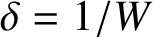 $\delta =1/W$
in (7-11), the inequality (7-5) follows with the choice
$\delta =1/W$
in (7-11), the inequality (7-5) follows with the choice
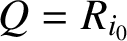 $Q=R_{i_{0}}$
.
$Q=R_{i_{0}}$
.
We next take advantage of the special direction vector
 $\mathbf {v}_{1}=(1,\alpha _{k},\alpha ^{2}_{k})$
, where
$\mathbf {v}_{1}=(1,\alpha _{k},\alpha ^{2}_{k})$
, where
 $\alpha _{k}$
is a cubic algebraic number given by (2-1) and (2-2). We apply some general results from Diophantine approximation, summarized in the next two lemmas. We use the standard notation
$\alpha _{k}$
is a cubic algebraic number given by (2-1) and (2-2). We apply some general results from Diophantine approximation, summarized in the next two lemmas. We use the standard notation
 $\Vert x\Vert $
to denote the distance of a real number x from the nearest integer.
$\Vert x\Vert $
to denote the distance of a real number x from the nearest integer.
The first lemma concerns badly approximable linear forms; see [Reference Schmidt10, Ch. II and Theorem 4A].
Lemma 7.2. Let
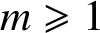 $m\geqslant 1$
be an integer, and let
$m\geqslant 1$
be an integer, and let
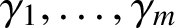 $\gamma _{1},\ldots ,\gamma _{m}$
be any m numbers in a real algebraic number field of degree
$\gamma _{1},\ldots ,\gamma _{m}$
be any m numbers in a real algebraic number field of degree
 $m+1$
such that
$m+1$
such that
 $1,\gamma _{1},\ldots ,\gamma _{m}$
are linearly independent over the rationals. Write
$1,\gamma _{1},\ldots ,\gamma _{m}$
are linearly independent over the rationals. Write
 $\mathbf {v}=(1,\gamma _{1},\ldots ,\gamma _{m})\in \mathbb {R}^{m+1}$
. Then there exists a constant
$\mathbf {v}=(1,\gamma _{1},\ldots ,\gamma _{m})\in \mathbb {R}^{m+1}$
. Then there exists a constant
 $C>0$
, depending at most on m and
$C>0$
, depending at most on m and
 $\gamma _{1},\ldots ,\gamma _{m}$
, such that
$\gamma _{1},\ldots ,\gamma _{m}$
, such that
 $$ \begin{align} \bigg\|\sum_{i=1}^{m}n_{i}\gamma_{i}\bigg\|\geqslant\frac{C}{(\max_{1\leqslant i\leqslant m}\vert n_{i}\vert)^{m}} \end{align} $$
for every
 $\mathbf {n}=(n_{1},\ldots ,n_{m})\in \mathbb {Z}^{m}$
with
$\mathbf {n}=(n_{1},\ldots ,n_{m})\in \mathbb {Z}^{m}$
with
 $\mathbf {n}\ne \mathbf {0}$
.
$\mathbf {n}\ne \mathbf {0}$
.
We comment that (7-12) follows relatively easily from the definition of the norm in an algebraic number field.
The second lemma is Mahler’s transference theorem in the relevant special case; see [Reference Mahler7] or [Reference Cassels2, Ch. 5 and Theorem 2].
Lemma 7.3. A necessary and sufficient condition that there exists a constant
 $C_{1}>0$
such that
$C_{1}>0$
such that
 $$ \begin{align*} \bigg\|\sum_{i=1}^mn_i\gamma_i\bigg\|\Big(\max_{1\leqslant i\leqslant m}\vert n_i\vert\Big)^m\geqslant C_1 \end{align*} $$
for every
 $\mathbf {n}=(n_{1},\ldots ,n_{m})\in \mathbb {Z}^{m}$
with
$\mathbf {n}=(n_{1},\ldots ,n_{m})\in \mathbb {Z}^{m}$
with
 $\mathbf {n}\ne \mathbf {0}$
, is that there exists another constant
$\mathbf {n}\ne \mathbf {0}$
, is that there exists another constant
 $C_{2}>0$
such that
$C_{2}>0$
such that
 $$ \begin{align*} \Big(\max_{1\leqslant j\leqslant m}\| n\gamma_j\|\Big)^{m} \vert n\vert\geqslant C_2 \end{align*} $$
for every
 $n\in \mathbb {Z}$
with
$n\in \mathbb {Z}$
with
 $n\ne 0$
.
$n\ne 0$
.
Let
 $\gamma _{1}=\alpha _{k}$
and
$\gamma _{1}=\alpha _{k}$
and
 $\gamma _{2}=\alpha _{k}^{2}$
. It follows from Lemma 7.2 that there exists a constant
$\gamma _{2}=\alpha _{k}^{2}$
. It follows from Lemma 7.2 that there exists a constant
 $C=C(\alpha _{k})>0$
, depending only on
$C=C(\alpha _{k})>0$
, depending only on
 $\alpha _{k}$
, such that
$\alpha _{k}$
, such that
 $$ \begin{align*} \| n_1\alpha_k+n_2\alpha_k^2\|\geqslant\frac{C}{(\max\{\vert n_1\vert, \vert n_2\vert\})^2} \end{align*} $$
for every
 $\mathbf {n}=(n_{1},n_{2})\in \mathbb {Z}^{2}$
with
$\mathbf {n}=(n_{1},n_{2})\in \mathbb {Z}^{2}$
with
 $\mathbf {n}\ne \mathbf {0}$
. It then follows from Lemma 7.3 that there exists another constant
$\mathbf {n}\ne \mathbf {0}$
. It then follows from Lemma 7.3 that there exists another constant
 $C^{\prime }=C^{\prime }(\alpha _{k})>0$
, depending only on
$C^{\prime }=C^{\prime }(\alpha _{k})>0$
, depending only on
 $\alpha _{k}$
, such that
$\alpha _{k}$
, such that
 $$ \begin{align} (\max\{\|n\alpha_{k}\|,\|n\alpha_{k}^{2}\|\})^{2}\vert n\vert\geqslant C^{\prime} \end{align} $$
for every
 $n\in \mathbb {Z}$
with
$n\in \mathbb {Z}$
with
 $n\ne 0$
.
$n\ne 0$
.
Consider the two-dimensional vector
 $\mathbf {w}_{1}=(\alpha _{k},\alpha ^{2}_{k})$
. Note that the transformation
$\mathbf {w}_{1}=(\alpha _{k},\alpha ^{2}_{k})$
. Note that the transformation
 $T=T_{\mathbf {v}_{1}}:X_{0}\to X_{0}$
modulo one reduces to the
$T=T_{\mathbf {v}_{1}}:X_{0}\to X_{0}$
modulo one reduces to the
 $\mathbf {w}_{1}$
-shift
$\mathbf {w}_{1}$
-shift
 $$ \begin{align} \mathbf{x}\to\mathbf{x}+\mathbf{w}_{1}\bmod{[0,1)^{2}} \end{align} $$
on the flat unit torus
 $[0,1)^{2}$
.
$[0,1)^{2}$
.
Applying (7-4) in the case when B is the nonempty open square
 $Q=Q(W)$
, we deduce that for
$Q=Q(W)$
, we deduce that for
 $\nu $
-almost every
$\nu $
-almost every
 $z\in X_{0}$
, we have
$z\in X_{0}$
, we have
 $$ \begin{align} \lim_{m\to\infty}\frac{1}{m}\sum_{j=0}^{m-1}\chi_{Q}(T^{j}z)=\nu(Q), \end{align} $$
where
 $\chi _{Q}$
is the characteristic function of Q. Let
$\chi _{Q}$
is the characteristic function of Q. Let
 $z=z_{0}$
in
$z=z_{0}$
in
 $X_{0}$
satisfy (7-15). Then there exists a threshold
$X_{0}$
satisfy (7-15). Then there exists a threshold
 $m_{0}$
such that for every
$m_{0}$
such that for every
 $m\geqslant m_{0}$
, we have
$m\geqslant m_{0}$
, we have
 $$ \begin{align} \frac{1}{m}\sum_{j=0}^{m-1}\chi_{Q}(T^{j}z_{0})=\frac{\nu(Q)}{2}. \end{align} $$
Choosing m sufficiently large, we can guarantee that
 $1/\sqrt {m}$
is much smaller than the side length of the square Q. We divide Q into small congruent subsquares
$1/\sqrt {m}$
is much smaller than the side length of the square Q. We divide Q into small congruent subsquares
 $R_{i}$
,
$R_{i}$
,
 $i\in I$
, of side length
$i\in I$
, of side length
 $1/r$
, where
$1/r$
, where
 $m=C^{\prime }r^{2}$
and
$m=C^{\prime }r^{2}$
and
 $C^{\prime }>0$
is the constant in (7-13). Thus, if we ignore, for notational simplicity, those small squares
$C^{\prime }>0$
is the constant in (7-13). Thus, if we ignore, for notational simplicity, those small squares
 $R_{i}$
that intersect the boundary of Q, then with negligible error if m is sufficiently large, we have
$R_{i}$
that intersect the boundary of Q, then with negligible error if m is sufficiently large, we have

We claim that
 $$ \begin{align} T^{-j_{1}}R_{i}\cap T^{-j_{2}}R_{i}=\emptyset, \quad i\in I,\ 0\leqslant j_{1}<j_{2}\leqslant m-1. \end{align} $$
Suppose, to the contrary, that there exist
 $i\in I$
and integers
$i\in I$
and integers
 $0\leqslant j_{1}<j_{2}\leqslant m-1$
such that
$0\leqslant j_{1}<j_{2}\leqslant m-1$
such that
 $T^{-j_{1}}R_{i}$
intersects
$T^{-j_{1}}R_{i}$
intersects
 $T^{-j_{2}}R_{i}$
. Let
$T^{-j_{2}}R_{i}$
. Let
 $$ \begin{align*} \mathbf{u}\in T^{-j_1}R_i\cap T^{-j_2}R_i. \end{align*} $$
Then both
 $T^{j_{1}}\mathbf {u}$
and
$T^{j_{1}}\mathbf {u}$
and
 $T^{j_{2}}\mathbf {u}$
are elements of the same small square
$T^{j_{2}}\mathbf {u}$
are elements of the same small square
 $R_{i}$
of side length
$R_{i}$
of side length
 $1/r$
. Applying the modulo one reduction in (7-14), we see that
$1/r$
. Applying the modulo one reduction in (7-14), we see that
 $\mathbf {u}+j_{1}\mathbf {w}_{1}$
and
$\mathbf {u}+j_{1}\mathbf {w}_{1}$
and
 $\mathbf {u}+j_{2}\mathbf {w}_{1}$
are
$\mathbf {u}+j_{2}\mathbf {w}_{1}$
are
 $1/r$
-close to each other on the flat torus
$1/r$
-close to each other on the flat torus
 $[0,1)^{2}$
, and so
$[0,1)^{2}$
, and so
 $(j_{2}-j_{1})\mathbf {w}_{1}$
and
$(j_{2}-j_{1})\mathbf {w}_{1}$
and
 $\mathbf {0}=(0,0)$
are
$\mathbf {0}=(0,0)$
are
 $1/r$
-close to each other on the flat torus
$1/r$
-close to each other on the flat torus
 $[0,1)^{2}$
. Thus,
$[0,1)^{2}$
. Thus,
 $$ \begin{align} (\max\{\|(j_{2}-j_{1})\alpha_{k}\|,\|(j_{2}-j_{1})\alpha_{k}^{2}\|\})^{2}\leqslant\frac{1}{r^{2}}=\frac{C^{\prime}}{m}. \end{align} $$
On the other hand, applying (7-13) with
 $n=j_{2}-j_{1}$
, we obtain
$n=j_{2}-j_{1}$
, we obtain
 $$ \begin{align*} (\max\{\|(j_2-j_1)\alpha_k\|,\|(j_2-j_1)\alpha_k^2\|\})^2\geqslant\frac{C'}{j_2-j_1}>\frac{C'}{m}, \end{align*} $$
contradicting (7-19). This establishes (7-18).
We are ready to complete the proof of Theorem 6.3. Combining (7-16) and (7-17), we have, for every
 $m\geqslant m_{0}$
,
$m\geqslant m_{0}$
,
 $$ \begin{align} \frac{\nu(Q)m}{2} \leqslant\sum_{j=0}^{m-1}\chi_{Q}(T^{j}z_{0}) =\sum_{i\in I}\sum_{j=0}^{m-1}\chi_{R_{i}}(T^{j}z_{0}) \leqslant\vert I\vert, \end{align} $$
where the last inequality is a consequence of (7-18).
Combining (7-5), (7-17), (7-19) and (7-20), we conclude that

But this is absurd, since
 $2/C^{\prime }$
is a constant depending only on
$2/C^{\prime }$
is a constant depending only on
 $\alpha _{k}$
, and W can be arbitrarily large. This completes the proof of Theorem 6.3. □
$\alpha _{k}$
, and W can be arbitrarily large. This completes the proof of Theorem 6.3. □
Finally, we discuss how we can extend Theorems 6.1–6.4 concerning the L-solid to any polycube
 $3$
-manifold with one-direction geodesic flow, and establish Theorem 1.1.
$3$
-manifold with one-direction geodesic flow, and establish Theorem 1.1.
Let
 $\mathcal {P}$
be an arbitrary polycube
$\mathcal {P}$
be an arbitrary polycube
 $3$
-manifold. Our task is to extend the proof of Theorem 6.1 given in the special case of the L-solid with street-LCM equal to
$3$
-manifold. Our task is to extend the proof of Theorem 6.1 given in the special case of the L-solid with street-LCM equal to
 $2$
to the case of
$2$
to the case of
 $\mathcal {P}$
with one-direction geodesic flow. We know that
$\mathcal {P}$
with one-direction geodesic flow. We know that
 $\mathcal {P}$
has X-streets, Y-streets and Z-streets, and that the street-LCM of
$\mathcal {P}$
has X-streets, Y-streets and Z-streets, and that the street-LCM of
 $\mathcal {P}$
is the least common multiple of the lengths of all the streets.
$\mathcal {P}$
is the least common multiple of the lengths of all the streets.
We can clearly adapt Sections 3–5, as the discussion in these sections does not use any special property of the L-solid that is not present in an arbitrary polycube
 $3$
-manifold. For notational convenience, and for easy visualization, we chose to work earlier with the simplest concrete special case of the L-solid.
$3$
-manifold. For notational convenience, and for easy visualization, we chose to work earlier with the simplest concrete special case of the L-solid.
To generalize the argument in Section 6, we need a time-quantitative density result for any polycube
 $3$
-manifold. The following result is [Reference Beck, Chen and Yang1, Theorem 6.4.2], and is a straightforward generalization of time-quantitative density A in Section 2.
$3$
-manifold. The following result is [Reference Beck, Chen and Yang1, Theorem 6.4.2], and is a straightforward generalization of time-quantitative density A in Section 2.
Let
 $\eta>0$
be an arbitrarily small but fixed positive number. We say that a half-infinite geodesic
$\eta>0$
be an arbitrarily small but fixed positive number. We say that a half-infinite geodesic
 $\mathcal {L}$
in
$\mathcal {L}$
in
 $\mathcal {P}$
is
$\mathcal {P}$
is
 $\eta $
-nearly superdense if there exists an effectively computable explicit threshold
$\eta $
-nearly superdense if there exists an effectively computable explicit threshold
 $N_{0}(\mathcal {P};\eta )$
such that, for every integer
$N_{0}(\mathcal {P};\eta )$
such that, for every integer
 $n\geqslant N_{0}(\mathcal {P};\eta )$
, the initial segment of
$n\geqslant N_{0}(\mathcal {P};\eta )$
, the initial segment of
 $\mathcal {L}$
with length
$\mathcal {L}$
with length
 $n^{2+\eta }$
intersects every axis-parallel cube of side length
$n^{2+\eta }$
intersects every axis-parallel cube of side length
 $1/n$
in
$1/n$
in
 $\mathcal {P}$
.
$\mathcal {P}$
.
Lemma 7.4. Let
 $\mathcal {P}$
be an arbitrary polycube
$\mathcal {P}$
be an arbitrary polycube
 $3$
-manifold, and let
$3$
-manifold, and let
 $h=h(\mathcal {P})$
denote the street-LCM of
$h=h(\mathcal {P})$
denote the street-LCM of
 $\mathcal {P}$
. Let
$\mathcal {P}$
. Let
 $\eta>0$
be fixed. There exists a threshold
$\eta>0$
be fixed. There exists a threshold
 $K_{0}(\mathcal {P};\eta )$
such that for every integer
$K_{0}(\mathcal {P};\eta )$
such that for every integer
 $k\geqslant K_{0}(\mathcal {P};\eta )$
, any half-infinite geodesic in
$k\geqslant K_{0}(\mathcal {P};\eta )$
, any half-infinite geodesic in
 $\mathcal {P}$
with direction given by one of the vectors in (1-2), where
$\mathcal {P}$
with direction given by one of the vectors in (1-2), where
 $\alpha _{k}$
is a root of the cubic equation
$\alpha _{k}$
is a root of the cubic equation
 $x^{3}+hkx-1=0$
in the interval
$x^{3}+hkx-1=0$
in the interval
 $$ \begin{align*} \frac{1}{hk+1}<\alpha_k<\frac{1}{hk}, \end{align*} $$
is
 $\eta $
-nearly superdense in
$\eta $
-nearly superdense in
 $\mathcal {P}$
.
$\mathcal {P}$
.
Using this density result, it is fairly straightforward to generalize the argument in Section 6 to establish an analog of Theorem 6.1 for any polycube
 $3$
-manifold. Finally, repeating the arguments in the derivation of Theorems 6.2–6.4 from Theorem 6.1, we can complete the proof of Theorem 1.1.
$3$
-manifold. Finally, repeating the arguments in the derivation of Theorems 6.2–6.4 from Theorem 6.1, we can complete the proof of Theorem 1.1.


