1. INTRODUCTION
Inertial Navigation Systems (INSs) have high data update rates, low noise, and provide high accuracy over a short period of time. However, INS errors accumulate over time and are integrated into progressively larger errors. In contrast, errors in Global Navigation Satellite Systems (GNSSs) are independent of time. In addition, GNSSs can work around the clock and provide high-precision worldwide navigational information. However, the update rate of the information is relatively low (Hu et al., Reference Hu, Liu, Gao and Yang2015). After processing the information using filter fusion methods, a combined GNSS/INS system can provide complementary advantages leading to more accurate navigation results. According to different degrees of coupling there are two main modes: loosely coupled mode and tightly coupled mode. Because the loosely coupled mode is the more mature, the following discussion is based on a loosely coupled GNSS/INS system.
For linear systems, whose process noise and measurement noise are white noise sequences, the result of the Kalman Filter (KF) is optimal in the unbiased, consistent, and progressively effective sense (Li et al., Reference Li, Jin and Chang2015). GNSS signals are easily disturbed by the external environment causing the GNSS to produce large observation outliers of two typical types, single or continuous. The former can be caused by multi-path effect (Yedukondalu et al., Reference Yedukondalu, Sarma and Ashwani2013). For example, a small puddle of water in the road reflects the signal and the reflected signal transiently disturbs the original one. A series of continuous outliers may come from the sustained shelter of long tunnels, tall buildings or canyons. There may also be sustained multi-path effects caused by a long reflector. The density of observations would then perform as a distribution with a long tail (Liu et al., Reference Liu, Sun and Chen2012). Moreover, the observation noises will no longer follow a Gaussian distribution, nor will they follow the basic assumptions of the KF. As a result, filtering performance degrades, and the demands cannot be satisfied.
Based on the KF, the particle filter, self-adapting filter, and H∞ filter with better robust performance have been designed (Miao et al., Reference Miao, Zhou, Tian and Cui2016). The particle filter can be applied to nonlinear systems; however, its computation is complex with poor real-time performance. It is seldom used in the field of integrated navigation. The self-adapting filter includes the Least Mean Squares (LMS) and Recursive Least Squares (RLS) methods; however, its tracking performance is poor. The H∞ filter analyses error information according to the index of the filtering performance. Its energy is the lowest; however, the average estimation precision is discarded to obtain a more robust performance (Godha, Reference Godha2006). To deal with these drawbacks, an improved method is proposed so as to improve the robust performance of an integrated navigation system.
The remainder of this paper is organised as follows. In Section 2, a model for a loosely coupled GNSS/INS integrated navigation system is established. In Section 3, the standard KF is described as the basis of this method, including the steps and equations. In Section 4, the method for detecting and suppressing the outliers is proposed based on the above sections. This method uses the χ2-test algorithm of the innovation vector to detect the outliers and construct a scale factor according to the innovation vector in order to adjust the filter gain dynamically. In this way, the influence of the observation outliers is reduced. In Section 5, simulation results demonstrate that the proposed method is capable of detecting and suppressing the outliers of a GNSS/INS integrated navigation system. In Section 6, real road tests show that the proposed methods can effectively improve the navigation system.
2. MODEL OF THE INS/GNSS INTEGRATED NAVIGATION SYSTEM
The principle of a GNSS/INS integration is as follows. The estimated values of position and velocity are obtained respectively by GNSS and INS. The corresponding differences can then be obtained, and they are inputted into a filter, such as a KF. The outputs of the filter, which are called estimated errors, are fed back to the INS and used to correct the INS outputs. In this way, the INS outputs become more accurate.
Using the error equation of an INS, the observation equation and state equation of the integrated navigation system are established, and the state-space method is used to express them (Woodman, Reference Woodman2007). The navigation coordinate frame used in this study is the East-North-Up (ENU) coordinate frame. The origin point O is located at the centroid of the carrier. The x-axis and y-axis represent the eastward and northward along E and N, respectively, and the z-axis points to the sky.
2.1. INS error equation
Along with the error equations of attitude angle, velocity and position and the error model of the inertial device, we obtain the INS error equation. Omitting the derivation and using the state-space method, the equation is given by:
 $$\dot{x} = Fx + W$$
where x is the state parameters in the form of a 9×1 dimension matrix including attitude angle errors in three directions Φx, Φy and Φz, errors of latitude, longitude and altitude δ φ, δ λ and δA and velocity errors in three directions δ v x, δ v y and δ v z. F is the 9×9 dimension coefficient matrix which can convert x to  $\dot{x}$ and W is the random error matrix of the inertial device.
2.2. The GNSS/INS state and observation equations
GNSS error is regarded as observation noise in GNSS/INS integrated navigation systems (Angrisano et al., Reference Angrisano, Petovello and Pagliano2010). The state equation of the integrated system is the same as Equation (1) for the INS.
The time constant of position estimation is far greater than that of velocity estimation, so position is observed once after velocity has been observed several times and this action is repeated (Luo et al., Reference Luo, Ma, Yuan and Yue2012). By alternately observing the position and velocity, the observation equation of the integrated navigation system can be obtained from the difference of the observed value of the INS and the GNSS:
 $$y = Hx = V$$
where H is the local position and velocity parameter matrix and V is the random white noise matrix of the position and velocity observations of the GNSS.
3. STANDARD KALMAN FILTERING ALGORITHM
Due to the uncertainty of the noise in practical applications (Chang, Reference Chang2014), the state and observation equations are combined which aims to predict the next-moment state vector and is then corrected in the Kalman filtering algorithm (Koch, Reference Koch2014). A set of equations for the optimal state estimation can be obtained.
Assuming there is a dynamic system model:
 $$\lcub \eqalign{& X_k = \Phi_{k|k-1}X_{k-1}+\Gamma_{k-1}W_{k-1} \cr & Y_k = H_kX_k + V_k } $$
where W k and V k are white Gaussian noise and are not related to each other. The mean and variance of the initial vector X 0 are known and W k, V k and X 0 are not related.
Given below are the equations of Kalman filtering:
1. One step prediction of the state equation
(4) $$\hat{X}_{k|k-1} = \Phi_{k|k-1}\hat{X}_{k-1}$$
2. One step prediction of the mean-square error equation
(5)$$\eqalign{P_{k|k-1}&= \Phi_{k|k-1}P_{k-1}\Phi^T_{k|k-1}\cr &\quad + \Gamma_{k-1}Q_{k-1}\Gamma^T_{k-1}}$$3. Innovation vector
(6)$$i_k = Y_k - H_k \hat{X}_{k-1}$$4. Equation of filter gain
(7)$$K_{k|k-1} = P_{k|k-1}H^T_k (H_kP_{k|k-1}H^T_k + R_k)^{-1}$$5. Equation of state estimation
(8)$$\hat{X}_k = \hat{X}_{k|k-1} + K_k i_k$$6. Equation of estimated mean square error
(9)$$\eqalign{P_k &= (I-K_kH_k)P_{k|k-1}(I-K_kH_k)^T \cr &\quad + K_k R_k K^T_k}$$


where:
- $\hat{X}_{k \vert k-1}$ is the predicted state vector calculated from the optimal state estimation $\hat{X}_{k-1}$ at k-1,
Φk|k−1 is the state transition matrix from moment k-1 to moment k,
P k|k−1 is the predicted error variance matrix from moment k-1 to moment k,
Γk−1 and Q k−1 are the interference matrix and interference-variance matrix, respectively,
i k is the innovation vector, which contains the new information provided by the newest observations,
H k is the parameter matrix of observation at moment k and K k is the gain matrix,
R k is the observation noise covariance matrix and is a symmetrical positive definite matrix,
- $\hat{X}_{k}$ is the optimal estimate state vector and is estimated from the present value and the predicted state vector and
P k is the estimated mean-square error matrix at moment k.


4. DETECTION AND SUPPRESSION OF OBSERVATION OUTLIERS
An INS is normally isolated from the outside environment in some way. Therefore, outliers seldom appear over a short time span (Quan et al., Reference Quan, Liu, Gong and Fang2011). In contrast, a GNSS receives signals from the environment and outliers may appear suddenly at any time. GNSS is the main source of outliers.
4.1. χ2-test observation outliers algorithm
The new observation is introduced to the system when the innovation vector i k is solved using the Kalman filtering equations shown above. Consequently, the outliers can be detected according to the feature of innovation vector i k.
According to the definition, the innovation vector i k is a Gaussian white noise sequence with a mean value of zero. It obeys a normal distribution:
 $$i_k \sim N(0, H_k P_{k|k-1} H^T_k + R_k)$$
The value of i k will change when there are observation outliers in the GNSS as the subsystem of the integrated navigation system. Since i k is not a Gaussian white noise sequence any more, the detection of outliers can be transformed into a hypothesis testing problem due to the change in the statistical characteristics of i k. The matrix of the innovation vector, I is constructed and obeys the χ2 distribution:
 $$I = i^T_k (H_k P_{k|k-1} H^T_k + R_k)^{-1}i_k$$
where H k is the parameter matrix of the observation at moment k and P k|k−1 is the variance matrix of prediction error from moment k-1 to moment k.
A null hypothesis is proposed that is H 0: I ~ χ 2 (t). The following are the detection steps:
(1) A small value α is chosen as the level of significance. The α represents the threshold of probability. The smaller it is, the more accurate the detection. Its action mechanism is in step (3).
(2) The corresponding superior position point
$\chi^{2}_{\alpha,t}$ of α is obtained by look-up table and is known as the threshold value. It is the critical condition that judges whether the null hypothesis H 0 is correct.(3) Obtain the probability p of equation
$I > \chi^{2}_{\alpha , t}$. If p<α, the null hypothesis H 0 is incorrect. If α is small, it is said the probability p of $I > \chi^{2}_{\alpha , t}$ is very small and H 0 is rejected which is to say it seldom happens when this situation occurs. Outlier detection can hence be concluded. In step (3), I and $\chi^{2}_{\alpha ,t}$ should be compared directly. If $I > \chi^{2}_{\alpha , t}$, there are outliers.


4.2. The observation outlier suppression method
The observation outliers can be discarded or reduced in weight after being detected. However, if the outliers are continuous in time, only the INS functions correctly and if an outlier is too large, a long time is needed to remove the influence of outliers. Considering these problems, the following method is adopted to tackle it. A scale factor is constructed referring to the innovation vector i k and then the filtering gain is adjusted dynamically by the scale factor to suppress the outliers.
According to Equation (8), when the observation values change, the innovation i k changes and the filtering gain matrix K k is unchanged. Then, the deviation of estimated result  $\hat{X}_{k}$ appears. Considering this, an adjustment of K k based on i k is used to reduce the influence of outliers on
  $\hat{X}_{k}$.
Normally, the innovation vector i k is a Gaussian white noise sequence. Moreover, the single innovation also follows the normal distribution with zero mean. I k satisfies the condition described below:
 $$I_k\sim \chi^2(1)$$
When an outlier is detected, the scale factor μ is constructed:
 $$\mu = {I_k \over \chi^2_{\alpha}}$$
When outliers appear, K k is expanded by the scale factor shown in Equation (13):
 $$\overline{K}_k = K_k /\mu$$
 By replacing K k with  $\overline{K}_{k}$ and filtering it again, the filtering result after the outliers being suppressed is obtained.
It is obvious that μ is greater than 1 from Equation (13). When the outliers appear, the filtering gain matrix is reduced correspondingly. Then the state estimated result is limited in a normal range by the reduced filtering gain matrix.
5. SIMULATION
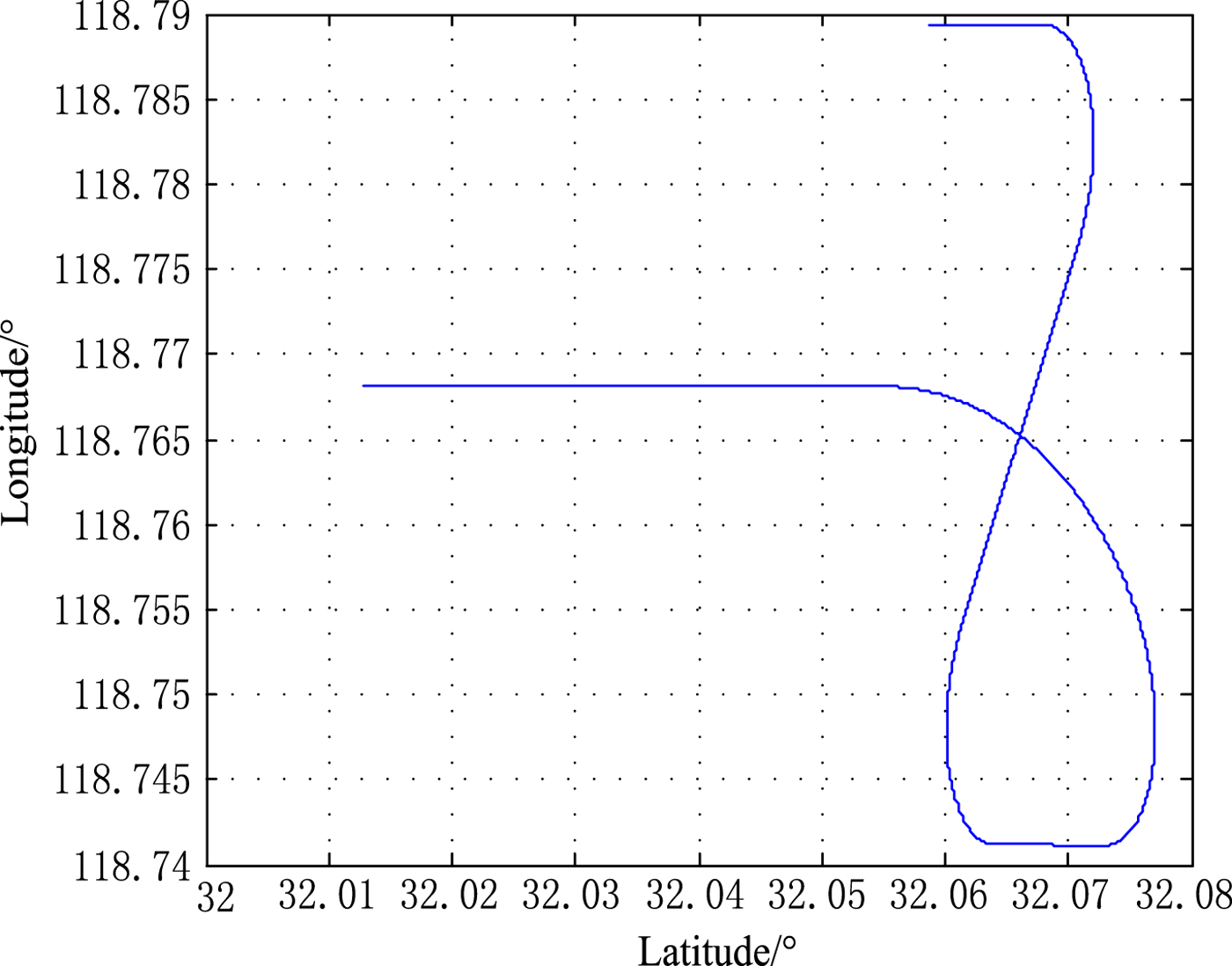
An integrated navigation system is simulated to verify the effectiveness of the proposed algorithm (Simon, Reference Simon2006). The parameters of the simulation are set as follows: the initial latitude, longitude, and height are 32·05862°, 118·78938° and 14 m, respectively. The root mean square value of the constant drift of the gyro's error is 0 · 1°/h. The root mean square value of the gyro's white noise is 0 · 1°/h. The constant zero offset of the accelerometer's error and the measured white noise are both 5 × 10⁻⁵g. The heading, roll and pitch angles are 30′′, 60′′ and 30′′, respectively. In the horizontal direction, the position deviation, random deviation, and velocity deviation are 10 m, 32 m and 0·5 m/s, respectively. The total time of the simulation is 990 s. The simulation trace is shown in Figure 1.

Figure 1. Trace of simulated path.
Now we compare the results with and without the outlier processing algorithm. There are three cases: no outlier, single outlier over a certain moment and continuous outliers at a certain period of time. The following is a comparison of different situations:
Case 1: There is no outlier. Here, the performances of the two filters are compared under normal conditions.
From Figures 2 to 4 and Table 1, we observe that the performance of the system before and after being processed by the adjusting method of filter gain is comparable. This shows that although the processing method is designed for outliers, the false detection probability of the normal value is very small, and under normal circumstances, the best filtering performance is achieved.
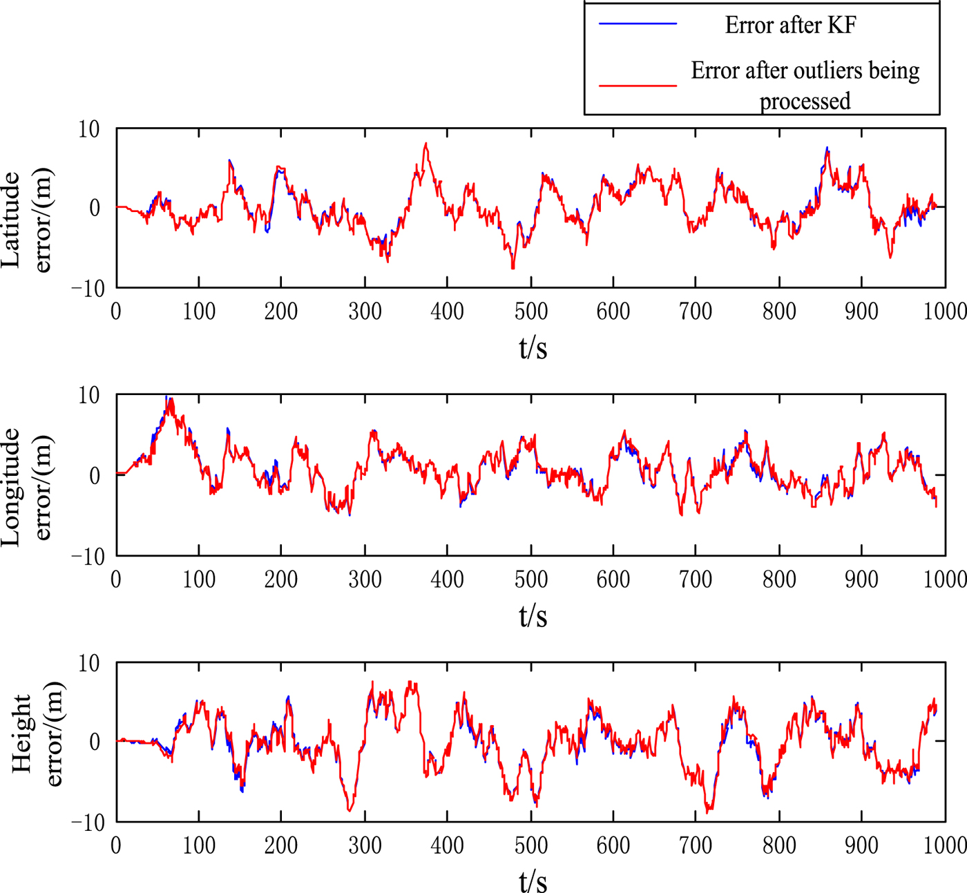
Figure 2. Position error contrast under normal condition.
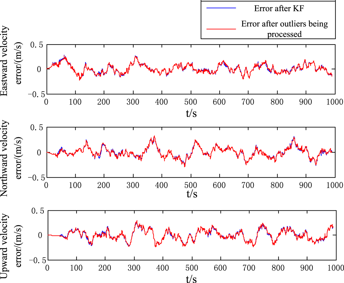
Figure 3. Velocity error contrast in normal conditions.
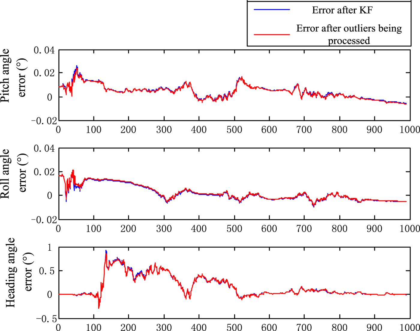
Figure 4. Attitude error contrast under normal conditions.
Table 1. Comparison of error RMS under different conditions.

Case 2: One outlier at a certain moment. From 100 s to 400 s, a 50 m latitude error is introduced every 100 s; from 600 s to 900 s, a 50 m longitude error is introduced every 100 s. The performance of the two filtering methods is then compared. We then replace the 50 m error with small errors which are 25 m and 10 m and do the same comparison to test the effectiveness of the method when errors are small. The significance level α when dealing with outliers is set as 0·01. In addition, the corresponding superior position point  $\chi_{\alpha}^{2}$ is set as 6·35, that is, the threshold value is 6·35.
From Figures 5 to 7 and Table 1, we observe that the standard KF is disturbed and the filtering results increase by three to four times when the single 50 m outlier is introduced. In addition, the influence exists for approximately 100 s after the outliers fade away. After being processed by the adjusting methods, the single outlier is detected and restrained. In the direction in which the error is introduced, the accuracy of filtering results of the position and velocity increase by 70%.
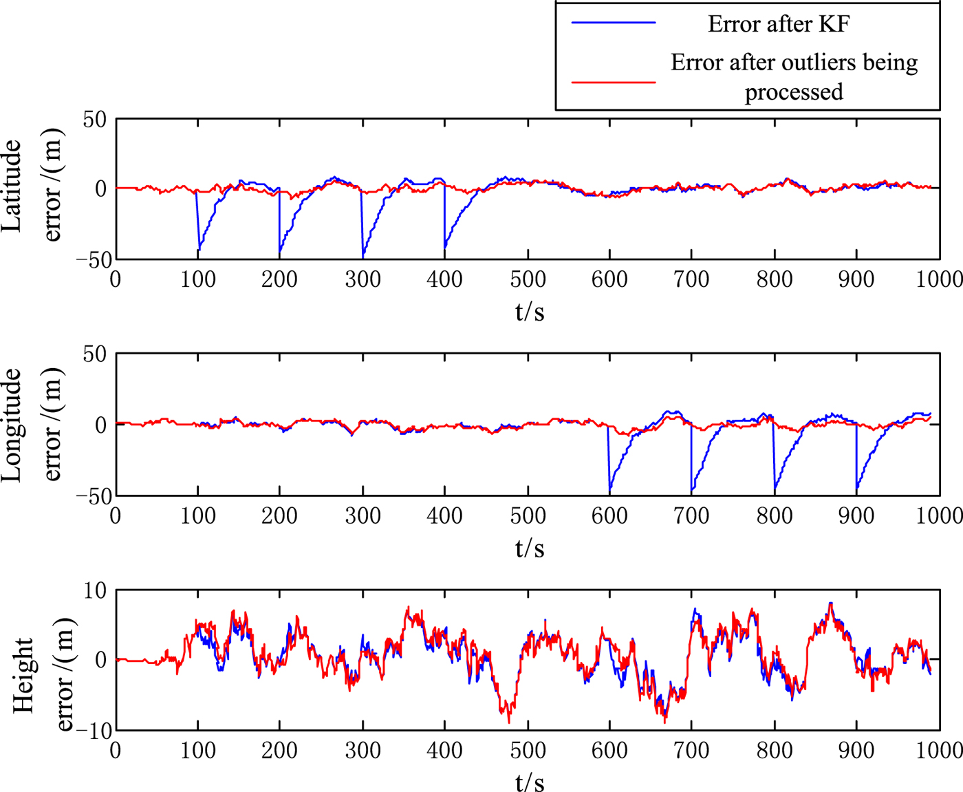
Figure 5. Position error contrast when a single 50 m outlier is introduced.
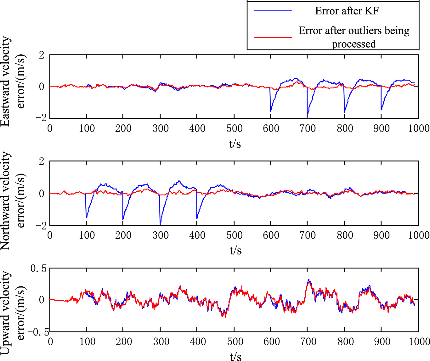
Figure 6. Velocity error contrast when a single 50 m outlier is introduced.

Figure 7. Attitude error contrast when a single 50 m outlier is introduced.
From Figures 8 to 9 and Table 1, we can see that when smaller errors, which are 25 m and 10 m, are introduced, the results of the KF improve. However, there are still outliers and 50 s unstable periods. However, the adjusting method worked. When the error is 25 m, the accuracy in position and velocity increases by about 50%. When the error is 10 m, the accuracy increases by 20% and the transient response is eliminated.
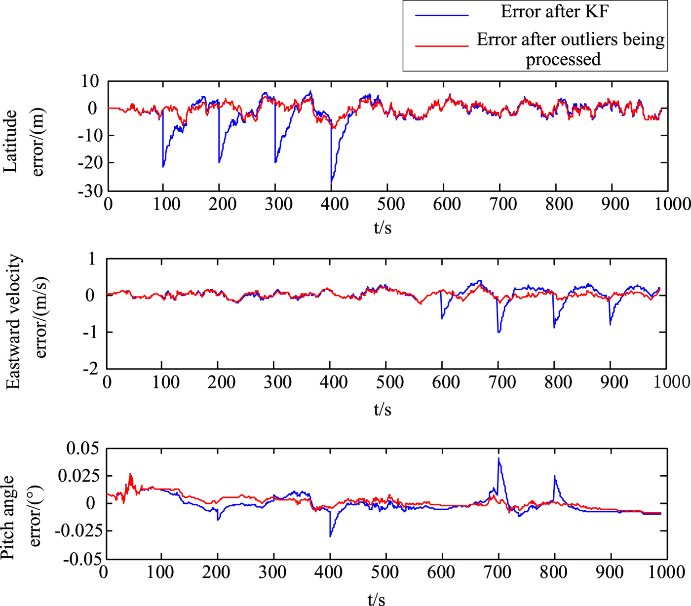
Figure 8. Error contrast when a single 25 m outlier is introduced (only part is shown).
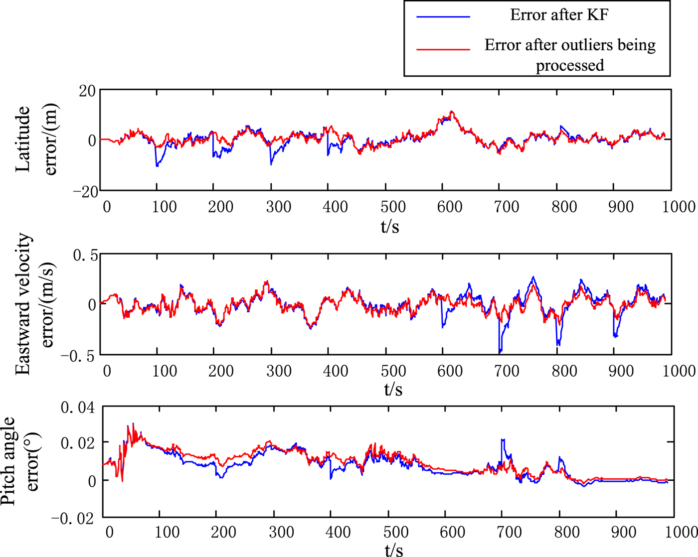
Figure 9. Error contrast when a single 10 m outlier is introduced (only part is shown).
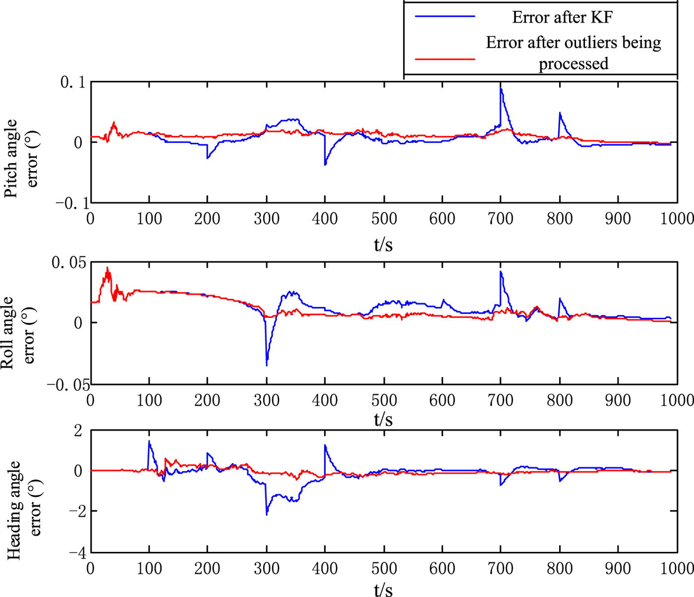
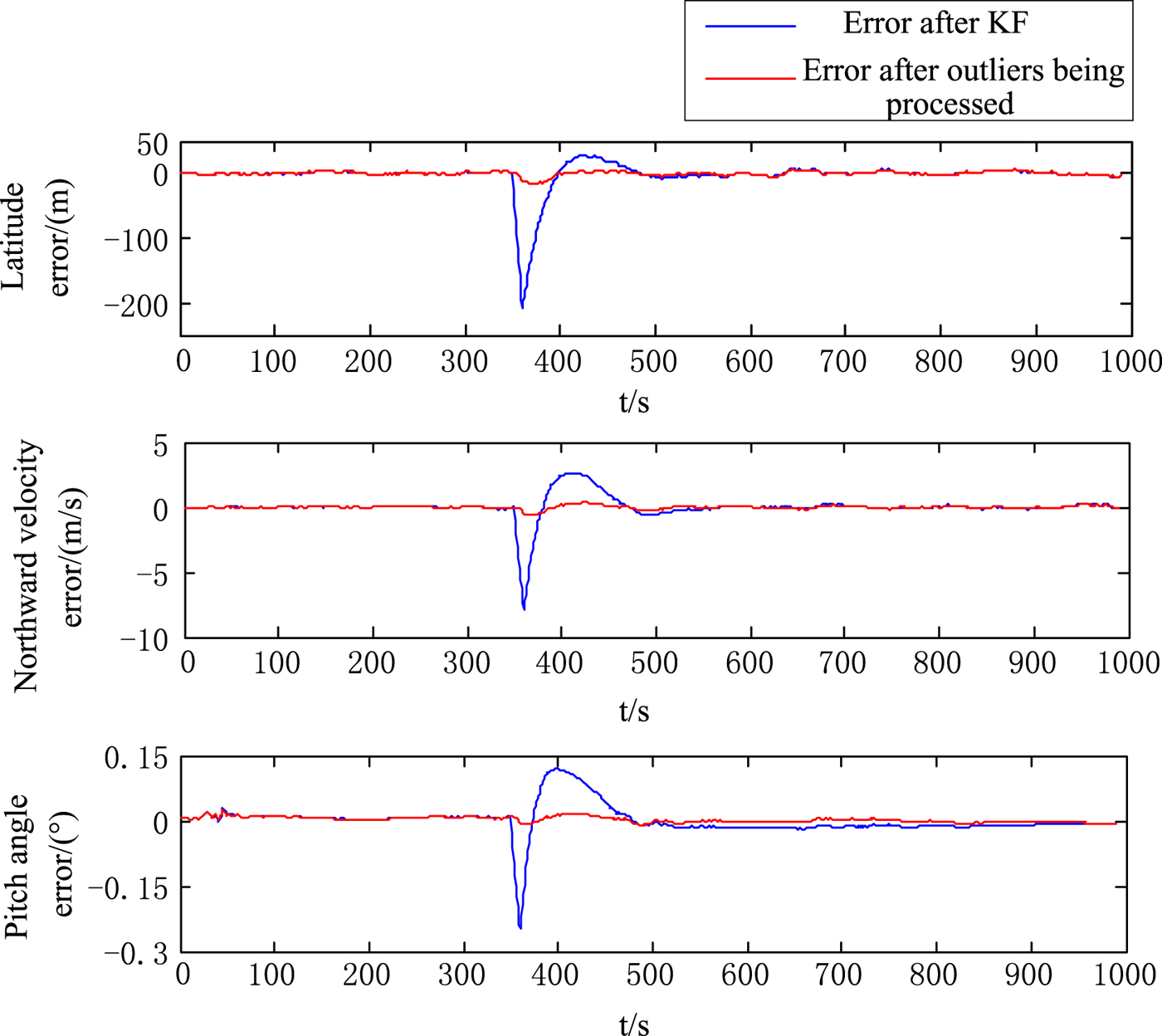
Case 3: Continuous outliers over a certain period. For simulating a problem over a certain period of time, a 50 m error is introduced in the latitude direction at 350–360 s. We then replace 50 m errors with small errors which are 25 m and 10 m and do the same comparison to test the effect of the method. To compare the result, we set the certain level α and the threshold to the same as that in case 2.
From Figures 10 to 12 and Table 1, we observe that the standard KF will be influenced greatly when 50 m continuous outliers are introduced every 10 s. The traditional filter struggles to process the outliers. After the outliers fade away, the filtering results will fluctuate violently around the time of 400 s. After being processed by adjusting methods of filter gain, the results of the position, velocity and attitude angle accuracies have increased by more than 90%. There is only a 20 s light fluctuation after outliers fade away.
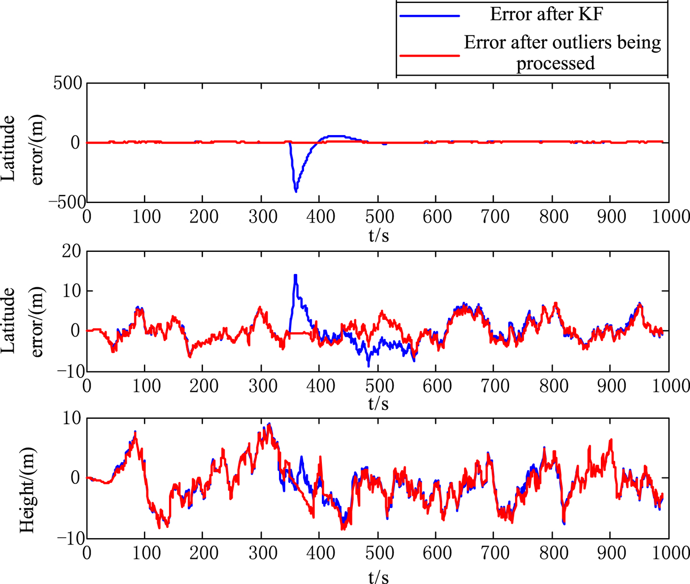
Figure 10. Position error contrast when 10 s 50 m outliers are introduced.
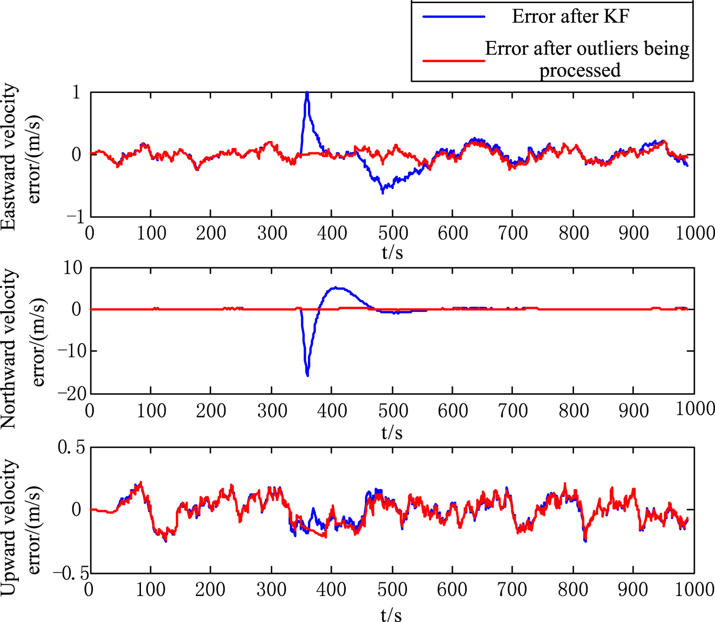
Figure 11. Velocity error contrast when 10 s 50 m outliers are introduced.

Figure 12. Attitude error contrast when 10 s 50 m outliers are introduced.
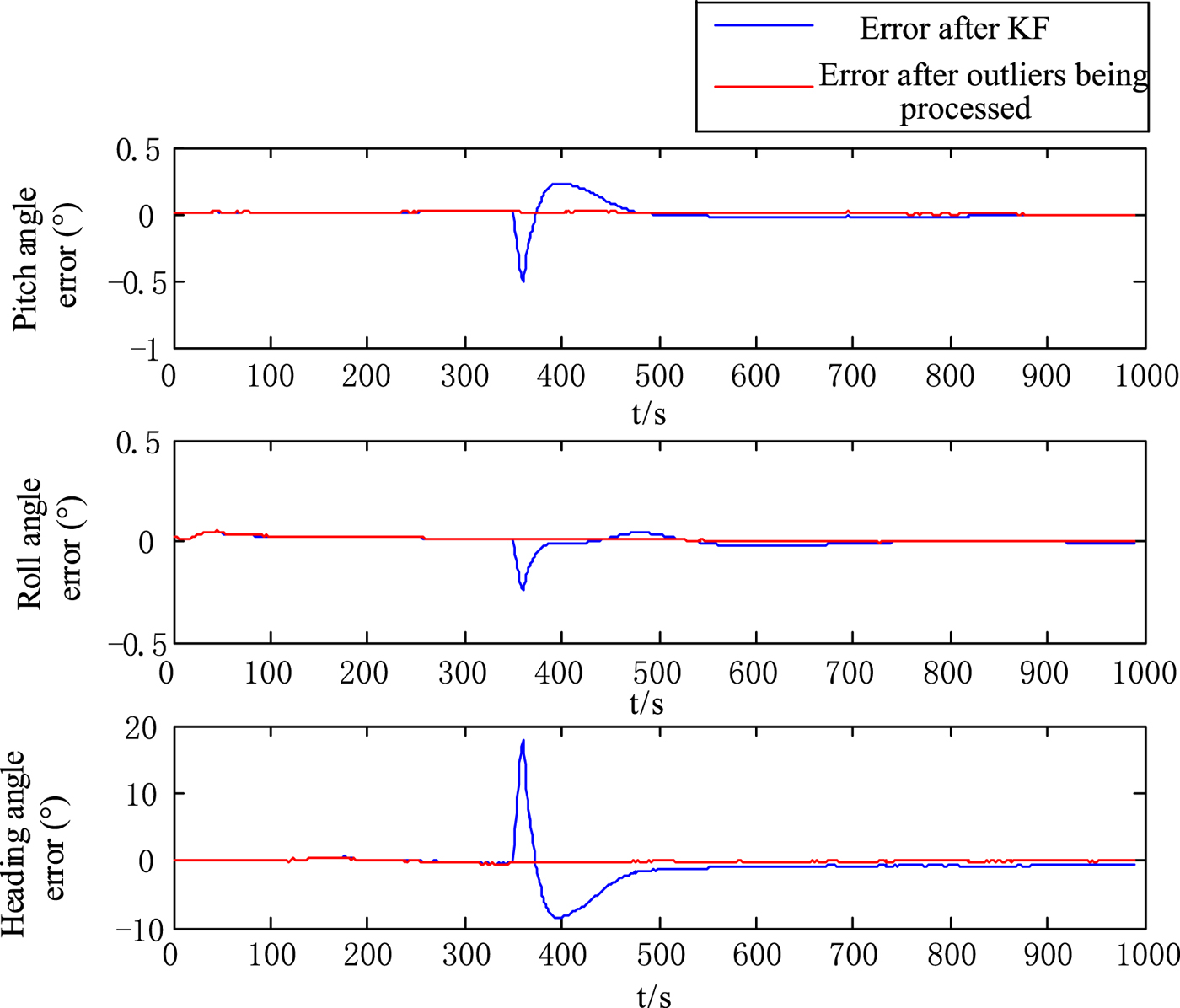
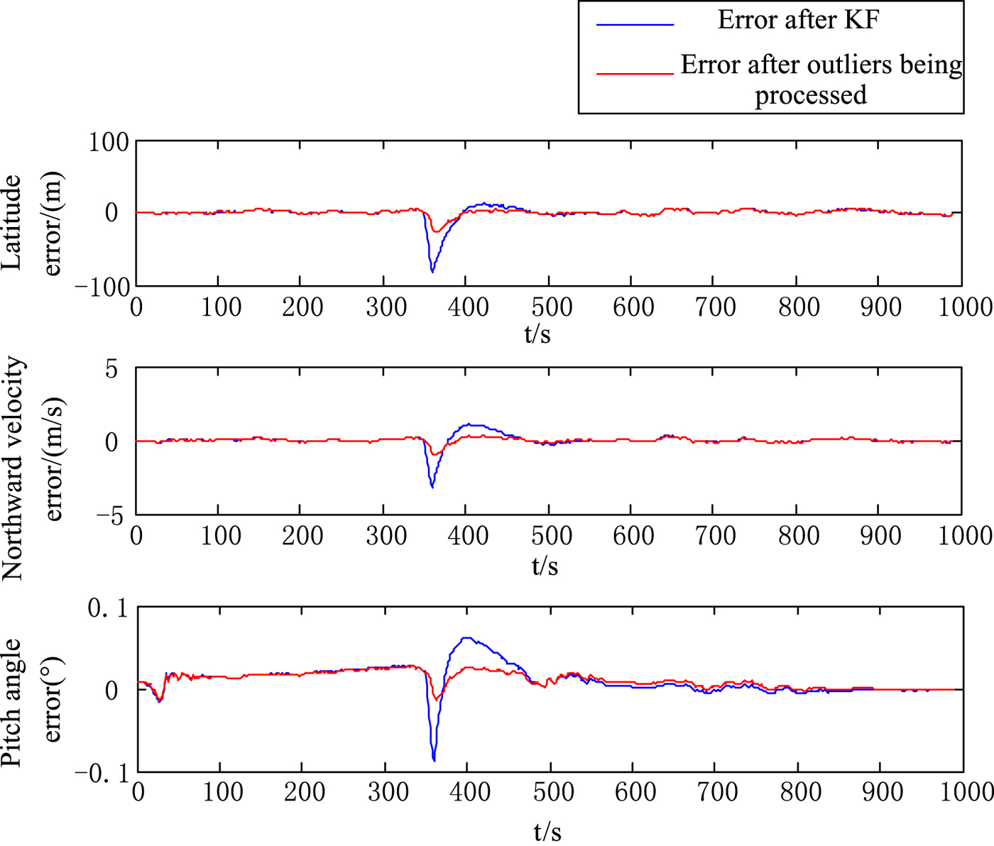
From Figures 13 to 14 and Table 1, when 25 m continuous outliers are introduced, the results of the KF will fluctuate sharply and there will be a 100 s unstable period. After being processed by the adjusting method, the accuracy of the results has been enhanced by 70% to 90%. When errors are 10 m, the accuracy increases by about 50%. Both the unstable time periods shrink to about 20 s.

Figure 13. Errors contrast when 10 s 25 m outliers are introduced.

Figure 14. Errors contrast when 10 s 10 m outliers are introduced.
6. EXPERIMENTS
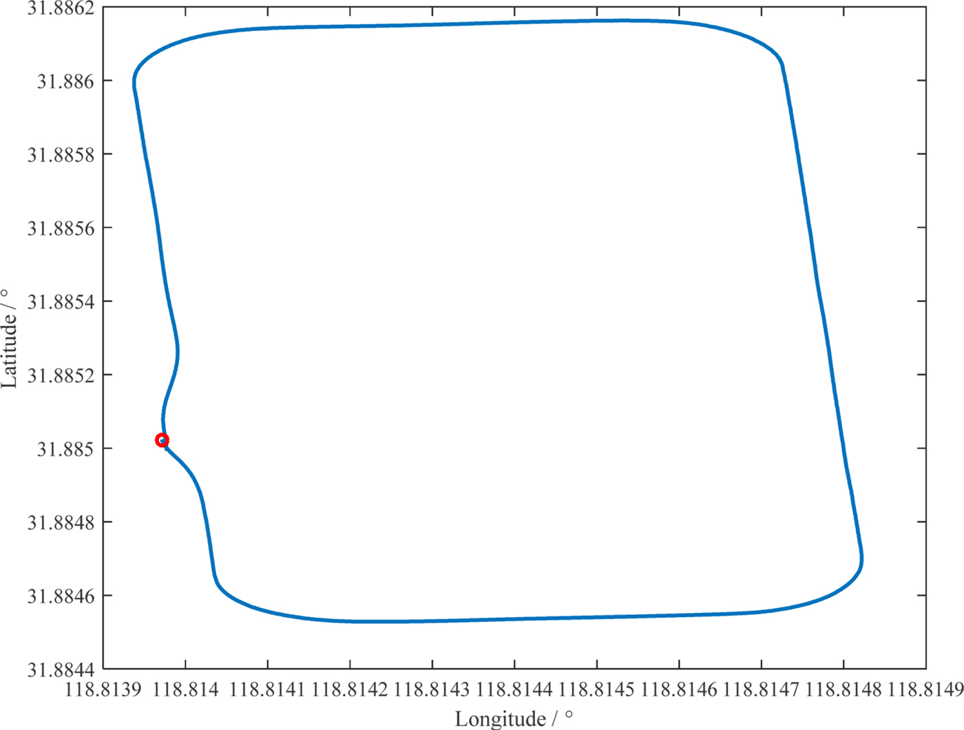
To further evaluate the performance of the proposed method, the experimental data provided by the vehicle in Figure 15 is treated as the navigation data. The experimental vehicle system includes a Micro-Electromechanical System (MEMS)-based IMU, GNSS receiver and navigation computer. The total time of the test was 243 s. Figure 16 shows the trajectory of the experimental vehicle.
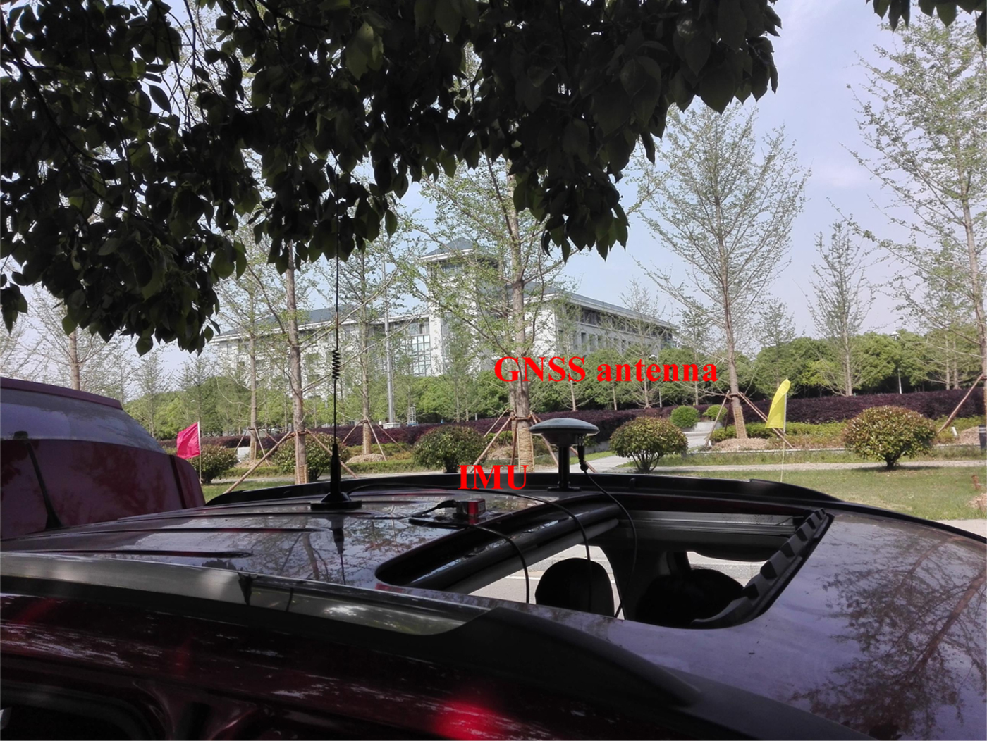
Figure 15. The experimental vehicle.

Figure 16. The trajectory of the experimental vehicle.
From 60 s to 80 s, a latitude error is introduced every 10 s; from 140 s to 160 s, a longitude error is introduced every 10 s. The performance of the two filtering methods is then compared. Figures 17, 18 and 19 show the position, velocity and attitude errors, respectively. From these figures, we found that after being processed by the adjusting method, the accuracy of the navigation results are enhanced by more than 20%.
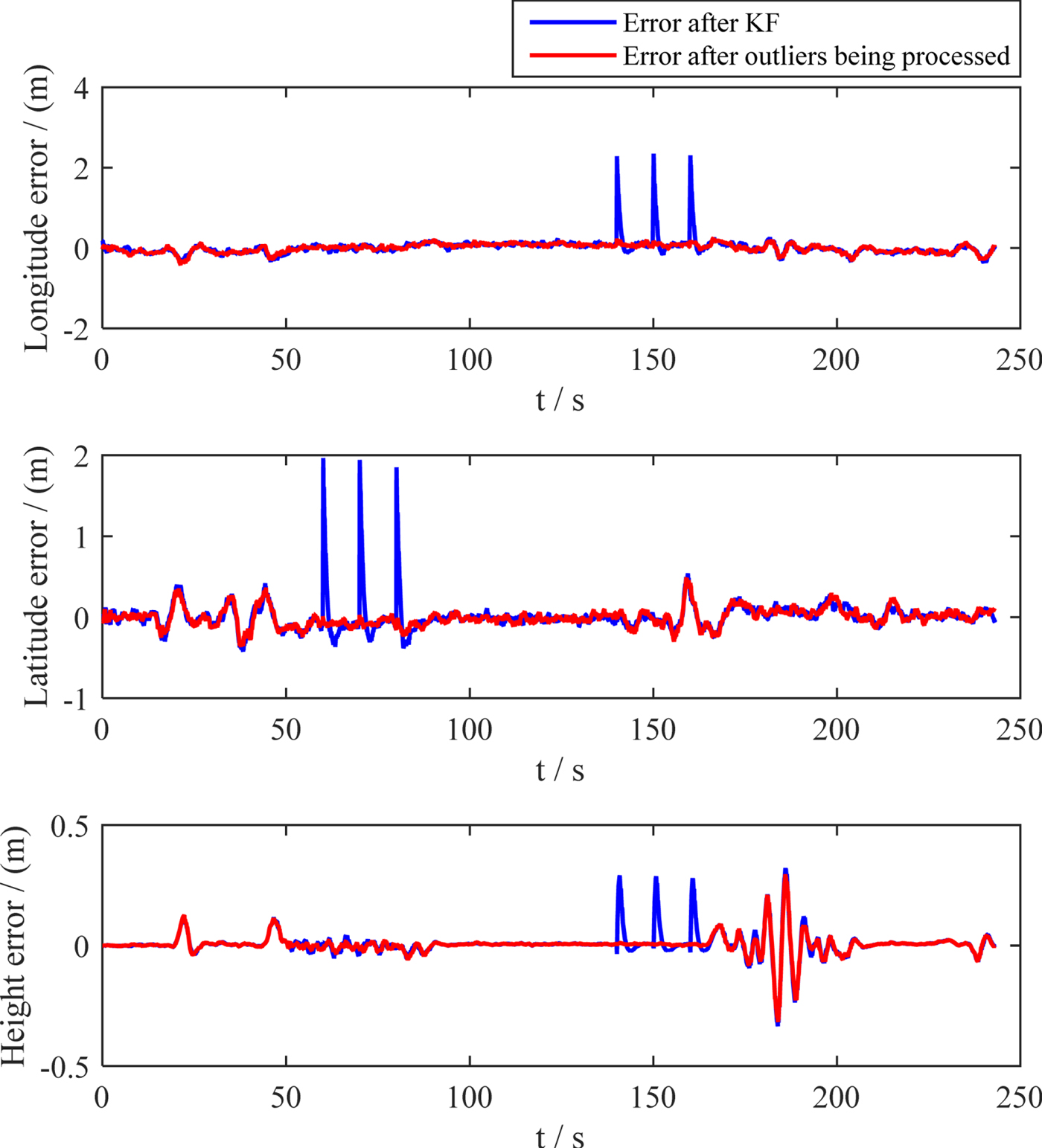
Figure 17. Position error contrast.
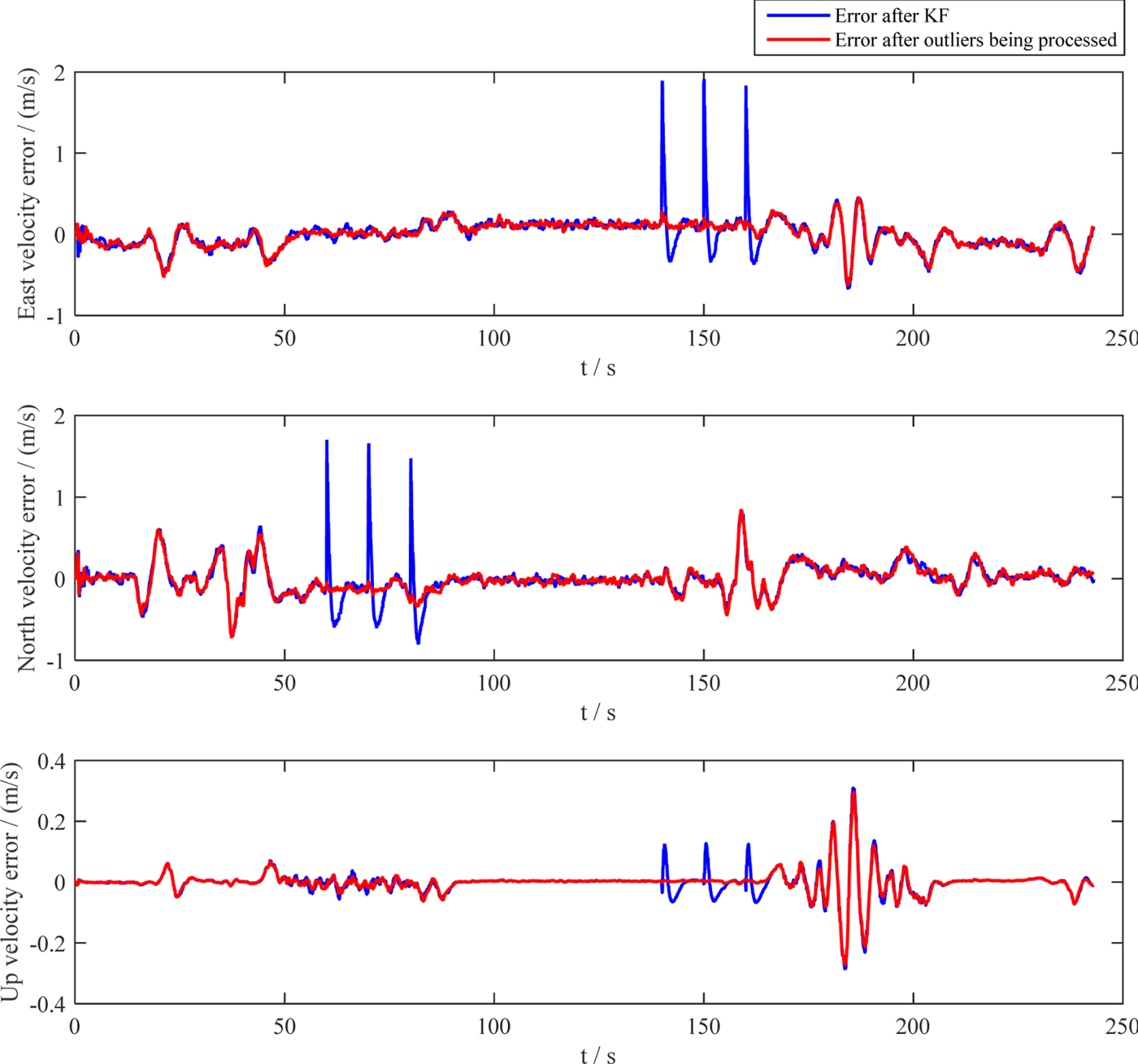
Figure 18. Velocity error contrast.

Figure 19. Attitude error contrast.
7. CONCLUSION
An INS and a GNSS receiver are combined by information filtering fusion in a GNSS/INS integrated navigation system. However, the GNSS is easily affected by observation outliers, and the conventional KF is of poor precision. A method based on the standard KF has been proposed to detect and suppress the influence of observation outliers. An innovation vector matrix, which obeys a χ2-distribution, is constructed using innovation vectors. Moreover, the χ2-test is carried out to detect the observation outliers. A scale factor is constructed using the parameters of the χ2-test and is used to reduce the corresponding filtering gain matrix. The simulation shows that there is no influence on the normal values and there is no fault or omission in detecting outliers. When there are big outliers, the performance of the system is enhanced by 90% for not only a single outlier but also for a set of consecutive outliers. Moreover, the time of the outlier's effect reduces by about a factor of five. When there are errors smaller than 25 m, the results will be optimised by 20% to 90% under different situations according to Table 1. For example, when 50 m continuous outliers are introduced every 10 s, the results of the position, velocity and attitude angle accuracies have increased by 93%. When the single outlier is 10 m, the resulting accuracy of position has increased by 21·8%. All the increments of accuracy after the dynamically adjusting filter gain method is applied are in the order of 20%~90%. Hence, the performance of the integrated navigation system is greatly improved, independently of the outlier's value.
ACKNOWLEDGEMENTS
The project is supported by the following funds: National Key Research and Development Program (2016YFD0702000), National Natural Science Foundation of China (61773113, 51477028).