1.0 INTRODUCTION
The high operating temperature characterizing the hypersonic flight regime is a long-term issue. Vehicles able to reach hypersonic speed are currently considered for both aeronautical (e.g. high-speed antipodal transportation systems) and space transportation purposes (e.g. reusable launcher stages and re-entry systems). In the past decades, several solutions have been investigated to protect vehicles from high heat fluxes penetrating the aeroshell as well as to withstand and control significant heat loads resulting from the exposure to a high-temperature environment for a relevant period of time. This generally led to the introduction of Thermal Protection Systems (TPS) and Thermal Control Systems (TCS) with peculiar features and functionalities depending on the specific applications.
In this context, the design and sizing of these on-board subsystems are very challenging activities for engineers, especially during the conceptual design phase. In particular, installation becomes an issue of primary importance when dealing with highly-integrated multifunctional subsystems. This is the case of the Thermal and Energy Management System (TEMS) to be integrated within the LAPCAT MR2 vehicle, a hypersonic cruiser project(Reference Steelant and Langener1).
In particular, this paper aims at providing a higher level of accuracy for turbopump physical modelling, i.e. for the geometrical characterization of turbomachinery for which detailed performance analyses have already been performed but for which geometrical characteristics still need to be defined. It has to be noted that performance and physical modelling techniques are quite different to each other mainly because of their different final aim. Performance analysis targets the identification of the performance behaviour in a quantitative way, while physical analysis is usually based on statistical approaches with a very different fidelity level. This discrepancy is a serious problem in the case of innovative and/or very complex products for which statistical analysis may not provide satisfactory results. This is the case for turbopumps and other components that the TEMS consists of that are characterised by a high power demand, and for which, the statistical approach demonstrated led to errors greater than 100%.
In order to overcome this problem, this paper works out a methodology for the development of semi-empirical models that allows for component sizing based on a set of operating conditions. The presented application to the TEMS relies on a subsystem architecture already presented in(Reference Steelant and Langener1) and for which advanced studies concerning both the vehicle and the on-board systems(Reference Steelant, Varvill, Defoort, Hannemann and Marini2) have already been published. Furthermore, this work provides a more complete understanding of the characteristics of TEMS and of its constituent components, paving the way for future studies of multifunctional systems for hypersonic vehicles.
After this short introduction, Section 2 briefly describes the existing estimation models that are available in literature, highlighting the reasons why they have been selected as reference documents but, at the same time, underlining the major issues to be overcome. Then, Section 3 describes the reference vehicle LAPCAT MR2 and provides some useful details on the envisaged point-to-point hypersonic mission and main operating points together with some highlights on the TEMS architecture and components. Section 4 represents the core of the article providing a description of the suggested methodology, and in parallel, Section 5 shows an example of the way in which this methodology can be applied to properly size turbopump assemblies. Results for the specific case of TEMS of the LAPCAT MR2 are presented in Section 6. Eventually, major conclusions and guidelines for future improvements are drawn.
2.0 EXISTING ESTIMATION MODELS
Different design and sizing models focusing on components usually exploited in a TEMS, or more generically in a TCS, are available in literature. In general, these sizing approaches are almost exclusively related to the definition of the components’ performance with only small contributions to the physical characterization of the components. This is a typical aspect of the conceptual design phase where active components (such as turbopumps, turbines and compressors) are mainly described by their operating parameters and conditions. Conversely, passive components are usually characterised on the basis of their physical features (e.g. weight and thickness for tanks(Reference Hart3) and pipes, etc.). This difference is mainly due to the fact that active components require a very detailed analysis of the design of the operational envelope and related aspects. For example, this is the case for turbomachinery for which it is usual to refer to the analysis of their working cycle, the effects on fluid characteristics and the induced pressure field, as well as to the general performance evaluation. During conceptual and preliminary design, easy and rapid mathematical formulations to characterize the components are required to perform high-level trade-off analyses upon the systems architecture. It is actually easier to associate numerical values to performance (often directly derived from high-level requirements and constraints) rather than defining quantitative estimations for physical parameters. For physical characterization, it is usual to adopt qualitative correlations, leading the designer to the definition of the components’ classes. For example, the diameter of turbomachinery is usually unknown during the conceptual design, but a rough idea of its sizing is given by the categorization of the component as axial, mixed or centrifugal flow.
It is also worth noticing that the performance characteristics differ mainly from physical ones as performance can be computed by means of exact and closed mathematical formulations, whilst physical aspects can only be hypothesized following best practices or general high-level requirements (usually depending on integration issues) acting as guidelines. Thus, it is quite common for active components to compute performance directly, whilst physical characteristics are derived through statistical approaches or legacy data coming from literature analysis and/or reports resulting from test campaigns. The so-called Weight Estimation Relationships (WERs) are in fact equations formulating mass derivation strategies based upon specific operational parameters of the components collected as a result of a generalised statistical analysis. This approach demonstrates some weaknesses, typically related to the quality of the component database upon which the statistical analysis is based. Even if it represents a good starting point to partially fill the gap between physical and performance derivation, it still remains far from an exact derivation (it is an approximated result).
Another critical problem of approximated models is the aging of the available data. Almost the whole set of studies on this topic refer to early reports coming from space agencies (e.g. NASA) that faced this problem early in 1960s. This may also affect the estimations, since coefficients and statistical drivers shall be subjected to actualization to provide correct results for modern components. This is one of the major showstoppers for highly innovative aerospace products that massively use breakthrough, advanced technologies. In these cases, the effect of aging is easier to tackle, introducing or updating proper coefficients and considering new production and manufacturing processes that may allow an increase in performance range. Moreover, regulation and certification policies are very useful guidelines for the definition of sizing algorithms.
In summary, considering this short digression over design approaches available in literature, it is possible to highlight the following:
– Performance and physical analyses are characterized by different levels of accuracy in the results, coming from exact / closed mathematical formulations and approximated estimations / qualitative hypotheses respectively.
– Physical estimations for active components available in literature are generally based upon statistical derivations, which are highly dependent on the technological characteristics of the historical period in which the data was gathered.
– Physical estimations for passive components are instead more reliable because they are referring to structural resistance and strength required to operate within the limits prescribed by the environmental conditions (and by regulations / standards)
It should be noted that many references propose semi-empirical formulations for the derivation of physical characteristics of the main components starting from assumptions and models related to their performance. However, performance and physical worlds remain quite separated in the references because the output from one analysis is seldom used for the other. Starting from these considerations, the approach here reported aims at overcoming the limits of the statistical derivation, suggesting the development of proper semi-empirical models to increase the accuracy of formulations leading to the estimations of the physical characteristics of mass, dimensions and volumes directly based upon operational parameters. The main difference with respect to the currently available methods is that, instead of using a database of components to build Estimation Relationships (ERs), physical data are derived directly from operating parameters (using those exact performance relationships in a convenient way) and then compared to available values for validation purposes only. The introduction of coefficients and corrective parameters is adopted only for those configuration and fabrication characteristics that cannot be included in other ways. The approach has demonstrated a general validity even if higher attention has been devoted to the definition of estimation models for active components.
Focusing in particular on turbopump characterization and design, a noticeable number of documents are available in literature. Apart from the pure theoretical derivation, available from different sources, attention has been focused on technical reports(4–6). These documents provide an overview of turbopump assemblies for liquid rocket engines together with an overview of the main parameters characterizing their performance. The turbopump databases included in the reports have been used as validation of the proposed model because the data presented in the documents are related to both performance and physical characteristics of real turbopumps. However, since the data was gathered in the 1970s, the database has been enriched with more recent machines generally exploited for rocket and space applications.
An interesting approach towards the identification of the physical characteristics of the machines is also provided in(Reference Epple, Durst and Delgado7), where a theoretical approach is suggested for the estimation of some dimensionless parameters of turbomachines based on the Cordier diagram. The main governing equations presented in(Reference Roncioni, Natale, Marini, Langener and Steelant11) the paper have been a starting point of the proposed work together with relationships relating the dimensionless parameters to each other. Semi-empirical methods for the estimation of the turbopump mass and volume(Reference Saunders8) have been selected as they provide a useful base for semi-empirical predictive models, besides considering some very specific operational ranges. In this paper, the authors propose the main equations for the determination of physical characteristics for a more general range of turbopumps by introducing some modifications to the original formulation presented in literature. Both relationships and their coefficients have been modified to be applicable to a wider spectrum of turbopumps, and the results have been compared to the original formulation for verification and validation purposes.
3.0 REFERENCE CASE STUDY: LAPCAT MR2 AND THE TEMS
3.1 LAPCAT MR2
Besides targeting the derivation of a methodology for a wider applicability, a real case study will also be addressed i.e. TEMS for the LAPCAT MR2 vehicle. The LAPCAT MR2 is a hypersonic cruiser concept resulting from multiple design optimizations performed within the European Projects LAPCAT I and LAPCAT II(Reference Steelant, Varvill, Defoort, Hannemann and Marini2). The vehicle is characterized by a waverider configuration, and it is equipped with six Air Turbo Rockets (ATRs)(Reference Fernández-Villacá, Paniaguá and Steelant9, Reference Meerts and Steelant10) and one Dual Mode Ramjet (DMR)(Reference Roncioni, Natale, Marini, Langener and Steelant11), which allows cruising at Mach 8 at an altitude above 33,000 m following the mission profile specified in Fig. 1. The engines use liquid hydrogen (LH2) as a fuel. A central intake that is equipped with several moveable ramps(Reference Meerts and Steelant10) allows the airflow to be driven either to the ATRs or to the DMR depending on the flight conditions.
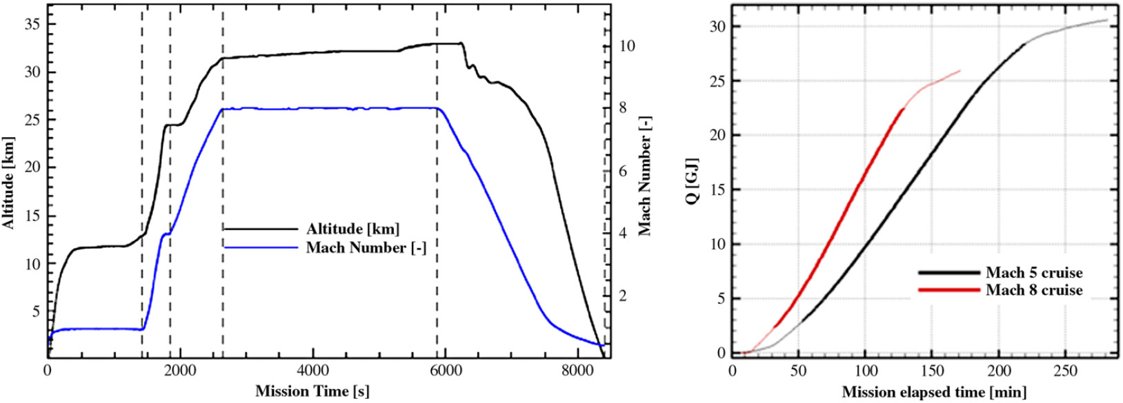
Figure 1. Reference mission for LAPCAT MR2, and integrated heat loads for different Mach(Reference Steelant and Langener1).
The vehicle is conceived to host 300 passengers providing a commercial anti-podal flight service across the globe, and it is characterized by a Maximum Take-Off Weight (MTOW) of about 400 tons.
3.2 Mission profile and operating conditions
Notably, the six ATRs operate up to Mach 4–4.5, whilst the DMR is used for hypersonic flight from Mach 4.5 up to Mach 8. The result is the mission profile reported in Fig. 1(Reference Langener, Erb and Steelant12), which is characterized by a first subsonic cruise, a supersonic ascent followed by the ATR switch-off as well as the ignition of the DMR and a subsequent hypersonic climb and cruise. The descent is then unpowered. The reference mission is Brussel–Sidney (direct route), characterized by a great circle distance of 16,700 km, and a flight time of about 2 hours and 45 minutes.
Notwithstanding the fact that the cruise altitude is almost three times the flight level selected by conventional aircraft, flying at this high speed produces high heat fluxes on the vehicle shell and, consequently, a high temperature on the skin layers. For the selected range of Mach numbers, the temperature of the pressure side of the aeroshell may reach 1,000–1,200 K in the worst condition. This leads to the adoption of proper materials for the TPS, belonging particularly to the ceramic family rather than the metallic one, especially for Mach higher than 4(Reference Fernandez Villace and Steelant13). This is more critical for sharp appendices (wing leading edges, canard, nacelles, etc.) and the lower part of the airframe (pressure side). However, flying at high speed may also be an advantage not only considering overall mission time, but also looking to the heat load accumulated by the vehicle indicated as the thermal paradox. It is in fact true that heat fluxes grow with increasing speed, but the heat has less time to penetrate the structure while the wall temperature does not increase proportionally with the total temperature. As an example, Fig. 1 shows the different heat load computations for a flight at Mach 5 and Mach 8, respectively(Reference Steelant and Langener1).
Apart from the external balance, other strategies shall be considered to control the amount of heat flowing through the shell to the internal compartment in order to guarantee proper survivability levels of both systems and payload. To face this problem, LAPCAT MR2 is also equipped with an innovative TEMS, which is designed to use the boil-off vapours coming from the evaporation of the LH2 within the tanks as the main cooling means for the cabin, the powerplant and the air-pack of the Environmental Control System (ECS). Moreover, the high-pressure liquid hydrogen is used to drive a dedicated turbine providing mechanical power to the devices of the TEMS itself, producing sufficient power margins for the other on-board subsystems.
3.3 Thermal and Energy Management Subsystem
The internal structure of the LAPCAT MR2 has been designed following a bubble-structure approach(Reference Steelant and van Duijn14), leading to a peculiar integration of passenger compartment, fuel tanks and propulsion subsystems in a non-conventional architecture. In particular, Fig. 2 clearly shows the very high level of integration of the different compartments, maximizing the exploitation of available room for subsystems integration, in a sort of modular approach(Reference Steelant and Langener1).
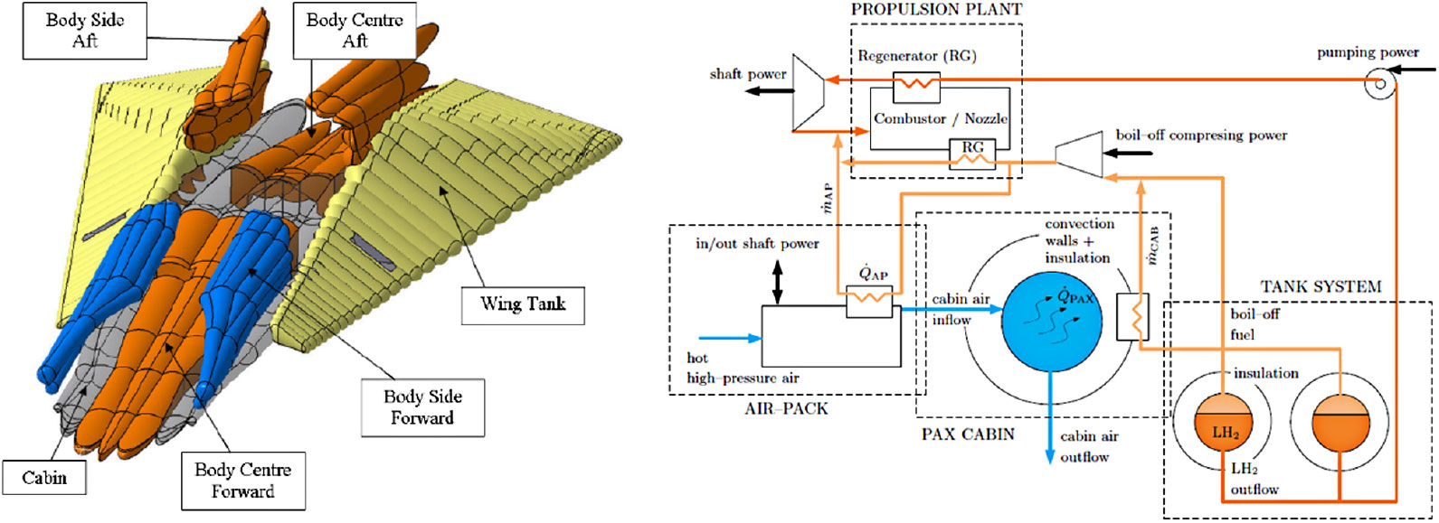
Figure 2. Tanks and cabin layout of LAPCAT MR2, and scheme of the TEMS of LAPCAT MR2(Reference Steelant and Langener1).
This assembly is characterized by large interface surfaces between the cabin itself and the tanks containing LH2 at a very low temperature (less than 20 K), leading to strategic advantages. Indeed, with this configuration, the heat coming from the aerodynamic heating is conducted across the aeroshell to the tanks producing a boil-off, which can be used within a dedicated thermodynamic cycle. The so-called TEMS, sketched in Fig. 2(Reference Steelant and Langener1), benefits from the boil-off produced in the LH2 tanks to directly cool down the passenger cabin. Moreover, the gaseous H2 is compressed and used as coolant within the air-pack of the ECS and the propulsion plant before the final injection within the combustion chamber.
The LH2 is pumped from the tanks to the engines, where it is used for cooling purposes and expanded within a dedicated turbine to produce mechanical power, before it is mixed with the boil-off and injected in the combustion chamber. The turbine provides mechanical power to the devices of the TEMS and offers the possibility of using the remaining power to satisfy the needs of other on-board systems.
The main active components of the TEMS (pump, turbine and compressor) have already been preliminary sized in specific working conditions (design point) as reported in(Reference Balland, Villace and Steelant15), providing the results shown in Table 1, which also reports the power budget.
Table 1 Design points of active components of the TEMS for LAPCAT MR2

4.0 METHODOLOGY
4.1 Methodology overview
As has been outlined in Section 2, performance and physical analyses differ from each other, mainly in terms of aims and fidelity levels, but for the conceptual design stage, it is very important to connect performances to physical characteristics of products. Of course, the derivation of correlations to estimate physical characteristics as a function of a set of operational parameters and performance is a very challenging and demanding task. Considering the complexity of this work and its multidisciplinary aspect, the exploitation of a systems engineering approach is proposed. This requires the focus moving progressively from the pure and limited technical engineering domain towards a multidisciplinary design. This is necessary to maximize the effectiveness of the entire vehicle rather than the efficiencies of each single component. In particular, the proposed approach aims at deriving a commonly integrated methodology that can be applied to a wide range of active and passive components to provide a reliable model for the prediction of their physical characteristics. Of course, each component should be analysed in detail, and proper sizing algorithms elicited, but the methodology presented here suggests a unique rationale of more general validity. Moreover, considering that these estimation relationships should be applicable from the conceptual and preliminary design phases, each mathematical model shall be conceived to be easily integrated within the overall design approach, exploiting e.g. the output of performance analysis as the main parameters for the mathematical formulations to predict mass, volume and dimensions of the devices. This will allow a standardization of the theoretical derivation approaches, the applicability to a wider range of components and a reduced impact on the workload. An overview of the overall derivation process is reported in Fig. 3.
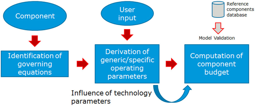
Figure 3. Proposed derivation process.
In particular, Fig. 3 reveals that the proposed methodology can be split into three different steps. The first one is related to the identification of the set of governing equations for the component under analysis. This can be done by referring to the applicable scientific literature describing the behaviour of specific devices by constituting relationships based upon the main operating parameters. These parameters are the core of the methodology allowing the computation of the power budget. A proper classification of these parameters is performed within the second phase of the method with the objective of analysing their impact on the governing equations. The identification of the relationships occurring among parameters and between variables and parameters allows expressing each variable (e.g. mass, diameter, etc.) as a function of this set of parameters. In the third phase, through the exploitation of results coming from empirical estimations, simulations or literature, it is possible to find out the proper mathematical formulations to represent those relationships occurring between each variable and its subset of parameters.
Before entering into the detail of the methodology, the following subsection aims at suggesting classification criteria for drivers.
4.2 Preliminary drivers’ classification
In this context, different kinds of parameters, or ‘drivers’, can be identified depending on the variables they represent and on the physical phenomenon under evaluation. In particular, for the purposes of this study, four different categories have been identified:
Generic Operating Parameters (GOP); they represent the main performance of a component (e.g. rotating speed of the machine, mass flow, pressure rise, efficiency, etc.). They are referred to as ‘generic’ because different kinds of components can be described by use of them, as they describe the basic physical occurring phenomena.
Specific Operating Parameters (SOP); different from GOP, they are particular to a specific kind of machine (or at least of a family of machines). They can often be expressed in a non-dimensional way to allow comparisons between similar components. They may also assume the aspect of simple coefficients conceived to represent the main characteristic of a machine with a single value or through a couple of variables (e.g. specific speed and specific diameter).
Secondary Parameters (SP); they are usually a function of SOP, and they can be related to the characteristics of the subparts of the components (e.g. the inducer of a pump, the blade of a turbine, etc.)
Technology Parameters (TP); they are able to reflect the technology maturation level of a component. They may be expressed through coefficients and corrective factors, allowing a higher flexibility of the model (since they may be adopted to enlarge the limits of the correlations) even if causing a sort of discontinuity with the aim of the ‘exact formulation’ of the estimations.
Eventually, when dealing with the development of these estimation models, the limited availability of data should be taken into account, as it may impose a pruning of the parameters to be used in conceptual design phases. In fact, since the model is conceived to host a specific set of variables in its equations, it is important for the user to have access to this kind of information or to proper suggestions or formulations to estimate the missing data (e.g. it could be difficult to ask the user for a specific value of the tangential speed of the flow over an impeller blade, being easier to ask for general performance like the mass flow and then implementing a proper equation to derive it where it is necessary in the model). Thus, it is very important to define which subset of drivers among the GOP, the SOP and the SP shall be used to make the model applicable at the proper design level.
Then, the identified parameters are used in building up proper equations allowing the computation of the so-called system mass and volume budgets. Actually, power budgets may be computed as well, since, in general, for active components, the expression of power produced and consumed is directly related to their GOP. Moreover, the third phase is also the right place to perform the validation of the model, benefitting from the data available in literature concerning the physical characteristics of the components and comparing the results with the data coming from the real world. This can also lead to the modification of the correlations in case proper corrective trends are identified within the data.
Looking at the formal representation of the equations, it is possible to say that, since the governing equations G can be usually represented as in Equation (1)
 \begin{equation}
G=g\left(GOP,SOP\right)
\label{eqn1}
\end{equation}
\begin{equation}
G=g\left(GOP,SOP\right)
\label{eqn1}
\end{equation}
the final estimation relationship F will be assembled in Equation (2) as a function of the aforementioned drivers
 \begin{equation}
F=f\left(G,\ SP,\ TP\right)
\label{eqn2}
\end{equation}
\begin{equation}
F=f\left(G,\ SP,\ TP\right)
\label{eqn2}
\end{equation}
where
 \begin{equation}
SP=h\left(SOP\right)
\label{eqn3}
\end{equation}
\begin{equation}
SP=h\left(SOP\right)
\label{eqn3}
\end{equation}
This brings us to the formalization of the estimation relationship
 ${\mathcal F}$
in the generic form:
${\mathcal F}$
in the generic form:
 \begin{equation}
{\mathcal F}=f[ g(GOP,SOP),h(SOP),\ TP]
\label{eqn4}
\end{equation}
\begin{equation}
{\mathcal F}=f[ g(GOP,SOP),h(SOP),\ TP]
\label{eqn4}
\end{equation}
5.0 TURBOPUMPS
This section aims at describing the step-by-step application of the generic methodology presented in Section 4 to the specific case of turbopump assemblies.
5.1 Identification of governing equations (Step 1)
Turbopumps are widely used devices for different aerospace applications, from engine feed (typically for rockets) to thermodynamic cycles that require moderate to high power. Different models for performance estimations are present in literature, starting from theoretical derivation of the operational parameters(4, 16). Moreover, some legacy data, referring to some specific design points, are available and can be used to statistically derive mass and sizing models(5, 8). But unfortunately, as has already been highlighted Section 2, pure statistical models are not applicable for the purposes of this paper as they do not establish any relationships between physical characteristics and operating parameters.
An in-depth analysis of the existing literature is essential to have a clear view of the wide spectrum of turbopump architectures that can be envisaged. A typical and useful characterization of these machines can be performed through the computation of two main parameters, the specific speed
 $N_s$
and the specific diameter
$N_s$
and the specific diameter
 $D_s$
defined respectively as in Equations (5) and (6)(Reference Sobin4).
$D_s$
defined respectively as in Equations (5) and (6)(Reference Sobin4).
 \begin{gather}
N_s=\frac{NQ^{\frac{1}{2}}}{H^{\frac{3}{4}}}\label{eqn5}\end{gather}
\begin{gather}
N_s=\frac{NQ^{\frac{1}{2}}}{H^{\frac{3}{4}}}\label{eqn5}\end{gather}
 \begin{gather}
D_s=\frac{DH^{{1/4}}}{Q^{{1/2}}}
\label{eqn6}\end{gather}
\begin{gather}
D_s=\frac{DH^{{1/4}}}{Q^{{1/2}}}
\label{eqn6}\end{gather}
where
N is the rotating speed (rpm).
Q is the volumetric flow rate (usually expressed in imperial units as (gpm)).
H is the head rise (ft) (as far as imperial units are concerned).
D is the diameter of the machine (ft) (as far as imperial units are concerned).
Through these numbers, different machines can be compared directly on a single diagram, known as the Balje diagram, that represents a sort of map upon which many other coefficients can be plotted (as a function of these two main parameters). The different types of turbopump architectures can be identified on the diagram depending on the ranges of
 $N_s$
and
$N_s$
and
 $D_s$
(Fig. 4).
$D_s$
(Fig. 4).

Figure 4. Balje and Cordier diagrams for turbopumps.
As an example, the head and flow coefficients
 $\psi $
, Equation (7), and
$\psi $
, Equation (7), and
 $\varphi $
, Equation (8), can be derived from the aforementioned numbers since
$\varphi $
, Equation (8), can be derived from the aforementioned numbers since
 \begin{gather}
\psi =\frac{gH}{u^{2}}\propto \frac{H}{N^{2}D^{2}}\label{eqn7}\end{gather}
\begin{gather}
\psi =\frac{gH}{u^{2}}\propto \frac{H}{N^{2}D^{2}}\label{eqn7}\end{gather}
 \begin{gather}
\varphi =\frac{v}{u}\propto \frac{Q}{ND^{3}}
\label{eqn8}\end{gather}
\begin{gather}
\varphi =\frac{v}{u}\propto \frac{Q}{ND^{3}}
\label{eqn8}\end{gather}
where
g is the gravity constant (9.81 (m/
 ${{\rm s}}^{2}$
))
${{\rm s}}^{2}$
))u is the peripheral velocity (m/s))
v is the absolute velocity (m/s)

Note that once the head rises, the volumetric flow rate, the rotational speed of the machine and the characteristic velocities of the flow have been computed, the main data for machine characterization are already available from the operational standpoint.
Considering that these values are strictly related to the operating conditions of the machine, a simplification of the design problem has been achieved(Reference Epple, Durst and Delgado7) by looking at the definition of the optimum operating condition of a turbomachinery working at
 $Q_{opt}$
,
$Q_{opt}$
,
 $\triangle p_{opt}$
,
$\triangle p_{opt}$
,
 $N_{opt}$
and optimum efficiency. In analogy with the definition of
$N_{opt}$
and optimum efficiency. In analogy with the definition of
 $N_s$
and
$N_s$
and
 $D_s$
, similar constituting parameters, namely the speed
$D_s$
, similar constituting parameters, namely the speed
 $\sigma $
and diameter
$\sigma $
and diameter
 $\delta $
numbers (Equations (9) and (10)), refer to a simpler diagram known as the Cordier diagram (Fig. 4).
$\delta $
numbers (Equations (9) and (10)), refer to a simpler diagram known as the Cordier diagram (Fig. 4).
 \begin{gather}
\sigma =0,355{\Omega }_s\label{eqn9}\end{gather}
\begin{gather}
\sigma =0,355{\Omega }_s\label{eqn9}\end{gather}
 \begin{gather}
\delta =\frac{\sqrt{\pi }}{{2}^{{3}/{4}}}D_s
\label{eqn10}\end{gather}
\begin{gather}
\delta =\frac{\sqrt{\pi }}{{2}^{{3}/{4}}}D_s
\label{eqn10}\end{gather}
with
 \begin{equation}
{\Omega }_s=\frac{\Omega Q^{{1/2}}}{Y^{{3/4}}}
\label{eqn11}
\end{equation}
\begin{equation}
{\Omega }_s=\frac{\Omega Q^{{1/2}}}{Y^{{3/4}}}
\label{eqn11}
\end{equation}
where
-
${\Omega }_s$
is the specific speed with reference to
$\Omega $
-
$\Omega $
is the rotating speed (rad/s)
Q is the volumetric flow rate
$({{\rm m}}^{3}$
/s)-
$Y=gH$
is the specific head (J/kg)


Consequently, the expression of head and flow coefficients can be re-arranged as in Equations (12) and (13).
 \begin{gather}
\psi =\frac{1}{2{\sigma }^{2}{\delta }^{2}}\label{eqn12}\end{gather}
\begin{gather}
\psi =\frac{1}{2{\sigma }^{2}{\delta }^{2}}\label{eqn12}\end{gather}
 \begin{gather}
\varphi =\frac{1}{\sigma {\delta }^{3}}
\label{eqn13}\end{gather}
\begin{gather}
\varphi =\frac{1}{\sigma {\delta }^{3}}
\label{eqn13}\end{gather}
Equations (5) and (6) can be then identified as the main governing laws for turbopumps and have the formal representation of
 \begin{equation}
{\mathcal G}=g(GOP)=g\left(\sigma,\delta \right)=g\left(N,Q,H,D\right)
\label{eqn14}
\end{equation}
\begin{equation}
{\mathcal G}=g(GOP)=g\left(\sigma,\delta \right)=g\left(N,Q,H,D\right)
\label{eqn14}
\end{equation}
5.2 Derivation of operating parameters (Step 2)
In this section, the approach followed to derive the mathematical formulation of operating parameters characterizing turbopumps from governing equations is described. For the purposes of this work, the second group of governing equations, Equations (9) and (10), is selected and re-arranged in order to be compatible with the hypotheses here described. The model described in(Reference Epple, Durst and Delgado7) is taken as reference.
The volumetric flowrate Q, rotational speed
 $\Omega$
and head rise H (or pressure rise
$\Omega$
and head rise H (or pressure rise
 $\triangle p$
/ specific head Y) is supposed to be known by the user, since a first evaluation of the performance should be available. In this way, the computation of specific speed
$\triangle p$
/ specific head Y) is supposed to be known by the user, since a first evaluation of the performance should be available. In this way, the computation of specific speed
 ${\Omega }_s$
and speed number
${\Omega }_s$
and speed number
 $\sigma $
is straightforward as indicated in Equations (9) and (11). Equation (10) can be used to derive the reference diameter as the function of
$\sigma $
is straightforward as indicated in Equations (9) and (11). Equation (10) can be used to derive the reference diameter as the function of
 $\delta $
through the afore mentioned parameters (Fig. 5).
$\delta $
through the afore mentioned parameters (Fig. 5).
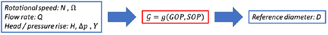
Figure 5. Variables flowchart for input / output of governing equation of turbopumps.
The diameter number
 $\delta $
is unknown at this stage. In order to overcome this problem, it is possible to benefit from the equation that relates
$\delta $
is unknown at this stage. In order to overcome this problem, it is possible to benefit from the equation that relates
 $\sigma $
and
$\sigma $
and
 $\delta $
through the maximum efficiency of the machine
$\delta $
through the maximum efficiency of the machine
 ${\eta }_{opt}$
, Equation (15), which shall be hypothesized by the user. In fact, depending on the required efficiency, it is possible to derive the characteristic dimensions of the machine working within the previously specified operating conditions.
${\eta }_{opt}$
, Equation (15), which shall be hypothesized by the user. In fact, depending on the required efficiency, it is possible to derive the characteristic dimensions of the machine working within the previously specified operating conditions.
 \begin{equation}
{\eta }_{opt}=1-\frac{1}{{4}{\delta }^{2}}\left(\frac{{4}}{{\delta }^{2}}+\frac{1}{{\sigma }^{2}}\right)
\label{eqn15}
\end{equation}
\begin{equation}
{\eta }_{opt}=1-\frac{1}{{4}{\delta }^{2}}\left(\frac{{4}}{{\delta }^{2}}+\frac{1}{{\sigma }^{2}}\right)
\label{eqn15}
\end{equation}
Imposing
 $\triangle ={\delta }^2$
, Equation (16) can be obtained:
$\triangle ={\delta }^2$
, Equation (16) can be obtained:
 \begin{equation}
{4}{\sigma }^{2}+\triangle +4{\sigma }^{2}\left({\eta }_{opt}-1\right){\triangle }^{2}=0
\label{eqn16}
\end{equation}
\begin{equation}
{4}{\sigma }^{2}+\triangle +4{\sigma }^{2}\left({\eta }_{opt}-1\right){\triangle }^{2}=0
\label{eqn16}
\end{equation}
This is a second order algebraic equation, which provides two families of results, as seen in Equations (17) and (18):
 \begin{gather}
{{\triangle }_{1}{\mathbf \ =}\delta }_{1,2} =\pm \sqrt{\frac{-1-\sqrt{{1-64}{\sigma }^{{4}}\left({\eta }_{opt}{-1}\right)}}{{8}{\sigma }^{2}\left({\eta }_{opt}{-1}\right)}}\label{eqn17}\end{gather}
\begin{gather}
{{\triangle }_{1}{\mathbf \ =}\delta }_{1,2} =\pm \sqrt{\frac{-1-\sqrt{{1-64}{\sigma }^{{4}}\left({\eta }_{opt}{-1}\right)}}{{8}{\sigma }^{2}\left({\eta }_{opt}{-1}\right)}}\label{eqn17}\end{gather}
 \begin{gather}
{{\triangle }_{2}=\delta }_{{3,4}}=\pm \sqrt{\frac{{-1+}\sqrt{{1-64}{\sigma }^{{4}}({\eta }_{opt}{-1)}}}{{ 8}{\sigma }^{2}({\eta }_{opt}{-1)}}}
\label{eqn18}\end{gather}
\begin{gather}
{{\triangle }_{2}=\delta }_{{3,4}}=\pm \sqrt{\frac{{-1+}\sqrt{{1-64}{\sigma }^{{4}}({\eta }_{opt}{-1)}}}{{ 8}{\sigma }^{2}({\eta }_{opt}{-1)}}}
\label{eqn18}\end{gather}
Only positive values have physical relevance. Moreover, looking at the conditions of existence, it is possible to notice that the only possible solution is
 ${\delta }_1$
, as in Equation (19),
${\delta }_1$
, as in Equation (19),
 $\forall \sigma \ne 0$
.
$\forall \sigma \ne 0$
.
 \begin{equation}
{\delta }_{1}=\sqrt{\frac{{-1-}\sqrt{{1-64}{\sigma }^{{4}}({\eta }_{opt}{-1)}}}{{8}{\sigma }^{2}({\eta }_{opt}{-1)}}}
\label{eqn19}
\end{equation}
\begin{equation}
{\delta }_{1}=\sqrt{\frac{{-1-}\sqrt{{1-64}{\sigma }^{{4}}({\eta }_{opt}{-1)}}}{{8}{\sigma }^{2}({\eta }_{opt}{-1)}}}
\label{eqn19}
\end{equation}
In this way, it is possible to obtain the formulation for the diameter, applying equations (10) and (6) in series. Moreover, with the derivation of
 $\delta $
, it is also possible to compute head and flow coefficients
$\delta $
, it is also possible to compute head and flow coefficients
 $\psi $
,
$\psi $
,
 $\varphi $
(Equations (7) and (8)) and the subsequent flow velocities (Equation (7)). Upon conclusion of this step, the governing equations for turbopumps can be obtained as in Equation (20).
$\varphi $
(Equations (7) and (8)) and the subsequent flow velocities (Equation (7)). Upon conclusion of this step, the governing equations for turbopumps can be obtained as in Equation (20).
 \begin{equation}
\left\{ \begin{array}{c}
\sigma =\frac{1}{\sqrt{\pi }}\frac{\Omega Q^{{1/2}}}{({2Y)}^{{\rm 3/4}}} \\
{\eta }_{opt}=1-\frac{1}{{4}{\delta }^{2}}\left(\frac{{4}}{{\delta }^{2}}+\frac{1}{{\sigma }^{2}}\right) \end{array}
\right.
\label{eqn20}
\end{equation}
\begin{equation}
\left\{ \begin{array}{c}
\sigma =\frac{1}{\sqrt{\pi }}\frac{\Omega Q^{{1/2}}}{({2Y)}^{{\rm 3/4}}} \\
{\eta }_{opt}=1-\frac{1}{{4}{\delta }^{2}}\left(\frac{{4}}{{\delta }^{2}}+\frac{1}{{\sigma }^{2}}\right) \end{array}
\right.
\label{eqn20}
\end{equation}
Once the machine is fully characterized, it is possible to move to the physical characterization of the turbopump assembly and related components following the model proposed in(Reference Saunders8). Table 2 summarizes the main results of this methodology step. The different estimation relationships to derive turbopump dimensions and mass can be computed starting from this group of parameters.
Table 2 List of operating parameters for turbopump governing equations

5.3 Turbopump assembly arrangements
This section aims at performing a review of the existing turbopump architectures with the final goal of underlining in which way the different locations of the components affect the sizing equations. Depending on the specific type of coupling between turbine and pumps, three different turbopump assemblies can be distinguished: direct driven, geared or dual-shaft turbopumps.
As summarized in Table 3, when a single turbine directly drives both propellant pumps by means of a common shaft, two different configurations are possible. Indeed, the turbine can be located at the shaft end, in a back-to-back configuration, or it can be simply placed between pumps. The first configuration is the most interesting for the applications dealt with in this paper. An example of this type of configuration is represented by the turbopump of the Rocketdyne F-1 rocket, which was used on the first stage of Saturn V. For both the configurations, the turbopump diameter will be driven by the larger diameter among the oxidizer pump, the fuel pump and the turbine. Considering the serial alignment of all the elements, the axial dimension of the overall assembly can be identified putting together their single length and adding a term to take into account extra length due to element connections.
Table 3 High-level estimations strategies for the derivation of dimensions of different turbopump assemblies

Considering geared turbopump arrangements, three different configurations can be envisaged, depending on the type of geared connections. The pancake type is applied in case of speed differentials between pumps and turbines and requires the exploitation of different reduction gears. An example of a pancake configuration is the YLR87 –AJ-7 turbopump that was used on the Titan launch vehicle. In case the two propellant pumps are rotating at the same speed but differently with respect to the turbine, the gears should be used to connect the pumps shaft to the turbine shaft; this configuration is usually referred to as off-set turbine. An example of the off-set turbine configuration is the turbopump assembly of the MA-5 booster stage. The last type of geared turbopump is the single-geared. The single-geared turbopump is used when the turbine can directly lead the fuel pump, but gears are required to be placed in between the two pumps due to different rotating speeds. This configuration is present in the RL10A-3-3 turbopump. As summarised in Table 3, both the diameter and the length of the assemblies are strongly affected by the arrangement. In particular, the off-set turbine configuration may be the most compact in terms of diameter.
Dual-shaft configurations are widely used in aerospace, especially in rocket propulsion systems. For example, they have been used for the Space Shuttle Main Engine (SSME) High Pressure Oxygen Turbopumps (HPOTOP) and SSME High Pressure Fuel Turbopumps (HPFTP), the Saturn V second stage J-2 turbopumps and the more recent Vulcain, Vulcain II and Vinci Turbopumps, which are to be used on board Ariane 5 and Ariane 6. In this case, two different arrangements can be envisaged depending on the way in which hot gases are fed into the turbine: series or parallel dual shafts. In this case, as summarised in Table 4, the diameter and length estimation should be performed separately for the two propellant turbopumps.
Table 4 High-level estimation strategies for the derivation of dimensions of dual-shaft turbopumps

As example, in order to characterize the turbopumps within the database, Table 8 shows some existing turbopump architecture with reference to the assemblies’ schematic reported in Table 4.
Table 5 Examples of existing turbopumps with reference to the assemblies’ schematic

5.4 Turbopump components sizing and budgets (Step 3)
5.4.1 Diameter estimation (Model 1)
The reference diameter is one of the most important physical parameters of the turbopumps when trying to characterize its volume and mass. This is due to the fact that, in general, the diameter of the machine can be related to the other physical features by means of semi-empirical models. This section addresses useful semi-empirical formulations for the estimation of the diameter of the different components of a turbopump. Considering the equations referred to in the previous section, it is crystal clear that the components with a higher impact on the definition of the overall turbopump diameter are the pumps and turbines. However, in order to obtain more accurate results, especially in terms of mass budget, equations for the estimation of the other components are suggested too.
The diameter of the pump component can be estimated considering the maximum between the impeller diameter and the inducer. However, in all the analysed cases, the impeller contribution is always higher than the inducer one, when this last component is present.
The impeller diameter is directly related to the specific diameter reported in Equation (6). But from the analysis of the various type of existing pumps, the inverse formulation (reported in Equation (21)) derived from Equation (6) is only able to differentiate between machines with different operating fluids and cannot differentiate between information related to the impact of number of stages of the impeller or of the impeller constructional type.
 \begin{equation}
D_{P_{imp}}'=\frac{D_sQ^{\frac{1}{2}}_m}{Y^{\frac{1}{{4}}}_m}
\label{eqn21}
\end{equation}
\begin{equation}
D_{P_{imp}}'=\frac{D_sQ^{\frac{1}{2}}_m}{Y^{\frac{1}{{4}}}_m}
\label{eqn21}
\end{equation}
Indeed, in the case of multistage impellers, it shall be considered that they are mounted on the same shaft and, thus, they run at the same rotational speed. Moreover, since they are acting in series, they are supposed to handle the same fluid flow as an ideal single-stage, with the same total developed head. As a consequence, the impeller diameter of a multistage configuration should be smaller. Thus, the previous equation can be corrected by reference to the affinity laws stating that:
The pump volume flow rate varies directly with the rotational speed
The pump-developed head varies directly as the square of speed
and assuming that the developed head developed by each stage of the impeller is equal to the head developed by the ideal single-stage machine divided for the number of stages, the following Equation (22) is suggested.
 \begin{equation}
D_{P_{imp}}=\frac{D_sQ^{\frac{1}{2}}_m}{Y^{\frac{1}{{4}}}_m}\sqrt{\frac{1}{{{(n}_{stage})}_{imp}}}
\label{eqn22}
\end{equation}
\begin{equation}
D_{P_{imp}}=\frac{D_sQ^{\frac{1}{2}}_m}{Y^{\frac{1}{{4}}}_m}\sqrt{\frac{1}{{{(n}_{stage})}_{imp}}}
\label{eqn22}
\end{equation}
Considering possible different configurations for each of these elements, the authors suggest that it would be preferable to express all the missing contributions as proper percentages with respect to the impeller diameter, giving suggestions on how to tune these percentages depending on the characteristics of the element that is considered. It is worth noting that the identification of proper factors representing the impact of the different components on the pump diameter has been based on an in-depth investigation of several components. Thus, the pump diameter can be estimated as in Equations (23) and (24):
 \begin{gather}
D_P=D_{P_{imp}}\left(1+k_{P_{D/other}}\right)\label{eqn23}\end{gather}
\begin{gather}
D_P=D_{P_{imp}}\left(1+k_{P_{D/other}}\right)\label{eqn23}\end{gather}
 \begin{gather}
k_{P_{D/other}}=k_{D/diff}+k_{D/inlet}+k_{D/outlet}+k_{D/misc}+k_{D/integration}
\label{eqn24}\end{gather}
\begin{gather}
k_{P_{D/other}}=k_{D/diff}+k_{D/inlet}+k_{D/outlet}+k_{D/misc}+k_{D/integration}
\label{eqn24}\end{gather}
where
 $k_{D/diff}$
is the contribution of the diffuser to the diameter estimation (see Table 8);
$k_{D/diff}$
is the contribution of the diffuser to the diameter estimation (see Table 8);
 $k_{D/inlet}$
is the contribution of the inlet to the diameter estimation;
$k_{D/inlet}$
is the contribution of the inlet to the diameter estimation;
 $k_{D/outlet}$
is the contribution of the inlet to the diameter estimation;
$k_{D/outlet}$
is the contribution of the inlet to the diameter estimation;
 $k_{D/misc}$
is the contribution of other elements (connectors, etc.) to the diameter estimation (this value is strictly related to the under-design turbopump);
$k_{D/misc}$
is the contribution of other elements (connectors, etc.) to the diameter estimation (this value is strictly related to the under-design turbopump);
 $k_{D/integration}$
is the contribution of components integration (e.g. casing, insulation, etc.) to the estimation (a value of 0.3 is suggested).
$k_{D/integration}$
is the contribution of components integration (e.g. casing, insulation, etc.) to the estimation (a value of 0.3 is suggested).
The impact of the diffuser onto the diameter estimation can vary 0.1–1.2, and it depends on the type of geometry adopted to build the diffuser vane. Indeed, the diffuser’s aim is to convert the velocity head in the pressure head with as little turbulence as possible. This is done in one or more passages surrounding the impeller. Three major types of impeller might be identified:
annular diffuser (
$k_{D/diff}$
lower that 0.5)volute diffuser (
$k_{D/diff}$
lower than 0.8)diffusing vane (
$k_{D/diff}$
higher than 0.8)


The impact of inlet and outlet vanes, as well as of the other secondary elements, is strictly related to the geometry of the turbopump assembly. However, typical numbers, for different configurations, are reported in Table 6.
Table 6 Coefficient used for turbopump diameter estimation and results obtained using the different models

Whilst the constructional architecture of the impeller does not affect the diameter, it is considered in the next section because it significantly affects the length of the pump.
5.4.2 Diameter estimation (Model 2)
In literature, other interesting models have already been presented. In particular, the model presented by the Royal Air Force(Reference Saunders8) has been considered interesting and a good additional reference model to compare the proposed results and validate it.
Following the suggestions reported in the RAF model, the diameter of the pump can be evaluated starting from the consideration that the delivery pressure of the pump can be estimated as the sum of two different contributions: the dynamic and the static pressure.
 \begin{equation}
p=\frac{1}{2g}\rho \left(U^{2}-u^{2}\right)+\frac{\psi \rho U^{2}}{2g}
\label{eqn25}
\end{equation}
\begin{equation}
p=\frac{1}{2g}\rho \left(U^{2}-u^{2}\right)+\frac{\psi \rho U^{2}}{2g}
\label{eqn25}
\end{equation}
where
U is the speed at the tip of the pump impeller;
u is the speed at the impeller hub;
-
$\psi $
pressure recovery factor (0.2 suggested value(Reference Saunders8));
U is the peripheral velocity at the outer radius of the impeller (ft/s);
u is the peripheral velocity at the hub of the impeller (ft/s);
g is the gravity constant (32.18 (ft/
${{\rm s}}^{2}$
)).


Considering that the two speeds can be easily put in relationship with the radius at the hub or tip section of the impeller blade (see Equations 26 and 27) and remembering that the radius can be expressed by Equation (28),
 \begin{gather}
u=2\pi r_{impeller}n\label{eqn26}\end{gather}
\begin{gather}
u=2\pi r_{impeller}n\label{eqn26}\end{gather}
 \begin{gather}
U=2\pi R_{impeller}n
\label{eqn27}\end{gather}
\begin{gather}
U=2\pi R_{impeller}n
\label{eqn27}\end{gather}
the radius at the hub can be expressed as:
 \begin{equation}
r_{impeller}=\sqrt{\frac{\dot{m}}{\rho \pi u}}
\label{eqn28}
\end{equation}
\begin{equation}
r_{impeller}=\sqrt{\frac{\dot{m}}{\rho \pi u}}
\label{eqn28}
\end{equation}
Equation (29) expresses the external radius estimation equation:
 \begin{equation}
R_{impeller}=\sqrt{{C_i}_{1}\frac{p}{n^{2}\rho }+{C_i}_{2}\frac{\dot{m}}{\rho u}}
\label{eqn29}
\end{equation}
\begin{equation}
R_{impeller}=\sqrt{{C_i}_{1}\frac{p}{n^{2}\rho }+{C_i}_{2}\frac{\dot{m}}{\rho u}}
\label{eqn29}
\end{equation}
Thus, comparing Equation (22) to Equation (29), it is possible to understand the meaning of the
 $C_{i1}$
and
$C_{i1}$
and
 $C_{i2}$
coefficients in the original formulation.
$C_{i2}$
coefficients in the original formulation.
 \begin{gather}
C_{i1}=\frac{g}{2{\pi }^{2}\left(1+\psi \right)}\left[\frac{ft}{s^{2}}\right]\label{eqn30}\end{gather}
\begin{gather}
C_{i1}=\frac{g}{2{\pi }^{2}\left(1+\psi \right)}\left[\frac{ft}{s^{2}}\right]\label{eqn30}\end{gather}
 \begin{gather}
C_{i2}=\frac{1}{\pi \left(1+\psi \right)}\quad[-]
\label{eqn31}\end{gather}
\begin{gather}
C_{i2}=\frac{1}{\pi \left(1+\psi \right)}\quad[-]
\label{eqn31}\end{gather}
However, this formulation, as per the one suggested in(Reference Saunders8), does not allow one to take into account the effect of the number of stages of the impeller. Thus, the overall pump formulation will also include the correction due to the number of stages. The additional contributions, mainly due to the presence and impact of the other components are evaluated following the same suggestions implemented in Equation 32.
 \begin{equation}
D_P= 2R_{impeller}\left(1+k_{P_{D/other}}\right)
\label{eqn32}
\end{equation}
\begin{equation}
D_P= 2R_{impeller}\left(1+k_{P_{D/other}}\right)
\label{eqn32}
\end{equation}
The following table reports the major results related to the application of both models for the estimation of the diameter of some existing turbopumps developed for aerospace propulsion systems. As can be noted, even if these two models start with different hypotheses, they are both able to estimate diameter values that correspond very closely to the real data available from literature.
In addition, the diameter of the different subparts can be evaluated as follows (Equations (33–36)).
 \begin{gather}
D_T=\frac{k_{2}}{n}\label{eqn33}\end{gather}
\begin{gather}
D_T=\frac{k_{2}}{n}\label{eqn33}\end{gather}
 \begin{gather}
D_B=2D_{Shaft}\label{eqn34}\end{gather}
\begin{gather}
D_B=2D_{Shaft}\label{eqn34}\end{gather}
 \begin{gather}
D_P={2k}_{3}R_{impeller}\label{eqn35}\end{gather}
\begin{gather}
D_P={2k}_{3}R_{impeller}\label{eqn35}\end{gather}
 \begin{gather}
D_s=2D_{Shaft}
\label{eqn36}\end{gather}
\begin{gather}
D_s=2D_{Shaft}
\label{eqn36}\end{gather}
where
 $k_2$
and
$k_2$
and
 $k_3$
are constants.
$k_3$
are constants.
5.4.3 Length estimation
A similar approach is suggested here to evaluate the overall length of the turbopump on the basis of its constituent components. In particular, considering the different possible assembly configurations, overall turbopump length can be estimated considering the formulations reported in Table 7. This section aims to assess how entering in the details of the different elements contributes to the overall turbopump weight.
Table 7 Coefficients used for turbopump length computation and related results

In the most generic case, where all the components are present, the turbopump length (Equation (37)) can be evaluated as the sum of several elements:
 \begin{equation}
l_{TP}=l_{imp}+l_{pb}+l_{ind}+l_b+l_t+l_{out}+l_{other}
\label{eqn37}
\end{equation}
\begin{equation}
l_{TP}=l_{imp}+l_{pb}+l_{ind}+l_b+l_t+l_{out}+l_{other}
\label{eqn37}
\end{equation}
where
-
$l_{imp}$
is the impeller length at the hub;
-
$l_{pb}$
is the length of the pre-burner that might be present (usually expressed as a percentage with respect to
$l_{imp}$
);
-
$l_{ind}$
is the length of the inducer;
-
$l_b$
is the length of the bearings;
-
$l_t$
is the length of the turbine;
-
$l_{out}$
is the length of the outlet section of the turbine.


The length of the impeller can usually be estimated on the basis of the mass flow that the pump should handle, whilst remembering that the length of the impeller is proportional to the inlet pump diameter (Equation (38)):
 \begin{equation}
l_{imp}=\frac{r_{in}}{2}
\label{eqn38}
\end{equation}
\begin{equation}
l_{imp}=\frac{r_{in}}{2}
\label{eqn38}
\end{equation}
where the inlet radius (
 $r_{in}$
) can be estimated as it follows in Equation (39)
$r_{in}$
) can be estimated as it follows in Equation (39)
 \begin{equation}
r_{in}=\sqrt{\frac{\dot{m}}{\rho u\pi }}
\label{eqn39}
\end{equation}
\begin{equation}
r_{in}=\sqrt{\frac{\dot{m}}{\rho u\pi }}
\label{eqn39}
\end{equation}
Again, this formulation does not allow the consideration of multistage impellers and does not reflect the type of impeller blade. Thus, the authors suggest the evaluation of
 $l_{imp}$
through Equation (40).
$l_{imp}$
through Equation (40).
 \begin{equation}
l_{imp}=k_{imp}n_{stages}\sqrt{\frac{\dot{m}}{\rho u\pi }}
\label{eqn40}
\end{equation}
\begin{equation}
l_{imp}=k_{imp}n_{stages}\sqrt{\frac{\dot{m}}{\rho u\pi }}
\label{eqn40}
\end{equation}
where
 $k_{imp}$
is a coefficient that takes into account the blade shape. In the case of a pure radial impeller,
$k_{imp}$
is a coefficient that takes into account the blade shape. In the case of a pure radial impeller,
 $k_{imp}=0.7$
is suggested while moving to mixed-flow types towards Francis construction, and higher values should be adopted (1.2 mixed-flow and 2 for Francis type).
$k_{imp}=0.7$
is suggested while moving to mixed-flow types towards Francis construction, and higher values should be adopted (1.2 mixed-flow and 2 for Francis type).
The contributions of other elements are usually estimated as a percentage with respect to the impeller length, apart from bearings and turbines, for which equations based upon best design practices (from textbooks and experience) may be used (see Equation (41))
 \begin{gather}
l_b=2D_{shaft}=2\frac{u_{shaft}}{({\pi n}_T)}=2\frac{0.1\ u_T}{({\pi n}_T)}\label{eqn41}\end{gather}
\begin{gather}
l_b=2D_{shaft}=2\frac{u_{shaft}}{({\pi n}_T)}=2\frac{0.1\ u_T}{({\pi n}_T)}\label{eqn41}\end{gather}
 \begin{gather}
l_t=0.083\ n_{stages}[ ft]
\label{eqn42}\end{gather}
\begin{gather}
l_t=0.083\ n_{stages}[ ft]
\label{eqn42}\end{gather}
where
-
$D_{shaft}$
is the diameter of the rotating shaft (ft);
-
$u_T$
tubine speed at the blade tip (m/s);
-
$n_T$
is the rotating speed of the turbine (rpm).
Eventually, the turbopump length (37) can be expressed as follows:


 \begin{equation}
l_{TP}=l_{imp}(1+k_{L/ind}+k_{L/pb}+k_{L/out}+k_{L/other})+{l_b+l}_t
\label{eqn43}
\end{equation}
\begin{equation}
l_{TP}=l_{imp}(1+k_{L/ind}+k_{L/pb}+k_{L/out}+k_{L/other})+{l_b+l}_t
\label{eqn43}
\end{equation}
This model has been applied to the same set of turbopump assemblies, and the input and results are collected in Table 7.
5.4.4 Mass, volume and power budgets estimation
Then, a high-level estimation of the volume can be executed by simply multiplying the diameter of the machine and its length (45).
 \begin{gather}
V_p=\frac{l_P\pi D^{2}}{4}\label{eqn44}\end{gather}
\begin{gather}
V_p=\frac{l_P\pi D^{2}}{4}\label{eqn44}\end{gather}
 \begin{gather}
M_{TP}={I{(M}_P}_{casing}+{M_P}_{impeller}+{M_T}_{rotor}+{M_T}_{shaft}+M_B)
\label{eqn45}\end{gather}
\begin{gather}
M_{TP}={I{(M}_P}_{casing}+{M_P}_{impeller}+{M_T}_{rotor}+{M_T}_{shaft}+M_B)
\label{eqn45}\end{gather}
The masses of pump casing, Equation (46), and impeller, Equation (47), as well as the turbine mass can be derived from similar considerations.
 \begin{gather}
M_{P_{casing}}={\rho }_{cP}\left(\pi R^{2}_{impeller}\right)l_P\label{eqn46}\end{gather}
\begin{gather}
M_{P_{casing}}={\rho }_{cP}\left(\pi R^{2}_{impeller}\right)l_P\label{eqn46}\end{gather}
 \begin{gather}
M_{P_{impeller}}={\rho }_PR^{2}_{impeller}b_{impeller}\label{eqn47}\end{gather}
\begin{gather}
M_{P_{impeller}}={\rho }_PR^{2}_{impeller}b_{impeller}\label{eqn47}\end{gather}
 \begin{gather}
{M_T}_{rotor}=l_TR^{2}_T{\rho }_r
\label{eqn48}\end{gather}
\begin{gather}
{M_T}_{rotor}=l_TR^{2}_T{\rho }_r
\label{eqn48}\end{gather}
In particular, considering the results of the validation process and a subsequent sensitivity analysis, the coefficient has been expressed as
 \begin{equation}
I=I_N\cdot I_{\dot{m}}
\label{eqn49}
\end{equation}
\begin{equation}
I=I_N\cdot I_{\dot{m}}
\label{eqn49}
\end{equation}
Suggested values for these coefficients are reported in Tables 8 and 9.
I and
 ${k'}_1$
can be grouped as those technology parameters (TP) that can be identified for the different families of turbopump.
${k'}_1$
can be grouped as those technology parameters (TP) that can be identified for the different families of turbopump.
Eventually, the power budget for the overall turbopump can be evaluated with the simple Equation (50), where the power required is the product of volumetric flow rate and delivery pressure with an additional efficiency.
Table 8 Values of
 ${{\boldsymbol{I}}}_{\mathbf N}$
coefficient
${{\boldsymbol{I}}}_{\mathbf N}$
coefficient

Table 9 Values of
 ${{\boldsymbol{I}}}_{\dot{{{\boldsymbol{m}}}}}$
coefficient
${{\boldsymbol{I}}}_{\dot{{{\boldsymbol{m}}}}}$
coefficient

a This range of values is due to the impact of pressure rise. Lower
 $I_{\dot{m}}$
values are suggested for low values of
$I_{\dot{m}}$
values are suggested for low values of
 $\Delta p$
.
$\Delta p$
.
 \begin{equation}
P_{TP}=\frac{pQ}{{\eta }_P}
\label{eqn50}
\end{equation}
\begin{equation}
P_{TP}=\frac{pQ}{{\eta }_P}
\label{eqn50}
\end{equation}
5.5 Validation of the model
Tables 10 and 11 contain the database of the turbopumps used for the validation of the models presented in Section 5.4. Unfortunately, only a subset of these turbopumps has been used for the validation of the sizing models due to the lack of constructional details. However, the application to this set of turbomachinery reports error margins of the Politecnico di Torino (POLITO) model lower than 30% but, in many cases, under 10%. The difference in the accuracy of the results may depend on the skill of the user to set those parameters related to the machines configuration properly. Of course, this demonstrates that the unavailability of detailed constructional drawings is a hampering factor for this approach.
Table 10 Turbopump database

a These turbopumps have not been considered for the final mass estimations because constructional drawings are not available.
Table 11 Turbopump analysis results comparison

Results obtained through the application of the presented model have been compared with those coming from a statistical model presented in literature(Reference Sobin4) and with available real data. Figure 7 and Tables 10 and 11 report the results of the validation process. As it is possible to notice from Fig. 7, the statistical approach seems not to be applicable for high power turbopumps. This confirms that new algorithms (like the one proposed in this paper) are necessary when dealing with breakthrough innovations and out-of-boundary performance. However, the mass estimation of YLR87-A1-7 presents similar results with both POLITO and statistical estimations. This is mainly because of the fact that due to the very complex assembly, this turbopump has a power density (kg/kW) with respect to pumps with similar power demand (Vulcain 1 - Ox), and for this reason, the statistical analysis significantly overestimates the Vulcain 1 - Ox while it catches the YLR87-A1-7.
The results prove the flexibility of the approach, even if some differences between the computed and the real values still remain. The different results are in line with the statistical model(Reference Sobin4), and in the majority of the cases, they show better correlation. It is also interesting to see how the estimations seem to be more accurate than the statistical formulation.
It is worth noting that whilst the differences in mass estimation with respect to real data are relevant, the model presented in this paper gives better results in the majority of the cases if compared to the other considered statistical approaches. Of course, it is clear that the next steps in terms of research activities to be performed is the identification of suitable corrective factors properly fitted to take into account the differences in the architectures of the components.
5.6 Sensitivity analysis
A sensitivity analysis is set out here to support the validation of the methodology as well as to guide the users throughout the setting of parameters of the model suggested in this paper. In order to achieve this goal, the results of a sensitivity analysis performed for the Space Shuttle Main Engine Turbo Pumps (SSME-TP) are reported (Tab 11 and Tab 12).
Table 12 Sensitivity analysis results – Impact of parameters on TP diameter estimation

As can be noted, in many cases, the local optimum value for a single parameter is not selected i.e. there is a certain difference between the predicted diameter or mass (dots) with respect to the real data (dashed lines). This is due to the fact that the main purpose of the model is to achieve a proper TP assembly mass estimation; thus, the method is not aiming at the optimisation of the single parameters or elements of the TP. However, this sensitivity analysis is extremely useful to understand the impact of each parameter on the final budget, but it is important to note that the value selection for each parameter shall be carried out looking at the combined effect of all the parameters on the final objective function that, in this case, is the mass of the overall TP assembly.
6.0 LAPCAT TURBOPUMP SIZING
The semi-empirical model presented in the previous sections has been applied to the size of the turbopump of the LAPCAT MR2. Reference (Reference Balland, Villace and Steelant15) has been a valuable source of inputs for this case study. However, the operational ranges are not the only values required. Indeed, as already reported and discussed in Fig. 6, it is also necessary to make reasonable design assumptions, mainly related to the constructional characteristics of the overall assembly.
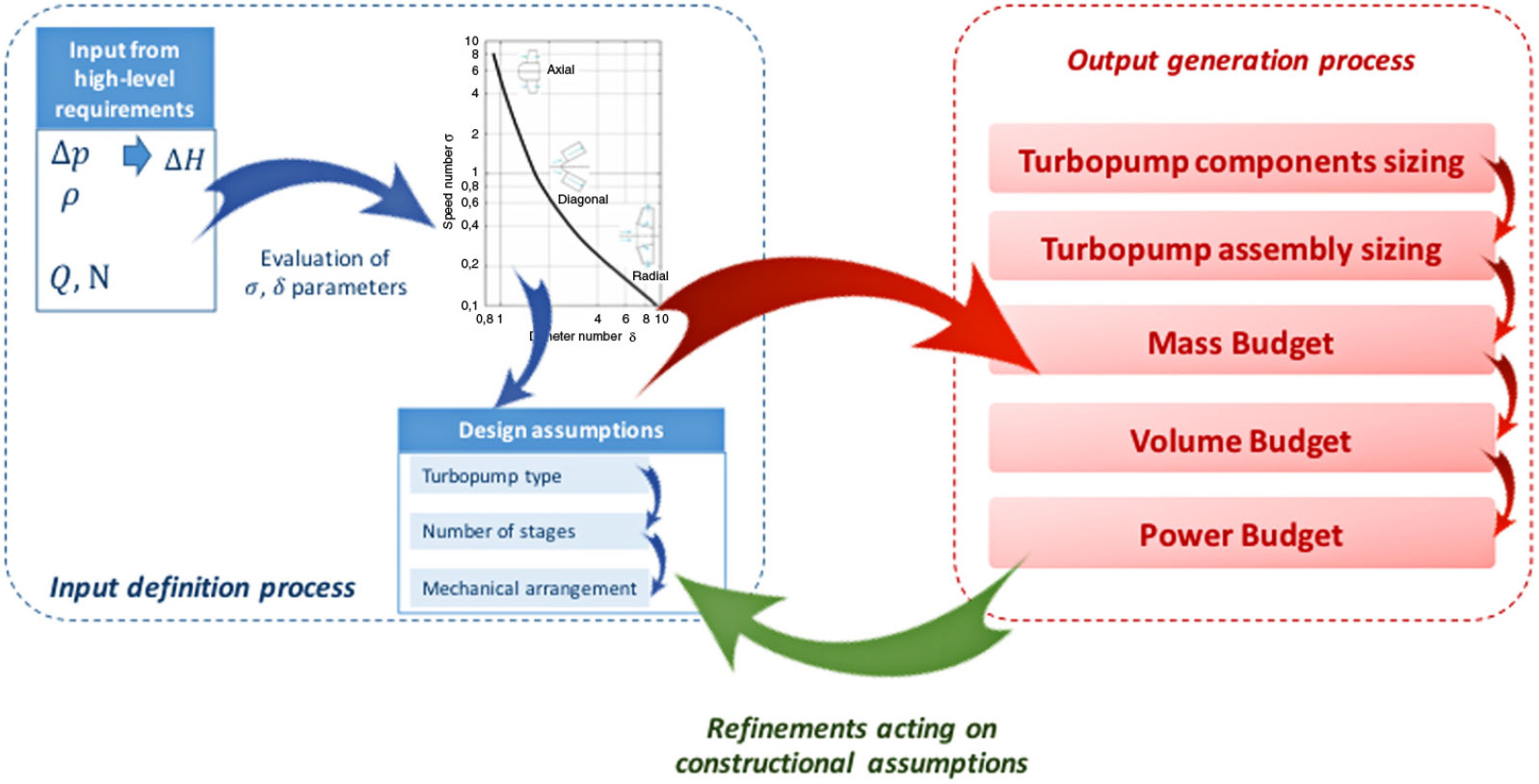
Figure 6. Activity flow-chart to summarise the input-output definition processes.
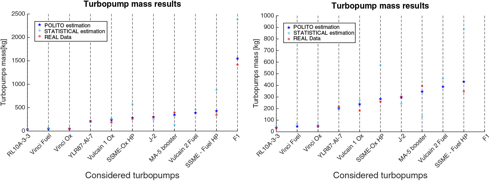
Figure 7. Summary of turbopumps mass computation and comparison with statistical approach.
Table 14 summarizes both inputs and design assumptions for the LAPCAT MR2. Starting from these operating ranges and assuming an efficiency value of 0.7, in line with the turbopumps of the database considered, the Cordier diagram has been plotted for different N values within the hypothesized range. As previously highlighted, higher N values move the turbopump towards a higher speed number
 $\sigma $
and lower diameter number
$\sigma $
and lower diameter number
 $\delta $
(Fig. 8). Considering the ranges of
$\delta $
(Fig. 8). Considering the ranges of
 $\sigma $
and
$\sigma $
and
 $\delta $
, it is possible to note that the points are in the class of radial flow. Thus, a radial configuration is suggested here. Then, different architectures are considered for what concerns the number of stages of the pump. Ultimately, a direct driven turbopump type has been hypothesized. This assumption might be reviewed in future works, where the integration issues of the overall subsystem will be analysed in-depth.
$\delta $
, it is possible to note that the points are in the class of radial flow. Thus, a radial configuration is suggested here. Then, different architectures are considered for what concerns the number of stages of the pump. Ultimately, a direct driven turbopump type has been hypothesized. This assumption might be reviewed in future works, where the integration issues of the overall subsystem will be analysed in-depth.
Table 13 Sensitivity analysis results – Impact of parameters on TP length estimation

Table 14 LAPCAT MR2 – Input and assumptions for turbopump sizing

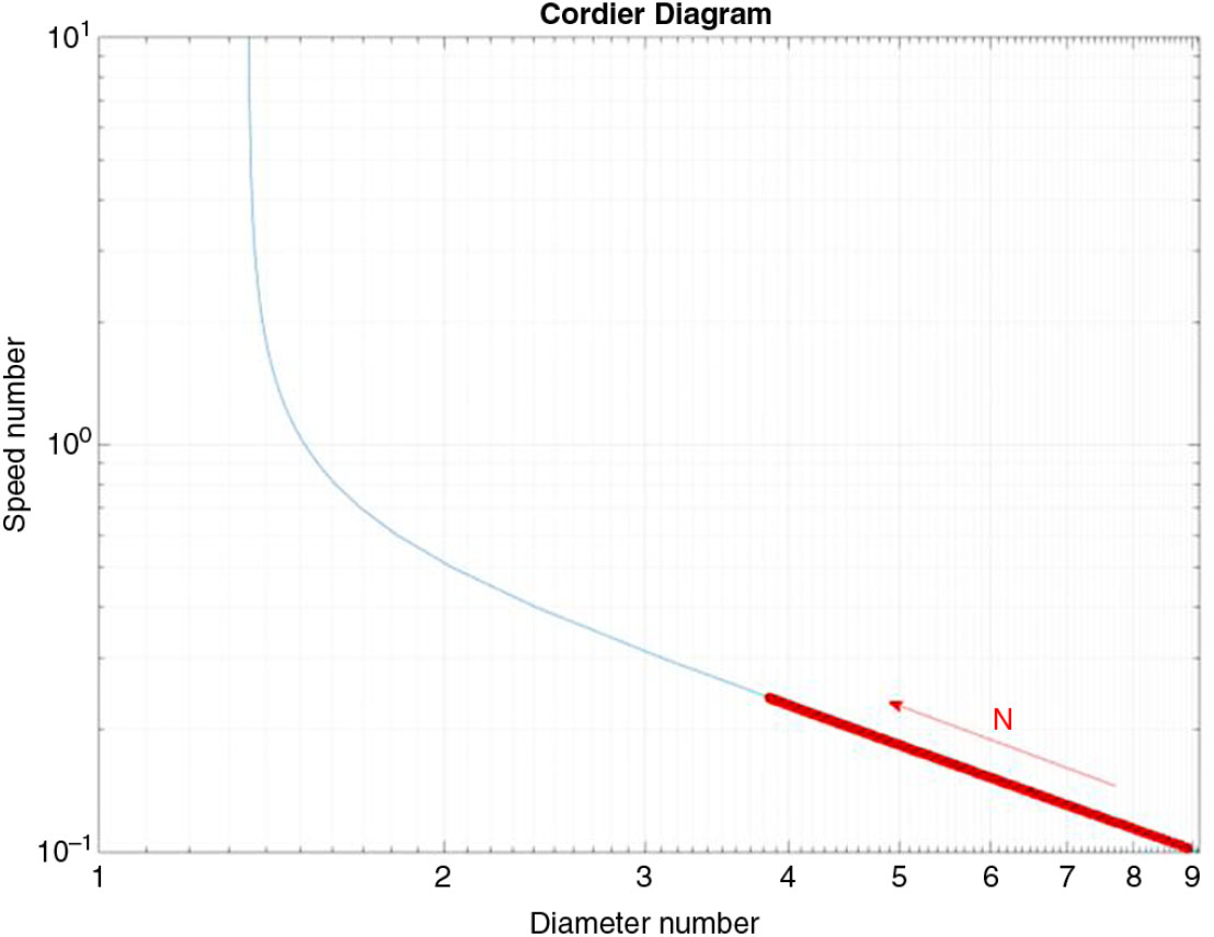
Figure 8. Cordier Diagram for LAPCAT MR2 turbopump.
In Section 6.1, the major results for the LAPCAT MR2 vehicle are reported and commented upon.
Table 15 LAPCAT MR2 – outputs of turbopump sizing

Physical characteristics are not subject to changes during operation, as occurs in relation to performance factors, which are dependent on the specific working conditions (e.g. flow rate, pressure drop, power consumption, velocities of the flow, etc.). However, the characterization of the machine depends on the selected design point, which will affect the final arrangement of the component in terms of mass and other physical characteristics. For this reason, it is crucial to properly select the design point of the considered device not only looking at the performance range, but also referring to its final mechanical configuration (e.g. a certain component may be enabling from the performance point of view but leading to an unfeasible solution because of excessive weight or volume). In Section 6.1, the main results of the sensitivity analysis are discussed, with a special focus on the identification of possible trends of physical characteristics with design conditions. Apart from the capability of theoretically predicting the final arrangement of the machine, the analysis of the effects of the design operating point is one of the crucial advantages of the proposed approach and represents a remarkable benefit of this research activity.
6.1 Sizing example
Considering the trends reported in the previous subsections, an example of sizing for the turbopump of LAPCAT MR2 has been carried out hypothesizing a high rotational speed (
 $N=35,000\ rpm$
), the highest mass flow (
$N=35,000\ rpm$
), the highest mass flow (
 $\dot{m}=100\frac{kg}{s}$
) rate and head rise (
$\dot{m}=100\frac{kg}{s}$
) rate and head rise (
 $\Delta P=80\ bar$
) and a single-stage impeller and a two-stage turbine in a direct driven configuration. Moreover, additional assumptions related to more constructional details should be done in order to properly estimate diameter, length and, eventually, mass budget.
$\Delta P=80\ bar$
) and a single-stage impeller and a two-stage turbine in a direct driven configuration. Moreover, additional assumptions related to more constructional details should be done in order to properly estimate diameter, length and, eventually, mass budget.
As far as the fuel pump is concerned, the hypothesized LAPCAT MR2 turbopump baseline configuration is characterized by a single-stage pump with frontal inlet and an inducer. Moreover, in order to maximize the developed pressure head (in line with Vulcain TP), a volute diffuser has been selected.
Table 16 LAPCAT MR2 – sensitivity analysis on turbopump sizing

These assumptions are collected in Table 15 together with the results.
It is worth noticing that 100 kg/s is the maximum flow rate that LAPCAT MR2 will need during a typical mission. However, this happens in very specific conditions such as during cruise when the required mass flow rate of liquid hydrogen is about 20 kg/s. Thus, one would not opt for one single pump for different reasons. Redundancy is a key driver to splitting the pump unit into different smaller ones. These can be placed optimally at the lowest points of the various tanks on-board while also being interconnected. The pump size is usually determined following consideration of the need for redundancy and avoidance of single-point failure. This is an element that still needs to be worked out in the future to ensure a workable and safe operational solution. Table 16 reveals that, hypothesizing a constant eta coefficient (
 $\eta =0.7$
), the exploitation of a higher number of turbopumps to provide the requested mass flow is not convenient in terms of mass increase. However, the exploitation of two turbopumps, instead of a single one, may bring noticeable benefits from the safety standpoint, although producing a non-negligible mass increase. The assumption of a constant efficiency coefficient will be relaxed in the future when optimization cycles will be performed in order to re-evaluate the ideal eta coefficient of the different turbomachinery in the various mission phases.
$\eta =0.7$
), the exploitation of a higher number of turbopumps to provide the requested mass flow is not convenient in terms of mass increase. However, the exploitation of two turbopumps, instead of a single one, may bring noticeable benefits from the safety standpoint, although producing a non-negligible mass increase. The assumption of a constant efficiency coefficient will be relaxed in the future when optimization cycles will be performed in order to re-evaluate the ideal eta coefficient of the different turbomachinery in the various mission phases.
7.0 CONCLUSIONS
A major goal of this paper was the development of a general methodology to support the sizing of innovative TCS for high-speed transportation systems. This methodology should be sufficiently general to be exploited for the derivation of ERs of sizing characteristics as well as mass, volume and power budgets for both active and passive components(Reference Ferretto, Vercella, Fusaro, Viola, Fernandez Villace and Steelant17). Following the suggested approach, ad-hoc semi-empirical models, relating to the geometrical size, mass, volume and power features of each component to operating conditions, have been derived by starting with an in-depth literature review. At the beginning of this paper, a general methodology to tackle the highlighted problems has been proposed and then it has been applied to the derivation of a semi-empirical parametric model for turbopump sizing.
For the sake of clarity, a real test case has been considered. The overall turbopump sizing algorithms have been applied to the TEMS for the LAPCAT MR2 vehicle as an example of a highly integrated multifunctional subsystem. The estimations led to a turbopump of noticeable dimensions still considering some conservative assumptions. Indeed, in the future, a review of the presented algorithms, both in their formulation and in the suggested values for the parametric coefficients, will be performed. This activity will allow us to consider future productive scenarios where new available materials or technologies could be introduced into existing designs.