1. Introduction
Recent decades have been accompanied with a rapid increase in natural catastrophic events, for instance, tsunamis, earthquakes, and forest fires. Consequently, the number of claims from catastrophic insurance has quite often become massive and sometimes outweighed the capacity of the insurance firm. This increase in insurance losses has forced insurance firms to rely more on financial derivatives to hedge their exposure against the catastrophic risk. One of the most popular derivatives is the catastrophe equity put option, which is analogous to a vanilla put option, with an additional feature that the option holder can only exercise his right if the total catastrophic losses exceed a certain level. As a result, pricing a catastrophe option is more involved in comparison pricing a vanilla put option.
The breakthrough article by Cox published in 2004 [Reference Cox, Fairchild and Pedersen4] serves as a cornerstone in the pricing of catastrophe options. The paper developed a pricing model assuming that the underlying process is governed by geometric Brownian motion augmented with an additional negative jump in case of a catastrophe event. In contrast with Cox et al. [Reference Cox, Fairchild and Pedersen4] where only the number of catastrophe events played a role in pricing but not the size of the losses, Jaimungal and Wang [Reference Jaimungal and Wang9] extended their framework by including stochastic interest rates and modeling the losses by a compound Poisson process. This implies that the size of the loss due to a catastrophic event also affects the share price. Chang and Hung [Reference Chang and Hung2] derived an analytic pricing formula assuming the dynamics of the underlying to be governed by a Lévy process with finite activity. Later on, various modifications have been put forward by several authors. Lin and Wang [Reference Lin and Wang11] utilized a penalty function approach to investigate perpetual American catastrophe put options. Chang et al. [Reference Chang, Lin and Yu3] studied the pricing of catastrophe options assuming a Markov-modulated Poisson process governing the catastrophic events, whereas Kim et al. [Reference Kim, Kim and Kim10] assumed that catastrophe losses are correlated to the underlying stock price. Yu [Reference Yu15] modeled the underlying asset by an exponential jump process with two compound Poisson processes. Wang [Reference Wang14] studied catastrophe options by taking into consideration the expectations of the insurance firm regarding the future realized variance.
Although the aforementioned articles provide analytical formulae for the pricing of catastrophe equity put options, their valuation methodology involves evaluating several layers of infinite sums and  $n$-fold convolutions of the distribution functions. For instance, the pricing formula of Chang and Hung [Reference Chang and Hung2] involves evaluating the infinite sum of expressions that include integral of
  $Hh$ functions and confluent hyper-geometric function. Although these articles derived a closed-form pricing formula, their final expression for the price is an infinite sum which is nothing but expectation over the loss process. In other words, despite being in a closed-form, their pricing formulas are equivalent to Monte-Carlo simulation over paths of the loss process. Furthermore, these pricing formulae depend on a particular choice of the model for the underlying asset and catastrophe loss. These observations motivate the need for an approach that is more simplified and if possible independent of the underlying modeling framework. Fortunately, we come out with a way to overcome the difficulties mentioned above using a characteristic function approach.
In this article, we derive a general pricing formula for catastrophe put options in terms of the joint characteristic function of the underlying asset and catastrophe losses under any modeling framework as long as the joint characteristic function can be derived analytically. The use of characteristic function in option pricing dates back to Carr and Madan [Reference Carr and Madan1]. A similar approach in the multivariate case has been applied in Griebsch and Wystup [Reference Griebsch and Wystup5] but in a different context. They considered pricing of exotic options with payoffs depending on finitely many spot values such as fader options and discretely monitored barrier options. We follow a similar approach in the pricing of catastrophe options. The main contribution of this article is Theorem 2.1 which provides a closed-form exact formula that utilizes a significantly simplified approach of characteristic function and hence circumvent the evaluation of infinite sums of  $n$-fold convolutions of probability density functions reported in the literature. Moreover, the final form of the obtained pricing formula was versatile in dealing with the specific model for the underlying process, and hence can be conveniently used by market practitioners. To demonstrate the application of the pricing formula, we consider a jump-diffusion model with negative exponential jumps and stochastic jump intensity, and analytically obtain the target characteristic function. Since the maturity of a catastrophe option can be more than a year, we consider a stochastic interest rate environment. Finally, the accuracy of the newly derived formula is demonstrated by comparing the option prices calculated with our formula to those obtained from Monte-Carlo simulation.
The rest of the paper is organized as follows. Section 2 derives a general closed-form expression for the price of catastrophe put option in terms of the joint characteristic function of the underlying asset and catastrophe losses. To present an application of the proposed approach, Section 3 discusses two different modeling frameworks where we introduce the dynamics of the underlying stock, the catastrophe losses, and the interest rate. Then, we derive an analytical formula for the joint characteristic function of the underlying price and catastrophe losses. Section 4 validates the proposed closed-form pricing formula through the numerical experiments by comparing the option prices obtained using the proposed formula to those obtained using Monte-Carlo simulations. Section 5 concludes the article.
2. Pricing catastrophe put option with a stochastic interest rate
In this section, we derive a general closed-form expression for the price of European catastrophe put option in terms of the joint characteristic function of the underlying asset and the loss process.
2.1. General pricing formula
We begin with a finite time horizon  $T > 0$. Assume that the filtered probability space
  $(\Omega ,\mathcal {F},Q,\mathcal {F}_{t\in [0,T]})$ models the uncertainty in the economy and
  $Q$ is the risk neutral probability measure. Let
  $\{S_t,\ t\geq 0\}$ denote the share value process and
  $L_t=-\sum _{i=1}^{N_t}J_i$ denotes the loss processFootnote 1 of the insured. Since, in the event of a catastrophe, the share value of any insurance company that experiences a loss will also experience a downward jump, we assume the following dynamics of
  $S_t$,
 \begin{equation} S_t=S_0\exp\left\{X_t+c\sum_{i=1}^{N_t}J_i\right\}, \end{equation}
where  $X_t$ is a diffusion process under
  $Q$ measure, and
  $c$ is a positive conversion factor and represents the percentage drop in the share value price per unit of loss. The process
  $N_t$ is a jump process. Furthermore, motivated by the arguments of Chang and Hung [Reference Chang and Hung2] that the catastrophic events cause a negative jump in the underlying asset, we assume that the jump sizes (size of loss)
  $J_i$ are independent and identically distributed negative random variables (see, e.g., [Reference Chang and Hung2,Reference Jaimungal and Wang9,Reference Yu15]).
Consider a catastrophe equity put option with strike price  $K$ and trigger level
  $\bar {L}$. The issuer is obliged to purchase a unit of the underlying asset at price
  $K$ if the total catastrophic losses exceed
  $\bar {L}$ at the maturity time
  $T$. The payoff of the catastrophe put option depends not only on the underlying stock price at maturity
  $T$ but also on the accumulated losses, and is given by
 $$\text{payoff} = \left\{\begin{array}{ll} K-S_T, & S_T< K,L_T-L_0> \bar{L},\\ 0, & \text{otherwise}, \end{array}\right.$$
where  $L_T-L_0$ is the total loss of the insured over the time
  $[0, T )$. Since the maturity of a catastrophe option can be more than a year, we assume that the risk-free interest rate
  $r_t$ is stochastic. Let
  $C^*(0,T)$ denote the time 0 price of a European catastrophe put option of maturity
  $T$. By the risk neutral pricing theorem,
  $C^*(0,T)$ is given by
 \begin{equation} C^*(0,T)=E(e^{-\int_0^Tr_sds}(K-S_T)^+I_{\{L_T-L_0\geq \bar{L}\}}\mid \mathcal{F}_0). \end{equation}
 To find  $C^{*}(0,T)$, one can introduce forward measure
  $Q^{T}$ equivalent to
  $Q$ by the Radon–Nikodým derivative as follows:
 \begin{equation} \frac{dQ^T}{dQ}=\frac{e^{-\int_0^Tr_sds}}{E(e^{-\int_0^Tr_sds})}. \end{equation}
 As a result,  $C^{*}(0,T)$ can be calculated under
  $Q^T$ as follows:
 \begin{align} C^{*}(0,T)& =E(e^{-\int_0^Tr_s\,ds}\mid\mathcal{F}_0)E\left(\frac{e^{-\int_0^Tr_s\,ds}}{E(e^{-\int_0^Tr_s\,ds})} (K-S_{T})^+I_{\{L_T-L_0\geq \bar{L}\}}\mid \mathcal{F}_0\right) \nonumber\\ & =X(0,T)E^{T}((K-S_{T})^+I_{\{L_T-L_0\geq \bar{L}\}}\mid \mathcal{F}_0), \end{align}
where  $E^T(\cdot )$ is the expectation under
  $Q^T$. We can observe that the expectation in Eq. (4) can further be written as follows:
 \begin{align} & E^T((K-S_T)^+I_{\{L_T-L_0\geq \bar{L}\}}\mid \mathcal{F}_0)\nonumber\\ & =KE^T(I_{\{S_T< K,-L_T\leq{-}L_0- \bar{L}\}}\mid \mathcal{F}_0)-E^T(S_TI_{\{S_T< K,-L_T\leq{-}L_0- \bar{L}\}}\mid \mathcal{F}_0). \end{align}
 The next theorem gives the main result of this article, that is, a closed-form expression for Eq. (5) in terms of the joint characteristic function of  $(\ln (S_T),-L_T)$.
Theorem 2.1 Let  $\phi (t_1,t_2)$ denotes the joint characteristic function of
  $(\ln (S_T),-L_T)$ under the measure
  $Q^T$, then we have
 \begin{equation} E^T((K-S_T)^+I_{\{L_T-L_0\geq \bar{L}\}}\mid \mathcal{F}_0)=KP_1-P_2, \end{equation}
where
 \begin{align} P_1& =E^T(I_{\{\ln(S_T)<\ln(K),-L_T\leq{-}L_0- \bar{L}\}}\mid \mathcal{F}_0)\nonumber\\ & =\frac{1}{4}\left(1+\frac{1}{\pi^2}\int_0^{\infty}\int_0^{\infty} \Delta_{t_1}\Delta_{t_2}\left[\frac{\phi(t_1,t_2)\,e^{{-}it_1(\ln(K))-it_2({-}L_0-\bar{L})}}{it_1it_2}\right]dt_1\,dt_2 \right.\nonumber\\ & \quad -\frac{1}{\pi}\int_0^{\infty} \Delta_{t_1}\left[\frac{\phi(t_1,0)\,e^{{-}it_1(\ln(K))}}{it_1}\right]dt_1\nonumber\\ & \quad \left.-\frac{1}{\pi}\int_0^{\infty} \Delta_{t_2}\left[\frac{\phi(0,t_2)\,e^{{-}it_2({-}L_0-\bar{L})}}{it_2}\right]dt_2\right), \end{align}
and
 \begin{align} P_2& =E^T(S_TI_{\{\ln(S_T)<\ln(K),-L_T\leq{-}L_0- \bar{L}\}}\mid \mathcal{F}_0)\nonumber\\ & =\frac{\phi({-}i,0)}{4}\left(1+\frac{1}{\pi^2}\int_0^{\infty}\int_0^{\infty} \Delta_{t_1}\Delta_{t_2}\left[\frac{\phi(t_1-i,t_2)\,e^{{-}it_1(\ln(K))-it_2({-}L_0-\bar{L})}}{\phi({-}i,0)it_1it_2}\right]dt_1\,dt_2 \right.\nonumber\\ & \quad -\frac{1}{\pi}\int_0^{\infty} \Delta_{t_1}\left[\frac{\phi(t_1-i,0)\,e^{{-}it_1(\ln(K))}}{\phi({-}i,0)it_1}\right]dt_1\nonumber\\ & \quad \left.-\frac{1}{\pi}\int_0^{\infty} \Delta_{t_2}\left[\frac{\phi({-}i,t_2)\,e^{{-}it_2({-}L_0-\bar{L})}}{\phi({-}i,0)it_2}\right]dt_2\right), \end{align}
where  $i$ is the imaginary unit
  $\sqrt {-1}$ and
  $\Delta _{t_1}f(t_1,t_2)=f(t_1,t_2)+f(-t_1,t_2)$.
Proof. Proof is given in the Appendix section. □
It is not difficult to observe from the formulae (7) and (8) that the only unknown terms involved are the joint and marginalFootnote 2 characteristic function of  $(\ln (S_T),-L_T)$ under the measure
  $Q^{T}$. Furthermore, the pricing formulae (7) and (8) are in a general form, in the sense it does not depend on the dynamics of the underlying asset and the loss process as long as the joint characteristic function can be evaluated analytically, for example, the case of affine models.
3. Examples
To demonstrate the application of the pricing formula, we present the details of analytically deriving the joint characteristic function under two different modeling frameworks in this section.
3.1. Example 1
Assume that the dynamics of the underlying asset  $\{S_t,t\geq 0\}$ is governed by the following Stochastic differential equation (SDE)Footnote 3
 \begin{equation} S_t=S_0\exp\left(\int_0^t\left(r_s-\frac{1}{2}\sigma_1^2-m_s\right)ds +\sigma_1W_t^{S}+c\sum_{i=1}^{N_t}J_i\right), \end{equation}
where  $r_t$ is the risk-free interest rate,
  $W_t^{S}$ is a standard Wiener process under
  $Q$ measure,
  $\sigma _1>0$ is the volatility of the underlying asset, and
  $c$ is a positive conversion factor. The process
  $N_t$ is a doubly stochastic Poisson process with intensity
  $\lambda _t$ given by
 $$d\lambda_t=\alpha(\beta-\lambda_t)\,dt+\sigma_2\sqrt{\lambda_t}\,dW^{\lambda}_t,$$
where  $\alpha >0$ is the mean-reversion rate,
  $\beta >0$ is the long-run mean of the intensity process, and
  $\sigma _2>0$ is the volatility. The intensity process is a Cox-Ingersoll-Ross model-type process. We assume
  $2\alpha \beta \geq \sigma _2^2$ to ensure that the default intensity process
  $\lambda _t$ is strictly positive. We assume that the jump sizes (size of loss)
  $J_i$ are independent and identically distributed random variables and follow the negative exponential distribution with parameter
  $\nu$. The density of
  $J_i$ is given by
 $$f(x)=\nu \,e^{\nu x},\quad x\leq 0,\ \nu>0.$$
 Let  $M(\eta )=E(e^{\eta J_i})$ denotes the moment generating function of
  $J_i$. Under the distributional assumption of
  $J_i$, we have
  $M(\eta )={\nu }/{(\nu +\eta )}$,
  $-\nu <\eta$. Note that the term
  $m_t$ in the dynamics of the underlying asset price is the compensator such that the discounted asset price
  $S_t$ is a martingale under
  $Q$, that is,
 $$m_t=\lambda_t(M(c)-1).$$
 Assume that the risk-free interest rate  $r_t$ is governed by the following SDE,Footnote 4
 \begin{equation} dr_{t}=\kappa(\theta-r_{t})\,dt+\sigma_3\,dW_{t}^{r}, \end{equation}
where  $\theta >0$ is the long-run mean,
  $\kappa >0$ is speed of mean-reversion, and
  $\sigma _3>0$ is the volatility of the interest rate process. The process
  $\{W_{t}^{r},t\geq 0\}$ is a standard Brownian motion. Moreover, suppose that
  $W_{t}^S$ and
  $W_{t}^{r}$ are correlated with correlation coefficient
  $\rho$ and both the processes are independent of the process
  $W_{t}^{\lambda }$.
Let  $\mathcal {F}_{S,t}=\sigma \{S_{s}:0\leq s\leq T\}$,
  $\mathcal {F}_{r,t}=\sigma \{r_s:0\leq s\leq T\}$, and
  $\mathcal {F}_{\lambda ,t}=\sigma \{\lambda _s:s\leq t\}$. Let
  $\mathcal {F}_t=\mathcal {F}_{S,t}\cup \mathcal {F}_{r,t}\cup \mathcal {F}_{\lambda ,t}$.
The application of Fubini's theorem in Eq. (23) leads to
 \begin{equation} -\int_0^Tr_s\,ds={-}\theta T-\frac{(r_0-\theta)}{\kappa}[1-e^{-\kappa T}]-\int_0^T\frac{\sigma_3}{\kappa}[1-e^{-\kappa(T-u)}]\,dW_{u}^{r}. \end{equation}
 Let  $A(u,T,\kappa )=[1-e^{-\kappa (T-u)}]$ and
  $X(0,T)=E[e^{-\int _0^Tr_s\,ds}\mid \mathcal {F}_0]$, then we have (refer [Reference Hull and White8])
 \begin{equation} X(0,T)=\exp\left\{-\theta T-\frac{(r_0-\theta)}{\kappa}A(0,T,\kappa)+\frac{1}{2}\int_0^T\frac{\sigma_3^2}{\kappa^2}A^2(u,T,\kappa)\,du\right\}. \end{equation}
Substituting Eqs. (11) and (12) in Eq. (3) yields
 $$\frac{dQ^{T}}{dQ}=\exp\left\{-\int_0^T\frac{\sigma_3}{\kappa}A(u,T,\kappa)\,dW_{u}^{r} -\frac{1}{2}\int_0^T\frac{\sigma_3^2}{\kappa^2}A^2(u,T,\kappa)\,du\right\}.$$
 By Girsanav's theorem, the stochastic processes  $\hat {W}_{t}^{S}$ and
  $\hat {W}_{t}^{r}$ are standard Brownian motions under
  $Q^T$ where
 \begin{align*} \hat{W}_{t}^{S}& =W_{t}^S+\rho\int_0^t \frac{\sigma_3}{k}A(u,T,k)\,du,\\ \hat{W}_{t}^{r}& =W_{t}^{r}+\int_0^t \frac{\sigma_3}{k}A(u,T,k)\,du. \end{align*}
 Also, the correlation between  $\hat {W}_{t}^S$ and
  $\hat {W}_{t}^{r}$ is the same as that of
  $(W_{t}^S,W_{t}^{r})$ which is equal to
  $\rho$. Note that the process
  $\{W_t^{\lambda }:t\geq 0\}$ remains unchanged under the change of measure.
It is straightforward that the asset price dynamics  $S_{t}$ under
  $Q^{T}$ is given by
 \begin{equation} S_t=S_0\exp\left(\int_0^t\left(r_s-\frac{1}{2}\sigma_1^2-m_s\right)ds +\sigma_1\left(\hat{W}_{t}^S-\rho\int_0^t \frac{\sigma_3}{k}A(u,T,\kappa)\,du \right)+c\sum_{i=1}^{N_t}J_i\right), \end{equation}
with the dynamics of risk-free interest rate given by
 \begin{align} dr_{t}& =\kappa(\theta-r_{t})\,dt+\sigma_3\left(d\hat{W}_{t}^{r}- \frac{\sigma_3}{k}A(t,T,\kappa)\,dt\right)\nonumber\\ & =\kappa(\tilde{\theta}-r_{t})\,dt+\sigma_3\,d\hat{W}_{t}^{r}, \end{align}
where  $\tilde {\theta }=\theta - ({\sigma _3^2}/{\kappa ^2})A(t,T,\kappa )$.
3.1.1. Characteristic function
In this section, our aim is to find analytic expression for  $\phi (t_1,t_2)=E(e^{it_1Y_T+it_2(-L_T)})$, where
  $Y_t=\ln (S_t)$. It is not difficult to observe that the process
  $Y_t$ is governed by the following SDE
 \begin{equation} dY_t=\left(r_t-\frac{1}{2}\sigma_1^2-m_t-\rho\frac{\sigma_1\sigma_3}{\kappa}A(t,T,\kappa)\right)dt +\sigma_1d\hat{W}_t^{S}+cd\left(\sum_{i=1}^{N_t}J_i\right). \end{equation}
 Let  $Z_t=t_1Y_t-t_2L_t$. The application of Ito's Lemma leads to the following SDE for
  $Z_t$
$Z_t$
 \begin{equation} dZ_t=t_1\left(r_t-\frac{1}{2}\sigma_1^2-m_t-\rho\frac{\sigma_1\sigma_3}{\kappa}A(t,T,\kappa)\right)dt +t_1\sigma_1d\hat{W}_t^{S}+(ct_1+t_2)\,d\left(\sum_{i=1}^{N_t}J_i\right). \end{equation}
 Therefore, the joint characteristic function  $\phi (t_1,t_2)$ can be rewritten as
 $$\phi(t_1,t_2)=E(e^{iZ_T}).$$
 Let us denote  $h(t_1,t_2,t,T,z_t,\lambda _t.r_t)=E(e^{iZ_T}\mid \mathcal {F}_t)$. Using the Feynman–Kac theorem, the Partial differential equation (PDE) governing
  $h(t_1,t_2,t,T,z_t,\lambda _t,r_t)$ is given by
 \begin{align} \frac{\partial h}{\partial \tau_t}& =t_1\left(r-m_t-\frac{1}{2}\sigma_1^2-\rho\frac{\sigma_1\sigma_3}{\kappa}A(t,T,\kappa)\right) \frac{\partial h}{\partial z}+\frac{1}{2}\sigma_1^2 t_1^2\frac{\partial^2 h}{\partial z^2}+\alpha(\beta-\lambda)\frac{\partial h}{\partial \lambda}\nonumber\\ & \quad +\kappa(\tilde{\theta}-r)\frac{\partial h}{\partial r} +\frac{1}{2}\sigma_3^2\frac{\partial^2h}{\partial r^2}+\rho t_1\sigma_1\sigma_3\frac{\partial^2h}{\partial r\partial z}+\frac{1}{2}\sigma_2^2\lambda\frac{\partial^2h}{\partial\lambda^2}\nonumber\\ & \quad +\lambda\int_{-\infty}^{\infty}(h(t_1,t_2,t,T,z_t+(ct_1+t_2)z,\lambda_t,r_t) -h(t_1,t_2,t,T,z_t,\lambda_t,r_t))f(z)\,dz, \end{align}
with  $\tau _t=T-t$ and the initial condition
  $h|_{\tau _t=0}=e^{iZ_{T}}$. We assume that
  $h(t_1,t_2,t,T,z_t,\lambda _t,r_t)$ is of the following affine form,
 \begin{equation} h(t_1,t_2,t,T,Z_t,\lambda_t)=e^{B(t_1,t_2,\tau_t)\lambda_t+C(t_1,t_2,\tau_t)r_t+D(t_1,t_2,\tau_t)+iZ_t}, \end{equation}
and substituting Eq. (18) into PDE (17), we have the following ODEs governing the functions  $B(t_1,t_2,\tau _t)$,
  $C(t_1,t_2,\tau _t)$, and
  $D(t_1,t_2,\tau _t)$
 \begin{align*} & \frac{dB}{d\tau_t}={-}\alpha B+\frac{1}{2}\sigma_2^2B^2+\frac{\nu}{\nu+i(ct_1+t_2)}-1+it_1-it_1 M(1),\\ & \frac{dC}{d\tau_t}=it_1-\kappa C,\\ & \frac{dD}{d\tau_t}={-}\frac{1}{2}i\sigma_1^2t_1-i\rho t_1\frac{\sigma_1\sigma_3}{\kappa}A(t,T,\kappa)-\frac{1}{2}t_1^2\sigma_1^2+\alpha\beta B+\kappa\tilde{\theta}C+\frac{1}{2}\sigma_3^2C^2+i\rho t_1\sigma_1\sigma_3 C, \end{align*}
where  $\tilde {\theta }=\theta -({\sigma _3^2}/{\kappa ^2})(1-e^{-\kappa \tau })$ and the initial conditions are
  $B(t_1,t_2,0)=0$,
  $C(t_1,t_2,0)=0$, and
  $D(t_1,t_2,0)=0$. Clearly, the Ordinary differential equation (ODE) governing
  $D$ can be solved once we know
  $B(t_1,t_2,\tau _t)$ and
  $C(t_1,t_2,\tau _t)$. Observe that the ODE governing
  $B(t_1,t_2,\tau _t)$ is actually a Riccati equation with constant coefficients that can be easily solved using some simple algebraic calculations. The solution for
  $B(t_1,t_2,\tau _t)$ is given by
 \begin{equation} B(t_1,t_2,\tau_t)= \frac{d+\alpha}{\sigma_2^2}\cdot\frac{1-e^{d\tau_t}}{1-ge^{d\tau_t}} , \end{equation}
where  $d=\sqrt {\alpha ^2-2\sigma _2^2({\nu }/{(\nu +i(ct_1+t_2))}-1+it_1-it_1 M(1))}$ and
  $g={(\alpha +d)}/{(\alpha -d)}$. The ODE governing
  $C(t_1,t_2,\tau _t)$ leads to the following solution
 \begin{equation} C(t_1,t_2,\tau_t)= \frac{it_1}{\kappa}(1-e^{-\kappa\tau_t}). \end{equation}
 The ODE governing  $D(t_1,t_2,\tau _t)$ can be rewritten as
 \begin{align*} \frac{dD}{d\tau_t}& ={-}\frac{1}{2}i\sigma_1^2t_1-i\rho t_1\frac{\sigma_1\sigma_3}{\kappa}(1-e^{-\kappa \tau_t})-\frac{1}{2}t_1^2\sigma_1^2+\alpha\beta B(t_1,t_2,\tau)\\ & \quad +(\kappa\theta+i\rho t_1\sigma_1\sigma_3 )C+\left(\frac{1}{2}\sigma_3^2+\frac{\sigma_3^2}{i\kappa t_1}\right)C^2, \end{align*}
which leads to the solution
 \begin{align*} D(t_1,t_2,\tau_t)& =\left(\frac{\alpha\beta(d+\alpha)}{\sigma_2^2}-\frac{1}{2}i\sigma_1^2t_1-\frac{1}{2}t_1^2\sigma_1^2 \right)\tau_t\\ & \quad +\left(\frac{it_1(\kappa\theta-\rho\sigma_1\sigma_3 )-\rho t_1^2\sigma_1\sigma_3}{\kappa}\right)\left(\tau_t-\frac{1}{\kappa}(1-e^{-\kappa \tau_t})\right)\\ & \quad - \left(\frac{\alpha\beta (g-1)(d+\alpha)}{gd\sigma_2^2}\ln\left(\frac{1-ge^{d\tau_t}}{1-g}\right)\right)\\ & \quad -\frac{1}{\kappa^2}\left(\frac{1}{2}t_1^2\sigma_3^2+it_1\sigma_3^2\right) \left(\tau_t-\frac{3}{2\kappa}-\frac{e^{{-}2\kappa\tau_t}}{2\kappa}+\frac{2}{\kappa}\,e^{-\kappa\tau_t}\right). \end{align*}
3.2. Example 2
Assume that the dynamicsFootnote 5 of the underlying asset  $\{S_t,t\geq 0\}$ is governed by the following SDE
 \begin{equation} S_t=S_0\exp\left(\int_0^t\left(r_s-\frac{1}{2}V_s-m_s\right)ds +\int_0^t\sqrt{V_s}\,dW_s^{S}+c\sum_{i=1}^{N_t}J_i\right), \end{equation}
where  $r_t$ is the risk-free interest rate,
  $W_t^{S}$ is a standard Wiener process under
  $Q$ measure, and
  $v_s$ is the volatility modeled by the following SDE,
 \begin{equation} dV_t=\alpha(\beta-V_t)\,dt+\xi\sqrt{V_t}\,dW_t^V, \end{equation}
where  $\alpha >0$ is the mean-reversion rate,
  $\beta >0$ is the long-run mean of the volatility process, and
  $\xi >0$ is the volatility of the volatility process. Furthermore,
  $W_t^V$ is a Brownian motion correlated to
  $W_t^S$ with a correlation coefficient
  $\rho$. The process
  $N_t$ is a Poisson process with intensity
  $\lambda$, a positive constant, and
  $c$ is a positive conversion factor. Similar to Example 1, we assume that the jump sizes (size of loss)
  $J_i$ are independent and identically distributed random variables and follow the negative exponential distribution with parameter
  $\nu$. The density of
  $J_i$ is given by
 $$f(x)=\nu \,e^{\nu x},\quad x\leq 0,\ \nu>0,$$
and the moment generating function is  $M(\eta )={\nu }/{(\nu +\eta )}$,
  $-\nu <\eta$. The term
  $m_t=\lambda (M(c)-1)$, a constant, is the compensator such that the discounted asset price
  $S_t$ is a martingale under
  $Q$. Finally, assume that the risk-free interest rate
  $r_t$ is governed by the following SDE
 \begin{equation} dr_{t}=\kappa(\theta-r_{t})\,dt+\sigma \,dW_{t}^{r}, \end{equation}
where  $\kappa , \theta$, and
  $\sigma$ are positive constants denoting the long-run mean, the speed of mean-reversion, and the volatility of the interest rate process. The process
  $\{W_{t}^{r},t\geq 0\}$ is a standard Brownian motion, which is assumed to be independent of
  $W_{t}^S$ and
  $W_{t}^{V}$ and all three are independent of the process
  $N_{t}$ and the jump sizes
  $J_i$.
Let  $\mathcal {F}_{S,t}=\sigma \{S_{s}:0\leq s\leq T\}$,
  $\mathcal {F}_{r,t}=\sigma \{r_s:0\leq s\leq T\}$, and
  $\mathcal {F}_{V,t}=\sigma \{V_s:s\leq t\}$. Let
  $\mathcal {F}_t=\mathcal {F}_{S,t}\cup \mathcal {F}_{r,t}\cup \mathcal {F}_{V,t}$.
Similar to Example 1, we introduce forward measure  $Q^{T}$ equivalent to
  $Q$ defined in Eq. (3), which results into the pricing formula Eq. (4). We have, by Girsanov's theorem, the stochastic processes
  $\hat {W}_{t}^{S}$,
  $\hat {W}_{t}^{V}$, and
  $\hat {W}_{t}^{r}$ are standard Brownian motions under
  $Q^T$ where
 \begin{align*} \hat{W}_{t}^{S}& =W_{t}^{S},\\ \hat{W}_{t}^{V}& =W_{t}^{V},\\ \hat{W}_{t}^{r}& =W_{t}^{r}+\int_0^t \frac{\sigma}{k}\tilde{A}(u,T,k)\,du. \end{align*}
where  $\tilde {A}(u,T,\kappa )=[1-e^{-\kappa (T-u)}]$. Also, the correlation structure between (
 $\hat {W}_{t}^S, \hat {W}_{t}^V,\hat {W}_{t}^{r})$ is same as that of (
 $W_{t}^S, W_{t}^V,W_{t}^{r})$. Note that the process
  $\{N_t:t\geq 0\}$ remains unchanged under the change of measure. It is straightforward that the asset price dynamics
  $S_{t}$ and
  $V_t$ under
  $Q^{T}$ remains same as that in Eqs. (21) and (22), while the dynamics of the risk-free interest rate given by
 \begin{align} dr_{t}& =\kappa(\theta-r_{t})\,dt+\sigma \left(d\hat{W}_{t}^{r}- \frac{\sigma }{k}\tilde{A}(t,T,\kappa)\,dt\right)\nonumber\\ & =\kappa(\tilde{\theta}-r_{t})\,dt+\sigma \,d\hat{W}_{t}^{r}, \end{align}
where  $\tilde {\theta }=\theta - ({\sigma ^2}/{\kappa ^2})\tilde {A}(t,T,\kappa )$.
3.2.1. Characteristic function
Obviously, the next step of our approach is to calculate the analytic expression for  $\phi (t_1,t_2)=E(e^{it_1Y_T+it_2(-L_T)})$, where
  $Y_t=\ln (S_t)$. It is not difficult to observe that the process
  $Y_t$ is governed by the following SDE
 $$dY_t=\left(r_t-\frac{1}{2}V_t-m_t\right)dt+\sqrt{V_t}d\hat{W}_t^{S}+cd\left(\sum_{i=1}^{N_t}J_i\right).$$
 Let  $Z_t=t_1Y_t-t_2L_t$. The application of Ito's Lemma leads to the following SDE for
  $Z_t$
$Z_t$
 $$dZ_t=t_1\left(r_t-\frac{1}{2}V_t-m_t\right)dt+t_1\sqrt{V_t}\,d\hat{W}_t^{S} +(ct_1+t_2)d\left(\sum_{i=1}^{N_t}J_i\right).$$
 Therefore, the joint characteristic function  $\phi (t_1,t_2)$ can be rewritten as
 $$\phi(t_1,t_2)=E(e^{iZ_T}).$$
 Let us denote  $h(t_1,t_2,t,T,z_t,v_t,r_t)=E(e^{iZ_T}\mid \mathcal {F}_t)$. Using the Feynman–Kac theorem, the PDE governing
  $h(t_1,t_2,t,T,z_t,v_t,r_t)$ is given by
 \begin{align} \frac{\partial h}{\partial \tau_t}& =t_1(r-m_t-\frac{1}{2}v)\frac{\partial h}{\partial z}+\frac{1}{2}t_1^2v\frac{\partial^2 h}{\partial z^2}+\kappa(\tilde{\theta}-r)\frac{\partial h}{\partial r} +\alpha(\beta-v)\frac{\partial h}{\partial v}\nonumber\\ & \quad +\frac{1}{2}\sigma^2\frac{\partial^2h}{\partial r^2}+\rho t_1\xi v\frac{\partial^2h}{\partial v\partial z}+\frac{1}{2}\xi^2v\frac{\partial^2h}{\partial v^2}\nonumber\\ & \quad +\lambda\int_{-\infty}^{\infty}(h(t_1,t_2,t,T,z_t+(ct_1+t_2)z,v_t,r_t)-h(t_1,t_2,t,T,z_t,v_t,r_t))f(z)\,dz, \end{align}
with  $\tau _t=T-t$ and the initial condition
  $h|_{\tau _t=0}=e^{iZ_{T}}$. We assume that
  $h(t_1,t_2,t,T,z_t,\lambda _t,r_t)$ is of the following affine form,
 \begin{equation} h(t_1,t_2,t,T,Z_t,v_t,r_t)=e^{A_1(t_1,t_2,\tau_t)v_t+A_2(t_1,t_2,\tau_t)r_t+A_3(t_1,t_2,\tau_t)+iZ_t}, \end{equation}
and substituting Eq. (26) into PDE (25), we have the following ODEs governing the functions  $A_1(t_1,t_2,\tau _t)$,
  $A_2(t_1,t_2,\tau _t)$, and
  $A_3(t_1,t_2,\tau _t)$,
 \begin{align*} \frac{dA_1}{d\tau_t}& =(i\rho t_1\xi-\alpha) A_1+\frac{1}{2}\xi^2A_1^2-\frac{1}{2}(it_1+t_1^2),\\ \frac{dA_2}{d\tau_t}& =it_1-\kappa A_2,\\ \frac{dA_3}{d\tau_t}& ={-}it_1\lambda(M(c)-1)+\kappa\tilde{\theta}A_2+\alpha\beta A_1+\frac{1}{2}\sigma^2A_2^2+\lambda(M(i(ct_1+t_2))-1). \end{align*}
 The solution of ODEs for  $A_1$ and
  $A_2$ is given by
 \begin{align*} A_1(t_1,t_2,\tau_t)& =\frac{\tilde{d}+\alpha}{\xi^2}.\frac{1-e^{\tilde{d}\tau_t}}{1-\tilde{g}e^{\tilde{d}\tau_t}},\\ A_2(t_1,t_2,\tau_t)& =\frac{it_1}{\kappa}(1-e^{-\kappa\tau_t}). \end{align*}
where  $\tilde {d}=\sqrt {(i\rho t_1\xi -\alpha )^2+\xi ^2(it_1+t_1^2)}$ and
  $g={((i\rho t_1\xi -\alpha )-d)}/{((i\rho t_1\xi -\alpha )+d)}$. The ODE governing
  $A_3(t_1,t_2,\tau _t)$ can be solved by direct integration.
4. Numerical illustrations
In this section, we present the results of some numerical experiments for illustration purposes. We only consider Example 1 as discussed in Section 3.1, however, similar experiments can be performed for Example 2. Although one need not discuss the accuracy of a closed-form formula and show numerical results, a sense of correctness of the formula can be obtained by comparing the results with Monte-Carlo simulations. The values of the parameters chosen for the numerical experiments are listed in Table 1.
Table 1. Values of the parameters.

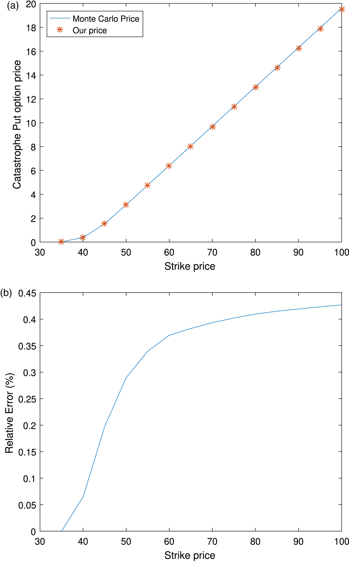
The comparison of the catastrophe put option prices obtained from the newly derived formula to the prices obtained using Monte-Carlo simulations is shown in Figure 1(a) for different values of the strike price  $K$. We can observe from Figure 1(a) that the derived formula gives prices that are close to the corresponding Monte-Carlo prices for all possible scenarios, namely in-the-money, out-of-the-money, and at-the-money. Furthermore, the relative difference between the two prices is demonstrated in Figure 1(b) which further validates the accuracy of our formula, the maximum relative difference being less than 0.45%. The numerical experiments also demonstrate the efficacy of our pricing formula over Monte-Carlo simulations, as the derived method only takes around 2.49 s to obtain one option price in comparison with 1115.4 s for Monte-Carlo using 500,000 sample paths. In other words, without this newly derived formula, one would need to wait approximately 450 times to obtain the price of a catastrophe option.

Figure 1. The comparison on catastrophe put option prices calculated with our formula and those obtained through Monte-Carlo simulation. (a) Monte-Carlo price versus our price. (b) The relative difference between Monte-Carlo price and our price.
5. Conclusion
In this paper, a closed-form pricing formula for pricing European catastrophe equity put option is derived. The newly derived closed-form formula is independent of the model (up to the existence of the joint characteristic function of the underlying asset and the loss process) for underlying asset and totally avoids the need for solving several layers of infinite sums, as most previous approaches required. The application of the proposed pricing formula is presented for two modeling frameworks when the underlying stock is governed by a jump-diffusion process and risk-free interest rate follows a stochastic process. The advantage of adopting the newly derived formula in pricing is demonstrated through numerical experiments.
6. Conflicts of interest
The authors declare no conflict of interest.
Appendix A
Proof From Theorem 5 in Shephard [Reference Shephard12], we have the following relationship between the joint cumulative distribution function (CDF)  $F(x,y)$ and the joint characteristic function
  $\phi (t_1,t_2)$ of a two-dimensional random variable
  $(X,Y)$,
 \begin{equation} 4F(x,y)-2(F_{X}(x)+F_Y(y))+1=\frac{1}{\pi^2}\int_0^{\infty}\int_0^{\infty} \Delta_{t_1}\Delta_{t_2}\left[\frac{\phi(t_1,t_2)e^{{-}it_1x-it_2y}}{it_1it_2}\right]dt_1\,dt_2, \end{equation}
where  $F_X(\cdot ), F_Y(\cdot )$ denote the marginal CDF of
  $X$ and
  $Y$ respectively. Furthermore, for a single random variable
  $X$,
$X$,  $Y$, we can write the following relationship,
 \begin{align} F_X(x)& =\frac{1}{2}-\frac{1}{2\pi}\int_0^{\infty} \Delta_{t_1}\left[\frac{\phi(t_1,0)\,e^{{-}it_1x}}{it_1}\right]dt_1, \end{align}
 \begin{align} F_Y(y)& =\frac{1}{2}-\frac{1}{2\pi}\int_0^{\infty} \Delta_{t_2}\left[\frac{\phi(0,t_2)\,e^{{-}it_2y}}{it_2}\right]dt_2. \end{align}
 Consider the expectation  $E(e^X)$ which is given by
 \begin{equation} E(e^X)=\int_{-\infty}^{\infty}\int_{-\infty}^{\infty}e^xf(x,y)\,dx\,dy=\phi({-}i,0). \end{equation}
 One can observe from Eq. (A.4) that  ${e^xf(x,y)}/{\phi (-i,0)}$ is a probability density function (PDF) of a two-dimensional random variable, say
  $(\tilde {X},\tilde {Y})$. Let
  $\tilde {F}(x,y)$ and
  $\tilde {\phi }(t_1,t_2)$ denote the joint CDF and the joint characteristic function of
  $(\tilde {X},\tilde {Y})$. Then,
 \begin{equation} E(e^XI_{\{X\leq x, Y\leq y\}})=\int_{-\infty}^{y}\int_{-\infty}^{x}e^xf(x,y)\,dx\,dy=\phi({-}i,0)\tilde{F}(x,y). \end{equation}
 Now, the joint characteristic function of  $(\tilde {X},\tilde {Y})$ can be derived as
 \begin{align*} \tilde{\phi}(t_1,t_2)& =E(e^{it_1\tilde{X}+it_2\tilde{Y}})\\ & =\int_{-\infty}^{\infty}\int_{-\infty}^{\infty}e^{it_1x+it_2y}\frac{e^xf(x,y)}{\phi({-}i,0)}\,dx\,dy\\ & =\frac{\phi(t_1-i,t_2)}{\phi({-}i,0)}. \end{align*}
Substituting Eqs. (A.1) to (A.3) in Eq. (A.5) leads to
 \begin{align} E(e^XI_{\{X\leq x, Y\leq y\}})& =\phi({-}i,0)\tilde{F}(x,y)\nonumber\\ & =\frac{\phi({-}i,0)}{4}\left[1+\frac{1}{\pi^2}\int_0^{\infty}\int_0^{\infty} \Delta_{t_1}\Delta_{t_2}\left[\frac{\phi(t_1-i,t_2)\,e^{{-}it_1x-it_2y}}{\phi({-}i,0)it_1it_2}\right]dt_1\,dt_2 \right.\nonumber\\ & \quad -\frac{1}{\pi}\int_0^{\infty} \Delta_{t_1}\left[\frac{\phi(t_1-i,0)\,e^{{-}it_1x}}{\phi({-}i,0)it_1}\right]dt_1\nonumber\\ & \quad \left.-\frac{1}{\pi}\int_0^{\infty} \Delta_{t_2}\left[\frac{\phi({-}i,t_2)e^{{-}it_2y}}{\phi({-}i,0)it_2}\right]dt_2\right] \end{align}
 Let  $F(x,y)=P(Y_T\leq x, -L_T\leq y)$,
  $f(x,y)$, and
  $\phi (t_1,t_2)=E(e^{it_1Y_T+it_2(-L_T)})$ denote the CDF, PDF, and the characteristic function of
  $(Y_T,-L_T)$, respectively. Using Eqs. (A.1) to (A.6), the results (7) and (8) follow. □