


1 Introduction
This is the second of a series of investigations of the mean flow within a turbulent boundary layer near a stationary plane that bounds a fluid having an axisymmetric circumferential velocity  $v_{\infty }(r)$, where
  $r$ is the cylindrical radius. Loper (Reference Loper2020; referred to as Part 1) investigated the boundary-layer flow beneath a fluid in rigid-body rotation, with
  $v_{\infty }\sim r$; that investigation is the turbulent analogue of the Bödewadt problem (Bödewadt (Reference Bödewadt1940); see § XI.1 (pp. 213–218) of Schlichting (Reference Schlichting1968)). Here in Part 2 the outer flow is generalized to a power law with
  $v_{\infty }\sim r^{2\unicode[STIX]{x1D703}-1}$, with the parameter
  $\unicode[STIX]{x1D703}$ treated as a constant.
This investigation is motivated by a desire to gain a better understanding of the mean flow near the ground in atmospheric vortices, particularly tornadoes, with an emphasis on eye formation. In order to provide orientation, the following subsection discusses the boundary-layer behaviour beneath a swirling flow, as it pertains to the formation of an eye.

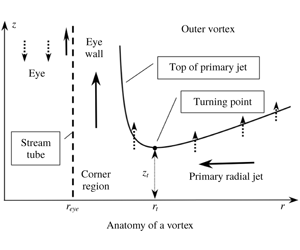
Figure 1. The anatomy of a vortex in the meridional ( $r,z$) plane. The dashed line vertical is the stream tube bounding the eye and the point (
 $r_{eye},0$) is a separation point. The solid curve is the upper boundary of the primary jet; this jet is narrowest at the turning point (
 $r_{t},z_{t}$), denoted by the black dot. Solid arrows denote strong (unit order) speeds and dotted arrows denote smaller-order speeds. Air flows radially inward within the primary jet, turns upward within the corner region and flows up within the eyewall.
1.1 Boundary-layer breakdown and eye formation
Broadly speaking there are two types of rotating storms, exemplified by tropical cyclones and tornadoes. The former are long lived (many days), are strongly affected by the Coriolis force and have small aspect ratio (height to width), while the latter are short lived (typically less than an hour), are not directly affected by the Coriolis force and have large aspect ratio. A typical and striking feature of these storms is their double-cell structure, with a relatively quiescent central eye, having radius  $r_{eye}$, that is surrounded by a swirling flow, as illustrated in figure 1. The swirling flow consists of an outer vortex separated from the eye by an eyewall and separated from the ground by a turbulent boundary layer. The eyewall and boundary layer intersect in the corner region.
A key question is: why does a rotating storm develop an eye? This question has been the subject of several studies focusing on tropical cyclones (e.g. Smith Reference Smith1980, Reference Smith2005; Pearce Reference Pearce2005; Oruba, Davidson & Dormy Reference Oruba, Davidson and Dormy2017; Oruba, Davidson, & Dormy Reference Oruba, Davidson and Dormy2018), but the reason why tornadoes have eyes has received little attention. A pioneering study by Eliassen (Reference Eliassen1971) sought to answer this question by considering a model of turbulent boundary-layer flow that includes the slip boundary condition. Upon expanding the velocities in powers of radius, he found that at dominant order no turbulent boundary layer is possible and concluded that close to the axis the flow must be rigid-body rotation with no vertical flow. This analysis is both mathematically and physically suspect. On the mathematical side, the slip condition is valid provided that the Reynolds number based on the velocity difference across the boundary layer is large. But with rigid-body rotation, this velocity difference tends to zero as  $r\rightarrow 0$, so that the assumption of turbulent flow and the application of the slip condition is inappropriate in this limit. In other words, the boundary-layer problem with the slip condition is ill-posed in the limit
  $r\rightarrow 0$; a generalized boundary condition including both the slip and no-slip formalisms should be employed. On physical grounds, Eliassen’s result implies that a boundary layer cannot exist and no vertical flow is possible on the axis of a vortex, which is clearly an unrealistic conclusion. Further, if Eliassen’s argument were correct, then all rotating storms would have eyes. But this is not the case; storms having relatively weak swirl lack eyes.
Nevertheless, Eliassen’s basic finding – that boundary-layer dynamics controls the location of the eye – is confirmed and quantified in the present study. However, an important difference is that control is provided by the boundary-layer structure outside the corner region, rather than inside. In the boundary-layer formulation, with radial viscous terms ignored, a boundary condition on the radial inflow at the eye radius cannot be satisfied. It follows that formation of an eye and corner region must be an inherent feature of boundary-layer dynamics that arises spontaneously. This leads to a modification of the question: why does the boundary layer beneath a vortex spontaneously break down?
To understand the structural implication of eye formation, it is helpful to contrast the topological structure of axisymmetric flows without and with eyes. It has been found in Part 1 that if the circumferential outer flow is rigid-body motion, meridional flow consists of radial inflow (predominantly within the primary jet close to the ground; see § I.1.1 of Part 1) and a compensatory upward flow. (Sections, equations, tables and figures in Loper (Reference Loper2020) are preceded by ‘I.’.) The radial influx within the primary jet is a function of  $r$ that tends smoothly to zero as
  $r\rightarrow 0$; there is no eye and the corner region (where the boundary-layer formulation breaks down) has a very small radial extent abutting
  $r=0$; see § I.3.2.1. When the circumferential flow above the boundary layer varies more generally with
  $r$ and the vortex has an eye, the topology of the meridional flow must change; it must have a stream tube (that is, a cylindrical surface of revolution) separating the eye region from the vortex and radial flux within the primary jet must go to zero as
  $r\rightarrow r_{eye}$, not as
  $r\rightarrow 0$. Within the boundary-layer formulation, with radial derivatives ignored, there is no flexibility to satisfy such a condition; it can be satisfied only by re-instating the radial derivatives in the momentum equation. These added terms are effective within the corner region. When the vortex has an eye, the corner region no longer abuts
  $r=0$, but must occur at finite radius as illustrated in figure 1.
Clues to the answer lie in the boundary-layer problem formulated in Part 1. This problem contains two dimensionless parameters:  $\unicode[STIX]{x1D703}$, defined by (I.3.9) and (2.9), which describes the radial structure of the swirling outer flow, and
  $\unicode[STIX]{x1D70C}$, defined by (I.3.2) and (2.4), which both quantifies the effect of a rough boundary and acts as dimensionless radial coordinate. Consider first the control of boundary-layer behaviour provided by
  $\unicode[STIX]{x1D703}$. It is shown in Part 1 that for rigid-body outer flow (having
  $\unicode[STIX]{x1D703}=1$), the boundary layer is well-behaved and no eye occurs. At the other extreme, for a potential vortex (having
  $\unicode[STIX]{x1D703}=0$), the boundary-layer problem is singular and has no solution; see § I.3.2. It follows logically that, as
  $\unicode[STIX]{x1D703}$ decreases, the boundary-layer formulation progressively breaks down and eventually a boundary layer can no longer exist.
This simple conceptual picture is modified – and mapped into physical space – by the influence of the second parameter  $\unicode[STIX]{x1D70C}$. It is evident from the physical structure of vortex flows with eyes that the boundary layer is well behaved if
  $\unicode[STIX]{x1D70C}$ is sufficiently large and that the boundary layer breaks down when
  $\unicode[STIX]{x1D70C}$ becomes small. The parameter
  $\unicode[STIX]{x1D70C}$ quantifies the geometric strengthening of radial flow within the primary jet, the compensatory increase of axial outflow from the boundary layer as the radius decreases and the associated increase in inertial oscillations. The strengthening of radial flow is illustrated (for
  $\unicode[STIX]{x1D703}=1.0$) in figure I.8, which displays graphs of the radial velocity component versus axial distance for four values of
  $\unicode[STIX]{x1D70C}$; as radius decreases, the magnitudes of the radial speed and its axial oscillations increase. Similarly, the strengthening of axial flow and oscillations with decreasing radius is seen in figure I.10. The increase in the strength of meridional-plane oscillations with decreasing radius is illustrated in the set of hodographs found in figure I.11.
It is likely that the breakdown of the boundary-layer formulation is associated with the increase in strength of inertial forces, relative to the viscous forces, with decreasing radius. This increase is seen in the magnitudes of the radial jets, which are an integral part of the meridional-plane oscillations (see figure 11). Recall that radial flow consists of a sequence of jets: a primary jet of radial inflow close to the ground, a weaker secondary jet of radial outflow immediately above, etc. Air is fed into the secondary radial jet by a positive axial flow from the primary jet with parcels of air moving upward and away from the axis of rotation. This flow requires a positive radial acceleration near the boundary between these two jets. As these jets increase in strength with a decrease in radius, barring an increase in the axial extent of the jets, the requisite radial acceleration must increase. Boundary-layer instability leading to the formation of the eyewall may arise from an inability to provide this acceleration, so that the outflow from the primary jet is directed upward into the eyewall rather radially outward within the secondary jet.
As the meridional-plane oscillations increase in strength, it becomes increasingly difficult to obtain converged solutions to the boundary-layer problem using the spectral/iterative procedure described in appendix I.B – an indication that the boundary-layer flow is becoming unstable. The averaging procedure described in appendix I.B.7.3 is a powerful tool in obtaining converged solutions – so powerful that it permits the procedure to obtain solutions that are actually unstable. That is, for a given value of  $\unicode[STIX]{x1D703}$, a critical value of
  $\unicode[STIX]{x1D70C}$, denoted by subscript
  $c$, can be identified such that solutions of the boundary-layer problem are stable for
  $\unicode[STIX]{x1D70C}>\unicode[STIX]{x1D70C}_{c}$ and unstable for
  $\unicode[STIX]{x1D70C}<\unicode[STIX]{x1D70C}_{c}$.
In order to track boundary-layer breakdown, it is helpful to identify a specific physical and mathematical point associated with this process. As the radial influx within the primary jet turns upward within the corner region to form the eyewall, the upper boundary of this jet must increase in height, as illustrated in figure 1. This requires the slope of the primary jet, which is positive at large radius, to change sign at the turning point, where this jet is narrowest. Since boundary-layer breakdown increases as  $\unicode[STIX]{x1D703}$ decreases, the locus of turning-point values in the
  $\unicode[STIX]{x1D70C},\unicode[STIX]{x1D703}$ plane has a negative slope, as illustrated by the solid line in figure 2. In the following, the radial and axial locations of the turning point are denoted by
  $r_{t}$ and
  $z_{t}$. Presumably
  $r_{t}$ gives a sense of the radial location of the eyewall and corner region and
  $z_{t}$ gives a sense of the width and height of the corner region. The following analysis seeks to provide a firmer foundation for this conjectured scenario of boundary-layer structure near the corner region.

Figure 2. Parameter regime diagram (not to scale). The parameter  $\unicode[STIX]{x1D70C}$ quantifies the effect of boundary roughness;
  $\unicode[STIX]{x1D703}$ quantifies swirl of the outer flow. The sloping solid line is a schematic of the turning-point curve; this is shown accurately in figure 15. The stippled area indicates the region in which the boundary-layer solution is inaccurate and radial viscous forces and vertical acceleration become important. The solution corresponding to the dot at
  $\unicode[STIX]{x1D70C}=0$ and
  $\unicode[STIX]{x1D703}=1$ is found in § I.5. The vertical dashed lines correspond to the detailed solutions found in §§ I.6 and 4. The boxed numbers I.1, 1, 2 and 3 indicate the associated data tables in Part 1 and in the Appendix.
1.2 Organization
This paper is organized as follows. The flow problem, non-dimensionalization and diffusivity models developed in Part 1 are summarized in § 2. Solutions of the boundary-layer problem with axially uniform flow resistance (model A) are summarized in table 1 and illustrated and discussed in § 3; solutions are found only for  $\unicode[STIX]{x1D703}>0.55$, which severely limits the utility of model A. Model B, having variable resistance, performs much better and produces solutions that appear to be realistic. A representative set of solutions using model B with
  $\unicode[STIX]{x1D703}=0.2$ is summarized in table 2 and illustrated and discussed in § 4. The conjecture about eye formation presented immediately above is bolstered in this section; it is found that the primary jet has a minimum thickness
  $z_{t}$ at a finite radius
  $r_{t}$, with the jet thickening and strengthening as radius decreases further. The location of the turning point depends on
  $\unicode[STIX]{x1D703}$, as do the velocity magnitudes and gradients at
  $r_{t}$; these variations with
  $\unicode[STIX]{x1D703}$ are quantified in § 5. The analysis and results are summarized in § 6, with § 7 containing some concluding remarks. Solutions obtained using the spectral/iterative procedure described in appendix I.B are summarized in a set of three tables found in the Appendix.
2 The problem
This section summarizes the mathematical problem, developed in Part 1, governing the mean turbulent flow within the boundary layer adjacent to a rough stationary plane bounding a fluid having general axisymmetric circumferential (swirling) flow. The boundary-layer problem, presented in § I.2, consists of three partial differential equations: two transverse momentum equations and the continuity equation (I.2.3)–(I.2.5), together with suitable boundary conditions; these equations govern the variation of the radial, circumferential and axial velocity components ( $u$,
$u$,  $v$ and
  $w$, respectively) as functions of
  $r$ and
  $z$. The eddy diffusivity is expressed as the product of the circumferential speed
  $v_{\infty }(r)$ and a diffusivity function (see (I.2.8))
 $$\begin{eqnarray}\unicode[STIX]{x1D708}(r,z)=v_{\infty }(r)L(r,z),\end{eqnarray}$$
 where  $L$ is specified by the diffusivity model; see § 2.1.
These partial differential equations are non-dimensionalized using the transformation
 $$\begin{eqnarray}\{u(r,z),v(r,z),w(r,z)\}=v_{\infty }\{F,G,\unicode[STIX]{x1D716}H^{\star }\}\end{eqnarray}$$
with
 $$\begin{eqnarray}H^{\star }=\frac{1}{\sqrt{\unicode[STIX]{x1D70C}}}H_{A}=\frac{1}{\sqrt{\unicode[STIX]{x1D70C}}}\left(H+\frac{1}{2}\unicode[STIX]{x1D701}F\right),\end{eqnarray}$$
 where  $F$,
$F$,  $G$,
$G$,  $H$,
$H$,  $H_{A}$ and
  $H^{\star }$ are functions of the variables
 $$\begin{eqnarray}\unicode[STIX]{x1D70C}=\unicode[STIX]{x1D716}r/z_{0}\end{eqnarray}$$
and
 $$\begin{eqnarray}\unicode[STIX]{x1D701}(r,z)=\frac{z}{z_{0}\sqrt{\unicode[STIX]{x1D70C}}}=\frac{z^{\star }}{\sqrt{\unicode[STIX]{x1D70C}}}.\end{eqnarray}$$
 The small dimensionless parameter  $\unicode[STIX]{x1D716}$ is related to the inverse of the local Reynolds number within the turbulent layer; see equation (I.4.5).
The transverse momentum equations are combined into a single complex equation, leading to the set of equations (I.3.7) and (I.3.13)
 $$\begin{eqnarray}H_{\unicode[STIX]{x1D701}}+\left(2\unicode[STIX]{x1D703}+{\textstyle \frac{1}{2}}\right)F+\unicode[STIX]{x1D70C}F_{\unicode[STIX]{x1D70C}}=0\end{eqnarray}$$
and
 $$\begin{eqnarray}\left(\unicode[STIX]{x1D6EC}\boldsymbol{V}_{\unicode[STIX]{x1D701}}\right)_{\unicode[STIX]{x1D701}}-H\boldsymbol{V}_{\unicode[STIX]{x1D701}}-\unicode[STIX]{x1D70C}F\boldsymbol{V}_{\unicode[STIX]{x1D70C}}+2(1-\unicode[STIX]{x1D703})F\boldsymbol{V}+\boldsymbol{i}\boldsymbol{V}^{2}=\boldsymbol{i},\end{eqnarray}$$
where
 $$\begin{eqnarray}\boldsymbol{V}=G+\boldsymbol{i}F\end{eqnarray}$$
is the complex transverse velocity,
 $$\begin{eqnarray}\unicode[STIX]{x1D703}(r)=\frac{1}{2v_{\infty }}\frac{\text{d}\left(rv_{\infty }\right)}{\text{d}r}\end{eqnarray}$$
is the non-dimensionalized vorticity of the outer fluid (see (I.3.9)) and
 $$\begin{eqnarray}\unicode[STIX]{x1D6EC}(\unicode[STIX]{x1D70C},\unicode[STIX]{x1D701})=\frac{1}{\unicode[STIX]{x1D716}z_{0}}L\left(z_{0}\unicode[STIX]{x1D70C}/\unicode[STIX]{x1D716},z_{0}\sqrt{\unicode[STIX]{x1D70C}}\unicode[STIX]{x1D701}\right)\end{eqnarray}$$
 is a dimensionless version of the diffusivity function  $L(r,z)$ (see (I.3.10)). Note that here and in the following, complex quantities (including the imaginary unit
  $\boldsymbol{i}$) are expressed using bold italic letters. Note also that
  $\unicode[STIX]{x1D703}=1$ for rigid-body motion and 0 for a potential vortex.
Equations (2.6) and (2.7) are to be solved on the interval  $0<\unicode[STIX]{x1D701}<\infty$ subject to conditions (I.3.14)
 $$\begin{eqnarray}\boldsymbol{V}(\unicode[STIX]{x1D70C},0)=H(\unicode[STIX]{x1D70C},0)=\boldsymbol{V}(\unicode[STIX]{x1D70C},\infty )-1=0.\end{eqnarray}$$
2.1 Diffusivity models
The formulation contains a function,  $L(r,z)$, that quantifies the variation of the turbulent kinematic diffusivity with axial distance. The boundary-layer problem is solved employing two simple models of this function. In model A,
  $L$ is constant, while in model B it is constant within a layer (referred to as the rough layer) that extends a distance
  $z_{0}$ from the boundary at
  $z=0$ and varies linearly with axial distance outside this layer. Linear variation of flow resistance with axial distance above the layer is based on Prandtl’s mixing-length theory (e.g. see formula (19.9) of Schlichting (Reference Schlichting1968) and § 23.5.2 of Loper (Reference Loper2017)) and is consistent with Bak’s idea that the mean shearing motions within the boundary layer are at the margin of stability (Bak Reference Bak1996).
Model A assumes that
 $$\begin{eqnarray}L=\unicode[STIX]{x1D716}z_{0}.\end{eqnarray}$$
It is readily seen that (2.10) simplifies to
 $$\begin{eqnarray}\unicode[STIX]{x1D6EC}=1.\end{eqnarray}$$
Model B assumes that
 $$\begin{eqnarray}L=\unicode[STIX]{x1D716}\left\{\begin{array}{@{}ll@{}}z_{0}\quad & \text{if}~0<z\leqslant z_{0}\\ z\quad & \text{if}~z_{0}<z.\end{array}\right.\end{eqnarray}$$
Substituting (2.14) into (2.10) yields
 $$\begin{eqnarray}\unicode[STIX]{x1D6EC}=\left\{\begin{array}{@{}ll@{}}1\quad & \text{if}~0<\unicode[STIX]{x1D701}\leqslant 1/\sqrt{\unicode[STIX]{x1D70C}}\\ \unicode[STIX]{x1D701}\sqrt{\unicode[STIX]{x1D70C}}\quad & \text{if}~1/\sqrt{\unicode[STIX]{x1D70C}}<\unicode[STIX]{x1D701}.\end{array}\right.\end{eqnarray}$$
 The parameter  $\unicode[STIX]{x1D70C}=\unicode[STIX]{x1D716}r/z_{0}$
(i) serves as a non-dimensionalized radial coordinate;
(ii) encapsulates the effects of the small parameter
 $\unicode[STIX]{x1D716}$; and
(iii) quantifies the relative importance of boundary roughness
$z_{0}$ at a given radial location.


It is estimated in § I.4.2 that a plausible range of  $\unicode[STIX]{x1D70C}$ for a tornado is
  $0.01\leqslant \unicode[STIX]{x1D70C}\leqslant 100.0$.
2.2 Discussion and orientation
The problem occurs in two versions depending on the diffusivity model chosen (model A or B) and contains one (in model A) or two (in model B) dimensionless parameters:  $\unicode[STIX]{x1D703}$ quantifying the effect of the outer-flow swirl and
  $\unicode[STIX]{x1D70C}$ quantifying the effect of the rough layer close to the ground. As explained in § I.4.2.1, the formulation with model B, which includes a diffusivity that grows linearly with axial distance outside the rough layer, is consistent with the imposition of the no-slip condition provided the rough layer has finite thickness. The rough layer is a macroscopic rendering of the surface irregularities that are parameterized by the traditional slip condition.
Depending on the prescribed value of  $z_{0}$, at a given radial location
  $r$ the parameter
  $\unicode[STIX]{x1D70C}=\unicode[STIX]{x1D716}r/z_{0}$ can range from 0 (the rough layer is infinitely thick) to
  $\infty$ (a smooth boundary). Note that the importance of boundary roughness increases as the radial distance from the axis of the vortex decreases. In the limit
  $\unicode[STIX]{x1D70C}\rightarrow 0$ the mathematical problem using model B approaches that using model A, but the physical interpretations of the results differ. That is, while results obtained with model A are valid for all values of
  $\unicode[STIX]{x1D70C}$, in the limit
  $\unicode[STIX]{x1D70C}\rightarrow 0$ results obtained with model B are valid only at the axis of symmetry. The influence of
  $\unicode[STIX]{x1D70C}$ is seen in the geometrical form of the boundary layer. The nearly linear variation of thickness with radius seen in figure I.4 is a robust feature, persisting for all values of
  $\unicode[STIX]{x1D703}$, provided
  $\unicode[STIX]{x1D70C}$ is not too small. The boundary-layer thickness is much greater than
  $z_{0}$ far from the axis of rotation, but the two have similar magnitudes when
  $\unicode[STIX]{x1D70C}=O(1)$.
The boundary-layer shape and structure are independent of the magnitude of the outer swirl,  $v_{\infty }(r)$, depending only on its radial structure through the parameter
  $\unicode[STIX]{x1D703}$ defined by (2.9). As noted in § I.3.2,
  $\unicode[STIX]{x1D703}$ is a measure of the angular-momentum gradient of the outer flow (see (I.3.15)) and as such quantifies the dynamical stiffness of the outer fluid. It has a lower limit of
  $0$; beyond that, the angular momentum of the fluid decreases with increasing radius – a configuration that is dynamically unstable. As
  $\unicode[STIX]{x1D703}$ increases in value from
  $0$, the outer fluid becomes progressively more resistant to radial motion and the boundary layer becomes correspondingly thinner. Physical reasoning does not place an upper bound on the value of
  $\unicode[STIX]{x1D703}$. In the following, attention will be limited to flow outside the eye of an atmospheric vortex, wherein
  $0<\unicode[STIX]{x1D703}<1$. (Super-rigid-body rotation having
  $\unicode[STIX]{x1D703}>1$ is expected to occur within the eye and eyewall.)
The boundary-layer equation (2.7) describes a balance between viscous and inertial forces. With  $\unicode[STIX]{x1D703}>0$, perturbations of the outer flow described by this equation occur as inertial oscillations that have axial structure. One manifestation of these oscillations is a sequence of radial jets having alternating orientations. The viscous force acts to damp these oscillations, giving a boundary layer in which the velocity perturbations decay with axial distance. The structure of this axial oscillation and decay depends on the axial structure of the diffusivity function
  $L$, as well as the parameters
  $\unicode[STIX]{x1D70C}$ and
  $\unicode[STIX]{x1D703}$. It will be seen in § 3 that if
  $L$ is constant (as in model A), solutions to the boundary-layer problem can be found only if
  $0.55<\unicode[STIX]{x1D703}$, whereas if
  $L$ increases with axial distance (as in model B), solutions can be found for a much greater range of
  $\unicode[STIX]{x1D703}$.
The structure of the boundary layer beneath a rigid-body outer flow (having  $\unicode[STIX]{x1D703}=1$) is presented in Part 1. In particular, the solution for
  $\unicode[STIX]{x1D703}=1$ using model A is described in § I.5, while the solution for
  $\unicode[STIX]{x1D703}=1$ using model B is summarized in table I.1 and described in § I.6. Those solutions are generalized here in Part 2 to the case of arbitrary power-law swirl, with
  $\unicode[STIX]{x1D703}$ constant. Wurman & Gill ((Reference Wurman and Gill2000); see also Wurman & Alexander (Reference Wurman and Alexander2005), Mallen, Montgomery & Wang (Reference Mallen, Montgomery and Wang2005) and Bĕlík et al. (Reference Bĕlík, Dokken, Schloz and Shvartsman2014)) estimated that a plausible range is
  $0.15<\unicode[STIX]{x1D703}<0.25$ for the circumferential flow outside the eye of a tornado. With this in mind, in the following analysis and discussion, the structure of the boundary layer in the case
  $\unicode[STIX]{x1D703}=0.2$ (that is,
  $v_{\infty }\sim r^{-0.6}$) will be investigated in detail in § 4, while key features of the layer will be investigated for other values of
  $\unicode[STIX]{x1D703}$ in a summary fashion in § 5.
2.2.1 Regime diagram
A guide to the ensuing calculations is provided in figure 2, which is a diagram of the regime plane. In this diagram, the vertical axis denotes variation of  $\unicode[STIX]{x1D70C}$ from 0 (bottom) to
  $\infty$ (top), while the horizontal axis denotes variation of
  $\unicode[STIX]{x1D703}$ from
  $0$ (left) to 1 (right). Model A is applicable to the horizontal line at the bottom of the diagram (at
  $\unicode[STIX]{x1D70C}=0$), while model B covers the interior of the regime plane.
The sloping line in figure 2 is a schematic representation of the turning-point curve,  $\unicode[STIX]{x1D70C}_{t}(\unicode[STIX]{x1D703})$, where the primary jet ceases to narrow with decreasing radius. Accurate representations of this curve is shown in figure 15. The stippled area in figure 2 indicates the region in which the boundary-layer solution is inaccurate, because the condition
  $w\ll v_{\infty }$ is not satisfied. The upper boundary of this region depends on the magnitude of
  $\unicode[STIX]{x1D716}$ and may well extend to the turning-point curve.
The problem using model B abounds with singularities, as follows.
(i) In the limit
$\unicode[STIX]{x1D703}\rightarrow 0$, the outer flow is a potential vortex and the boundary-layer problem has no solution.(ii) In the limit
$\unicode[STIX]{x1D703}\rightarrow \infty$, the boundary-layer thickness tends to zero as $\unicode[STIX]{x1D703}^{-1/4}$.(iii) In the limit
$\unicode[STIX]{x1D70C}\rightarrow \infty$, internal resistance to flow disappears and the no-slip condition cannot be satisfied; resistance should be parameterized by a slip condition at the boundary.(iv) The formulation has an algebraic singularity, with
$z^{\star }\sim \sqrt{\unicode[STIX]{x1D70C}}$ and $w\sim 1/\sqrt{\unicode[STIX]{x1D70C}}$, so that in the limit $\unicode[STIX]{x1D70C}\rightarrow 0$ the boundary-layer thickness tends to zero, transverse-velocity gradients tend to $\infty$ and the axial velocity from the layer tends to $\infty$. However, when $\unicode[STIX]{x1D703}\lesssim 0.42$, the boundary-layer formulation breaks down at a finite value of $\unicode[STIX]{x1D70C}$, rendering this algebraic singularity moot.


2.3 Solution procedure and format of results
The regime diagram is sampled as indicated by the horizontal axis and two dashed lines in figure 2. Specifically solutions to the problem formulated in § 2 using model A (indicated by the horizontal axis in figure 2) are summarized in table 1 found in the Appendix and are analysed and discussed in § 3. Solutions using model B are investigated in detail for two values of  $\unicode[STIX]{x1D703}$; solutions for
  $\unicode[STIX]{x1D703}=1$ are summarized in table I.1 and discussed in § I.6, while solutions for
  $\unicode[STIX]{x1D703}=0.2$ are summarized in table 2 of the Appendix and are analysed and discussed in § 4. The investigation has an arbitrary upper limit of
  $\unicode[STIX]{x1D70C}=100.0$, based on the physical reasoning found in § I.4.2. The lower limit on
  $\unicode[STIX]{x1D70C}$ is determined by the behaviour of the mathematical problem and its solutions.
The data tables found in the Appendix are organized as follows.
2.3.1 Table 1: model A
Table 1, which is discussed in § 3, summarizes solutions to the boundary-layer problem using model A, with  $\unicode[STIX]{x1D703}$ being the controlling variable; solutions are found for
  $0.55\leqslant \unicode[STIX]{x1D703}\leqslant 1$. With
  $\unicode[STIX]{x1D703}$ being a specified constant and using model A, non-dimensionalization presented in § 2 is in fact a similarity transform and the solutions are independent of
  $\unicode[STIX]{x1D70C}$. This table summarizes the values of
(i) the axial location of the tops of the primary and secondary radial jets
$\unicode[STIX]{x1D701}_{1}$ and $\unicode[STIX]{x1D701}_{2}$;(ii) the extremes of
$F$ and $G$ and their axial locations $\unicode[STIX]{x1D701}_{F}$ and $\unicode[STIX]{x1D701}_{G}$;(iii) the asymptotic and maximum normal flows
$H_{\infty }$ and $H_{max}$; and(iv) the real and imaginary parts of
$\boldsymbol{V}_{0}^{\prime }$ at $\unicode[STIX]{x1D701}=0$.


The values given in this table are visualized in figures 3 and 4.
2.3.2 Table 2: model B with $\unicode[STIX]{x1D703}=0.2$

Table 2, which is discussed in § 4, summarizes solutions to the boundary-layer problem using model B with  $\unicode[STIX]{x1D703}=0.2$; now
  $\unicode[STIX]{x1D70C}$ is the controlling variable (Using model B, the diffusivity function is a function of
  $z$; the non-dimensionalization is not a similarity transform and the solution depends on
  $\unicode[STIX]{x1D70C}$). Solutions are found for
  $0.29<\unicode[STIX]{x1D70C}<100$, with the lower bound being a practical limit; it is progressively more difficult to find converged solutions as
  $\unicode[STIX]{x1D70C}$ decreases. Specifically this table summarizes the values of
(i) the axial location of the tops of the primary and secondary radial jets
$z_{1}^{\star }$ and $z_{2}^{\star }$;(ii) the extremes of
$F$ and $G$ and their axial locations $z_{F}^{\star }$ and $z_{G}^{\star }$;(iii) the asymptotic and maximum axial flows
$H_{\infty }^{\star }$ and $H_{max}^{\star }$; and(iv) the real and imaginary parts of
$\boldsymbol{V}_{0}^{\prime }$ at $z^{\star }=0$.


These values are graphed versus  $\unicode[STIX]{x1D70C}$ in figures 7–10. With
  $z_{0}$ constant,
  $\unicode[STIX]{x1D70C}$ is the dimensionless radius and these figures visualize the boundary-layer shape and behaviour as a function of radius. Each of these figures consists of two panels, with graphs in the right-hand panels extending from
  $\unicode[STIX]{x1D70C}=0$ to 100 and those the left-hand panels extending from
  $\unicode[STIX]{x1D70C}=0$ to 1.0, in order to show more clearly the structure close to the axis of rotation.
The axial locations  $z_{1}^{\star }$,
  $z_{2}^{\star }$,
  $z_{F}^{\star }$ and
  $z_{G}^{\star }$ vary nearly linearly with
  $\unicode[STIX]{x1D70C}$ for
  $\unicode[STIX]{x1D70C}$ large, but for
  $\unicode[STIX]{x1D70C}\approx 0.3$, each of these achieves a minimum and the axial locations increase as
  $\unicode[STIX]{x1D70C}$ decreases further. These minimum locations are indicated by bold entries in table 2. The most important of these minima is that for
  $z_{1}^{\star }$, marking the turning point of the primary jet (indicated by the dot in figure 1). Table 2 shows that primary jet has a minimum thickness of
  $9.364z_{0}$ at
  $r=0.321z_{0}/\unicode[STIX]{x1D716}$ when
  $\unicode[STIX]{x1D703}=0.2$.
2.3.3 Table 3: turning-point summary
As noted previously, an important structural feature of turbulent boundary-layer flow beneath a vortex is the turning point where the upper boundary of the primary jet is closest to the bounding plane. The location  $(\unicode[STIX]{x1D70C}_{t},z_{t}^{\star })$ of the turning point is illustrated schematically by the dot in figure 1 and accurately by the dot in figure 7 (for
  $\unicode[STIX]{x1D703}=0.2$). Table 3, which is discussed in § 5, summarizes values of
  $\unicode[STIX]{x1D70C}_{t}$ and
  $z_{t}^{\star }$, together with the flow extremes, as the value of
  $\unicode[STIX]{x1D703}$ is varied in the interval
  $0.125\leqslant \unicode[STIX]{x1D703}\leqslant 0.42$. The turning point does not exist for
  $\unicode[STIX]{x1D703}\gtrsim 0.42$. The lower value is a practical limit; it becomes progressively more difficult to locate and quantify the turning point as
  $\unicode[STIX]{x1D703}$ decreases. The function
  $\unicode[STIX]{x1D70C}_{t}(\unicode[STIX]{x1D703})$ is indicated schematically in figure 2 and graphed accurately in figure 15. The data presented in table 3 are parameterized and visualized in a sequence of figures in § 5. These simple parametric representations are an important result of this investigation.
For values of  $\unicode[STIX]{x1D703}$ and
  $\unicode[STIX]{x1D70C}$ in much of the parameter plane illustrated in figure 2, solutions to the problem (2.6)–(2.11) are readily found using the procedure described in appendix I.B. The solution converges in relatively few iterations, with no oscillations in the target functions
  $H_{\infty }$ and
  $E_{e}$ as the iteration proceeds (see § I.B.7.2). However, as
  $\unicode[STIX]{x1D70C}$ decreases (that is, as the radius decreases or the roughness layer thickens) or as
  $\unicode[STIX]{x1D703}$ decreases (that is, as the outer flow becomes more vortical), so that the corresponding point in the parameter plane approaches the stippled region in figure 2, breakdown of the boundary-layer formulation is presaged by an increase in the amplitude of axial oscillations of the velocity components. This increase in oscillation amplitude causes the number of iterations needed to achieve convergence to increase rapidly. When this occurs, the rate of convergence of the iteration procedure is significantly enhanced by employing the averaging strategy described in § I.B.7.3, but this strategy is not a panacea and it is impractical to find solutions within the stippled region of figure 2.
3 Solutions using model A
Solutions to the boundary-layer problem formulated in § 2 with model A (diffusivity independent of  $z$) have been found using the iterative procedure described in appendix I.B for
  $0.55<\unicode[STIX]{x1D703}\leqslant 1$; these are summarized in table 1. For
  $0.65\approx \unicode[STIX]{x1D703}\leqslant 1$ the iterative procedure converges relatively quickly, in 100 iterations or less. However, as
  $\unicode[STIX]{x1D703}$ is decreased further, the iteration procedure becomes less stable; the additive parameter
  $\unicode[STIX]{x1D6FE}$, introduced in equation (I.B 51), must be reduced to achieve a stable iteration and the number of iteration steps required to reach a converged solution increases rapidly. Convergence is significantly enhanced by employing the averaging strategy (see § I.B.7.3), but nevertheless it is not practically possible to find solutions for
  $\unicode[STIX]{x1D703}$ less than approximately 0.55 using the solution procedure described in appendix I.B.
The solution corresponding to the point  $\unicode[STIX]{x1D703}=1$ and
  $\unicode[STIX]{x1D70C}=0$ shown on figure 2 is summarized in § I.5; this is the turbulent analogue of the Bödewadt problem. The behaviour of the solution using model A for
  $\unicode[STIX]{x1D703}\leqslant 1$ can be illustrated by graphing the quantities listed in table 1. The thickness of the layer is illustrated in figure 3, which show the variation with
  $\unicode[STIX]{x1D703}$ of the axial locations of
(i)
$\unicode[STIX]{x1D701}_{G}$: the maximum of the circumferential velocity;(ii)
$\unicode[STIX]{x1D701}_{F}$: the minimum of the radial velocity;(iii)
$\unicode[STIX]{x1D701}_{max}$: the maximum of the normal velocity (and the first zero of $F$); and(iv)
$\unicode[STIX]{x1D701}_{min}$: the internal minimum of the normal velocity (and the second zero of $F$);


these graphs are composed using the values found in the second, third, fifth and seventh columns of table 1. The layer thickens at an increasing rate as  $\unicode[STIX]{x1D703}$ decreases.

Figure 3. Graphs of  $\unicode[STIX]{x1D701}_{F}$,
  $\unicode[STIX]{x1D701}_{G}$,
  $\unicode[STIX]{x1D701}_{max}$ and
  $\unicode[STIX]{x1D701}_{min}$ versus
  $\unicode[STIX]{x1D703}$ using model A.

Figure 4. Graphs of  $F_{min}$,
  $G_{max}$,
  $H_{min}$,
  $H_{max}$ and
  $H_{\infty }$ versus
  $\unicode[STIX]{x1D703}$ using model A.
The variation of flow strength with  $\unicode[STIX]{x1D703}$ is illustrated in figure 4 which contains graphs of the extreme values of
  $F$,
$F$,  $G$ and
  $H$. As with thickness, the magnitude of the flow and strength of the meridional oscillations increase at an accelerating rate as
  $\unicode[STIX]{x1D703}$ decreases.
The structure of the flow is seen in figure 5 which contains graphs of the flow variables  $F$,
$F$,  $G$,
$G$,  $H$ and
  $H_{A}$ versus
  $\unicode[STIX]{x1D701}$ for
  $\unicode[STIX]{x1D703}=0.55$. The companion graphs for
  $\unicode[STIX]{x1D703}=1$ are seen in figure I.1. The major differences between the two sets of curves are the greater boundary-layer thickness and greater oscillations in the velocity components – particularly axial component – for
  $\unicode[STIX]{x1D703}=0.55$. These oscillations, which grow in magnitude as
  $\unicode[STIX]{x1D703}$ decreases, make it progressively more difficult to obtain a converged solution by the procedure described in appendix I.B. Oscillations of the transverse velocity components
  $F$ and
  $G$ are visualized in the hodograph shown in figure 6 and compared with the turbulent hodograph for
  $\unicode[STIX]{x1D703}=1$ and the laminar Bödewadt hodograph.

Figure 5. Graphs of the radial ( $F$), circumferential (
 $G$) and normal (
 $H$) velocity components versus
  $\unicode[STIX]{x1D701}$ using model A with
  $\unicode[STIX]{x1D703}=0.55$; the axial component
  $H_{A}$ (see (2.3)) is graphed as a dashed curve. The dotted horizontal line is the asymptotic value
  $H_{\infty }$. This is a companion to figure I.1, which contains graphs of these variables for
  $\unicode[STIX]{x1D703}=1$.

Figure 6. Hodograph of flow using model A with  $\unicode[STIX]{x1D703}=0.55$ shown as a solid curve. For comparison hodographs shown in figure I.3 for turbulent flow with
  $\unicode[STIX]{x1D703}=1$ and for laminar Bödewadt flow are replicated as a dashed and dotted curve, respectively.
3.1 Critique of model A
Model A has four characteristics that makes it unsuitable for studying the boundary-layer flow beneath vortical outer flows (having  $\unicode[STIX]{x1D703}<0.5$). First, the mathematical problem using model A contains a single parameter
  $\unicode[STIX]{x1D703}$; it lacks a parameter containing the radial coordinate. It follows that the non-dimensionalization dictates the boundary-layer shape: parabolic (
 $z\sim \sqrt{r}$). This model is incapable of replicating the nearly linear shape (
 $z\sim r$) that is seen in other studies (Kepert Reference Kepert2010a,Reference Kepertb; Nolan et al. Reference Nolan, Dahl, Bryan and Rotunno2017) and is observed in tornadoes. In contrast, it is shown in § I.6.2 and demonstrated in § 4 that model B readily produces solutions in which the boundary layer has a nearly linear shape. Secondly, the passive role of
  $\unicode[STIX]{x1D70C}$ does not permit transposition of mathematical results into the physical domain, making it impossible to verify the mechanism of boundary-layer breakdown postulated in § 1.1.
The third undesirable characteristic of model A is the large and persistent axial oscillations of the velocity components. An asymptotic analysis reveals that for  $\unicode[STIX]{x1D703}\ll 1$ the axial wavelength of the oscillations is
  $\unicode[STIX]{x03C0}H_{\infty }/2\sqrt{\unicode[STIX]{x1D703}}$ and the axial decay scale of the boundary layer is
  $H_{\infty }^{3}/4\unicode[STIX]{x1D703}$. If
  $H_{\infty }$ is of unit order in this limit, the axial structure is predominantly oscillatory, with a weak decay. This structure is not believed to accurately represent the turbulent boundary layer. The large oscillations and weak axial decay result from the axial uniformity of flow resistance. In contrast, in model B resistance increases with axial distance outside the rough layer and acts to suppress the amplitude of oscillations. With model B the asymptotic axial structure of the boundary layer is a damped oscillation with wavelength
  $\unicode[STIX]{x03C0}\sqrt{\unicode[STIX]{x1D70C}}/2\sqrt{\unicode[STIX]{x1D703}}$ and axial decay scale
  $\sqrt{\unicode[STIX]{x1D70C}}/4\sqrt{\unicode[STIX]{x1D703}}$.
The fourth characteristic of model A follows from the third; the large axial oscillations are difficult to accurately quantify using the solution procedure described in appendix I.B that involves a truncated Fourier sine series. An improved procedure would explicitly represent these damped oscillations, rather than relying on a sine series. But given the inherent limitations of model A, this modification is rather pointless.
To sum up, model A is difficult to implement and is incapable of producing satisfactory boundary-layer solutions for vortical outer flow. However, as demonstrated in § 4, using model B the iteration procedure readily produces reasonable results.
4 Solutions using model B with $\unicode[STIX]{x1D703}=0.2$

This section investigates the shape and structure of the turbulent boundary layer using model B for a representative value of  $\unicode[STIX]{x1D703}$: 0.2, so that
  $v_{\infty }\sim r^{-0.6}$. Model B introduces a second dimensionless parameter,
  $\unicode[STIX]{x1D70C}$, and the presentation of results is necessarily more complicated than for model A. Using the iteration procedure described in appendix I.B with
  $\unicode[STIX]{x1D703}=0.2$, solutions are found for
  $\unicode[STIX]{x1D70C}\geqslant 0.29$ and are summarized in table 2. As
  $\unicode[STIX]{x1D70C}$ decreases toward 0.29, the behaviour of the solution mirrors that of the solution using model A as
  $\unicode[STIX]{x1D703}$ decreases toward 0.55; oscillations grow in magnitude and it becomes increasingly difficult to obtain a converged solution, with the practical limit being
  $\unicode[STIX]{x1D70C}\approx 0.29$. (The solutions for
  $\unicode[STIX]{x1D70C}\leqslant 0.31$ are in fact unstable, and have been found using the averaging procedure described in appendix I.B.7.3.) In addition, a new structural feature occurs that does not occur for
  $\unicode[STIX]{x1D703}=1.0$: the turning radius,
  $\unicode[STIX]{x1D70C}_{t}$, where the primary jet is thinnest, with the jet broadening as
  $\unicode[STIX]{x1D70C}$ decreases from
  $\unicode[STIX]{x1D70C}_{t}$.

Figure 7. Graphs of the dimensionless axial locations of the tops of the primary ( $z_{1}^{\star }$) and secondary (
 $z_{2}^{\star }$) jets, the maximum (
 $z_{G}^{\star }$) of the circumferential component of velocity (
 $G$) and the minimum (
 $z_{F}^{\star }$) of the radial component of velocity (
 $F$) using model B with
  $\unicode[STIX]{x1D703}=0.2$: for
  $0<\unicode[STIX]{x1D70C}<100$ in (b) and
  $0<\unicode[STIX]{x1D70C}<1.0$ in (a). The solid curves delimit the domains of radial flow (that is, the boundaries of the primary and secondary jets), with the hollow arrows denoting the direction of flow in the meridional plane. The dots denote the turning point, where
  $z_{1}^{\star }(\unicode[STIX]{x1D70C})$, marking the top of the primary jet, is a minimum. The inset shows in more detail the structure of the primary jet near the turning point. Compare with figure I.4.
The organization of this section follows that of § I.6, focusing on graphs of the various quantities listed in table 2. Specifically, recalling the relations between calculated and physical quantities given in (I.6.1),
(i) figure 7 contains graphs of
$z_{1}^{\star }$, $z_{2}^{\star }$, $z_{G}^{\star }$ and $z_{F}^{\star }$ versus $\unicode[STIX]{x1D70C}$;(ii) figure 8 contains graphs of
$H_{\infty }^{\star }$ and $H_{max}^{\star }$ versus $\unicode[STIX]{x1D70C}$;(iii) figure 9 contains graphs of
$G_{max}$ and $F_{min}$ versus $\unicode[STIX]{x1D70C}$; and(iv) figure 10 contains graphs of
$G^{\prime }(0)/\sqrt{\unicode[STIX]{x1D70C}}$ and $F^{\prime }(0)/\sqrt{\unicode[STIX]{x1D70C}}$ versus $\unicode[STIX]{x1D70C}$.


As in § I.6, each of these figures consists of two panels, with graphs in the right-hand panels extending from  $\unicode[STIX]{x1D70C}=0$ to 100 and those in the left-hand panels extending from
  $\unicode[STIX]{x1D70C}=0$ to 1.0, in order to show more clearly the structure close to the axis of rotation. In each of figures 7–10 the vertical dotted line indicates the radial location of the turning point
  $\unicode[STIX]{x1D70C}_{t}=0.321$ for
  $\unicode[STIX]{x1D703}=0.2$. The function
  $\unicode[STIX]{x1D70C}_{t}(\unicode[STIX]{x1D703})$ is graphed for
  $0.125<\unicode[STIX]{x1D703}\cong 0.42$ in figure 15.
4.1 Boundary-layer shape
The shape of the boundary layer is illustrated in figure 7, which contains graphs of the axial locations of extremes of the velocity components versus  $\unicode[STIX]{x1D70C}$. This figure, which is a companion to figure I.4, shows that
(i) the boundary-layer thickness varies approximately linearly with
$\unicode[STIX]{x1D70C}$ for $\unicode[STIX]{x1D70C}\gtrsim 0.4$;(ii) the boundary layer for
$\unicode[STIX]{x1D703}=0.2$ is approximately twice as thick as that for $\unicode[STIX]{x1D703}=1.0$;(iii) the turning point, where the primary jet is at its thinnest, is located at
$\unicode[STIX]{x1D70C}_{t}\approx 0.321$ and $z_{t}^{\star }\approx 9.364$ for $\unicode[STIX]{x1D703}=0.2$; and(iv) for
$\unicode[STIX]{x1D70C}<\unicode[STIX]{x1D70C}_{t}$, the primary-jet thickness increases with diminishing $\unicode[STIX]{x1D70C}$.


The turning point near  $\unicode[STIX]{x1D70C}=0.321$ and the growth of the boundary-layer thickness with decreasing
  $\unicode[STIX]{x1D70C}$ for
  $\unicode[STIX]{x1D70C}<\unicode[STIX]{x1D70C}_{t}$ are novel features not seen in the solution for
  $\unicode[STIX]{x1D703}=1.0$ presented in § I.6. This point, whose existence was postulated in § 1.1 and is confirmed by figure 7, provides a valuable clue to the structure of vortices; the behaviour of
  $\unicode[STIX]{x1D70C}_{t}$ as
  $\unicode[STIX]{x1D703}$ is varied is investigated in § 5.
4.2 Velocity magnitudes
The magnitude of the flow within the boundary layer for  $\unicode[STIX]{x1D703}=0.2$ is illustrated in figures 8 and 9, with figure 8 showing the radial variation of the asymptotic and maximum axial velocities, while figure 9 shows the radial variation of the maximum value of circumferential velocity component and the minimum value of the radial velocity component.

Figure 8. Graphs of the maximum ( $H_{max}^{\star }$) and asymptotic (
 $H_{\infty }^{\star }$) dimensionless axial velocity component using model B with
  $\unicode[STIX]{x1D703}=0.2$: for
  $0<\unicode[STIX]{x1D70C}<100$ in (b) and
  $0<\unicode[STIX]{x1D70C}<1.0$ in (a). Compare with figure I.5.

Figure 9. Graphs of the maximum circumferential ( $G_{max}$) and minimum radial (
 $F_{min}$) velocity components using model B with
  $\unicode[STIX]{x1D703}=0.2$: for
  $0<\unicode[STIX]{x1D70C}<100$ in (b) and
  $0<\unicode[STIX]{x1D70C}<1.0$ in (a). Compare with figure I.6.
These figures, which are companions to figures I.5 and I.6, respectively, demonstrate that
(i) the extremes of the velocity components are relatively insensitive to the value of
$\unicode[STIX]{x1D70C}$ if $\unicode[STIX]{x1D70C}$ is significantly greater than $\unicode[STIX]{x1D70C}_{t}$;(ii) as
$\unicode[STIX]{x1D70C}$ decreases with $\unicode[STIX]{x1D70C}<\unicode[STIX]{x1D70C}_{t}$, the extremes increase in magnitude, with the increase in the magnitude of $G$ being the most modest and the increase in extremes of $H^{\star }$, particularly $H_{max}^{\star }$, being the greatest.


Noting that  $w/v_{\infty }=\unicode[STIX]{x1D716}H^{\star }$ and that the boundary-layer formulation requires
  $w\ll v_{\infty }$, it is readily seen from figure 8 that the formulation is not valid for
  $\unicode[STIX]{x1D70C}\lessapprox 0.2$ when
  $\unicode[STIX]{x1D703}=0.2$.
4.3 Gradients at the boundary
The radial variations of the circumferential and radial velocity gradients at the boundary are illustrated in figure 10. This is a companion to figure I.7. As with the velocity magnitudes, the magnitudes of these gradients are quite insensitive to the value of  $\unicode[STIX]{x1D70C}$ if
  $\unicode[STIX]{x1D70C}\gg \unicode[STIX]{x1D70C}_{t}$, but as
  $\unicode[STIX]{x1D70C}$ decreases, the circumferential gradient decreases and the radial gradient increases in magnitude. This suggests that scour produced by the winds close to the eyewall of a tornado is predominantly radially inward. Radially dominant surface stress has been inferred from an analysis of tree-fall orientations by Karstens et al. (Reference Karstens, Gallus, Lee and Finley2013), who attributed this pattern to topographic channelling of winds. The present analysis suggests that radial dominance close to the axis of rotation may be an intrinsic feature of vortical flows. Radially dominant surface stress has also been found in a large-eddy vortex simulation that explicitly resolves non-axisymmetric eddies (Nolan et al. Reference Nolan, Dahl, Bryan and Rotunno2017).

Figure 10. Graphs of the circumferential (positive values) and radial (negative values) velocity gradients at the boundary: for  $0<\unicode[STIX]{x1D70C}<100$ in (b) and
  $0<\unicode[STIX]{x1D70C}<1.0$ in (a). Compare with figure I.7.
4.4 Flow structure
The flow structure within the boundary layer with  $\unicode[STIX]{x1D703}=0.2$ is illustrated in figures 11, 12 and 13, which contain graphs of the radial (
 $F=u/v_{\infty }$), circumferential (
 $G=v/v_{\infty }$) and axial (
 $H^{\star }=\unicode[STIX]{x1D716}w/v_{\infty }$) components of velocity versus
  $z^{\star }=z/z_{0}$. These figures are companions to figures I.8, I.9 and I.10, respectively, which illustrate these velocity components with
  $\unicode[STIX]{x1D703}=1.0$. Each of these six figures consists of four panels showing profiles of the velocity components versus
  $z^{\star }$ for specified values of
  $\unicode[STIX]{x1D70C}$, with the
  $z^{\star }$ axis being vertical and the corresponding velocity component displayed horizontally. These figures illustrate the evolution of the axial profiles of the velocity components as
  $\unicode[STIX]{x1D70C}$ varies from large (at the right) to small (at the left). The corresponding values of
  $\unicode[STIX]{x1D70C}$ for the right-hand and two middle panels are the same (that is, 100.0, 10.0 and 1.0) in all six figures, while the values of
  $\unicode[STIX]{x1D70C}$ for the left-hand panel of figures I.8, I.9 and I.10 is 0.1 with the left-hand panels of figures 11, 12 and 13 containing velocity profiles close to the turning radius:
  $\unicode[STIX]{x1D70C}=0.32$.

Figure 11. Graphs of the dimensionless radial velocity,  $F$, versus
  $z^{\star }=z/z_{0}$ at the radial locations as indicated. The vertical dotted lines denote values of
  $F$ in two-tenths intervals. Note the changes in vertical scale. Compare with figure I.8.

Figure 12. Graphs of the dimensionless circumferential velocity,  $G$, versus
  $z^{\star }$ at the radial locations as indicated. The vertical dashed lines denote the asymptotic value
  $G=1.0$. Note the changes in vertical scale. Compare with figure I.9.

Figure 13. Graphs of the dimensionless axial velocity,  $H^{\star }$, versus
  $z^{\star }$ at the radial locations as indicated. The vertical dashed lines denote the asymptotic values of
  $H^{\star }$. The vertical dotted lines denote values of
  $H^{\star }$ in steps of 5.0. Note the changes in vertical scale. Compare with figure I.10.
Figures 11, 12 and 13, in comparison with figures I.8, I.9 and I.10, show that
(i) the boundary layer for
$\unicode[STIX]{x1D703}=0.2$ is much thicker than that for $\unicode[STIX]{x1D703}=1.0$, particularly for $\unicode[STIX]{x1D70C}\leqslant 1$;(ii) for
$\unicode[STIX]{x1D70C}\gg 1$, the meridional velocity components for $\unicode[STIX]{x1D703}=0.2$ and 1.0 have similar magnitude and structure but(iii) for
$\unicode[STIX]{x1D70C}\leqslant 1$, the meridional velocity components for $\unicode[STIX]{x1D703}=0.2$ are significantly larger in magnitude than those for $\unicode[STIX]{x1D703}=1.0$; and(iv) the magnitude of the meridional oscillations increases as
$\unicode[STIX]{x1D70C}$ decreases.


4.4.1 Hodograph
The hodograph of the transverse-plane flow using model B with  $\unicode[STIX]{x1D703}=0.2$ and
  $\unicode[STIX]{x1D70C}=0.32$ is shown in figure 14 as a solid curve. For comparison this figure contains the hodograph for
  $\unicode[STIX]{x1D703}=1.0$ and
  $\unicode[STIX]{x1D70C}=0.32$, graphed as a dashed curve.
These hodographs confirm that as the outer-flow swirl increases (that is, as  $\unicode[STIX]{x1D703}$ decreases) the magnitude of the meridional flow increases and the axial gradient of
  $G$ near the boundary decreases relative to that of
  $F$.
$F$.
4.5 Discussion of boundary-layer shape and structure using model B
The primary jet is a strong radial inflow near the ground, as illustrated schematically in figure 1. It has been shown in Part 1 (see figure I.4) that in the case of rigid-body outer flow ( $\unicode[STIX]{x1D703}=1$), the height,
  $z_{1}^{\star }$, of the primary jet varies nearly linearly with
  $\unicode[STIX]{x1D70C}$ and tends smoothly and monotonically to zero as
  $\unicode[STIX]{x1D70C}\rightarrow 0$, but figure 7 paints a different picture when the outer flow is vortical. In this case,
  $z_{1}^{\star }$ again varies nearly linearly with
  $\unicode[STIX]{x1D70C}$ for
  $\unicode[STIX]{x1D70C}\geqslant 0.5$, but the primary jet has a minimum thickness at a finite radius
  $\unicode[STIX]{x1D70C}_{t}$ with its thickness increasing as
  $\unicode[STIX]{x1D70C}$ continues to decrease. The minimum point on the upper boundary of the primary jet is defined as the turning point
  $(\unicode[STIX]{x1D70C}_{t},z_{t}^{\star })$.

Figure 14. Hodographs of the transverse-plane flow with  $\unicode[STIX]{x1D70C}=0.32$ and
  $\unicode[STIX]{x1D703}=0.2$ (solid curve) and 1.0 (dashed curve). Compare with figure I.11.
To understand this difference in morphology of the upper boundary of the primary jet for  $\unicode[STIX]{x1D703}=1.0$ and 0.2, consider the geometric evolution of a graph of the function of
  $z_{1}^{\star }(\unicode[STIX]{x1D70C})$ as the flow becomes more vortical (that is, as
  $\unicode[STIX]{x1D703}$ decreases from unity toward zero). This function, which is initially monotonic, develops a kink and when
  $\unicode[STIX]{x1D703}\approx 0.42$ has a zero slope at a specific radius:
  $\unicode[STIX]{x1D70C}\approx 0.17$. The thickness of the primary jet is
  $z^{\star }\approx 4.17$ when this occurs; see the first row of table 3. As the magnitude of
  $\unicode[STIX]{x1D703}$ decreases further, this critical point bifurcates into a minimum point and a maximum point, with the minimum point (the turning point) occurring at a greater value of
  $\unicode[STIX]{x1D70C}$ than the maximum point.
In addition to the thickness, there are significant variations in the structure of the boundary layer as  $\unicode[STIX]{x1D70C}$ and
  $\unicode[STIX]{x1D703}$ change. It is seen in both figures I.8–I.10 for
  $\unicode[STIX]{x1D703}=1.0$ and figures 11–13 for
  $\unicode[STIX]{x1D703}=0.2$ that the magnitude of the meridional flow and strength of the axial oscillations increase as
  $\unicode[STIX]{x1D70C}$ decreases. Furthermore, these changes in strength are greater for
  $\unicode[STIX]{x1D703}=0.2$ than for
  $\unicode[STIX]{x1D703}=1.0$. As
  $\unicode[STIX]{x1D70C}$ decreases below
  $\unicode[STIX]{x1D70C}_{t}$ (
 $=0.321$ for
  $\unicode[STIX]{x1D703}=0.2$), the primary jet thickens, the meridional flow strengthens and the axial oscillations magnify – all at accelerating rates. This behaviour makes it increasingly difficult to find a solution to the boundary-layer problem, and indicates that the assumptions underpinning the boundary-layer formulation are becoming invalid.
The boundary-layer formulation rests on two simplifying assumptions discussed in § I.3.2.1: radial viscous forces are small compared with axial and the axial velocity component is small compared with the horizontal velocity. The latter assumption is satisfied provided  $H^{\star }\ll 1/\unicode[STIX]{x1D716}$. It is estimated in § I.4.2 that
  $\unicode[STIX]{x1D716}\approx 0.01{-}0.02$. It is evident from figure 8 that this velocity condition is violated for
  $\unicode[STIX]{x1D70C}$ not much smaller than
  $\unicode[STIX]{x1D70C}_{t}$. It is reasonable to assume that this breakdown of the boundary-layer structure is occurring within the corner region illustrated in figure 1, where radial viscous terms are important and the axial momentum equation is no longer hydrostatic to dominant order. This finding provides a partial answer to the question ‘why does a vortex has an eye?’; as the radius decreases, the boundary layer spontaneously erupts at a location that depends on the swirl parameter
  $\unicode[STIX]{x1D703}$.
If this conjecture is correct,
(i) the turning-point radius
$r_{t}$ is a proxy for the location of the corner region;(ii) the thickness of the primary jet at the turning point
$z_{t}^{\star }$ is a proxy for the size of the corner region and the radial thickness of the eyewall;(iii) upward flux within the eyewall close to the ground is equal to the radially inward flux within the primary jet at the corner;
(iv) the radial profile of the axial velocity at the base of the eyewall is nearly the same as the axial profile of the radial velocity entering the corner region from the boundary layer; and
(v) the radial profile of the circumferential velocity at the base of the eyewall is nearly the same as its axial profile entering the corner region from the boundary layer.


If the radial viscous terms were to be re-instated, the gradient-wind balance (I.2.1) would need to be modified to account for these terms and it might be necessary to revise the turbulent-diffusivity model. Such an endeavour is well beyond the scope of the present analysis.
To complete the flow picture, it is plausible to surmise that turbulent entrainment across the stream tube induces an upward flow within the eye close to  $r_{eye}$, with this upflow being compensated by a slow subsidence within the eye, as denoted schematically by the three short arrows in figure 1. If this speculation is correct, it would provide an explanation why air subsides within the eye of a vortex when buoyancy forces are negligibly small. Investigation of corner region and eyewall are beyond the scope of this investigation, which focuses on the shape and structure the turbulent boundary layer near the ground.
The analysis of this section has focused on the shape and strength of the boundary layer for a specific value of  $\unicode[STIX]{x1D703}(=0.2)$. The location of the turning point and the boundary-layer structure at the turning radius are quantified as functions of
  $\unicode[STIX]{x1D703}$ in the following section.
5 Boundary-layer structure at the turning point as $\unicode[STIX]{x1D703}$ varies

The previous section establishes, in the case  $\unicode[STIX]{x1D703}=0.2$, that the thickness of the primary jet does not tend to zero with radius; the jet has a minimum thickness
  $z_{t}^{\star }=9.364$ at the turning radius
  $\unicode[STIX]{x1D70C}_{t}=0.321$. For
  $\unicode[STIX]{x1D70C}>\unicode[STIX]{x1D70C}_{t}$, upper boundary of the primary jet,
  $z_{1}^{\star }(\unicode[STIX]{x1D70C})$, has a positive (roughly linear) slope, while for
  $\unicode[STIX]{x1D70C}<\unicode[STIX]{x1D70C}_{t}$, this slope is negative. That is, the primary jet of air near the ground narrows as it flows inward toward the axis of symmetry until it reaches the turning radius, beyond which this jet begins to expand and turn upward. The primary purpose of this section is to investigate how the location of the turning point and the strength and structure of flow at
  $\unicode[STIX]{x1D70C}_{t}$ vary with
  $\unicode[STIX]{x1D703}$.

Figure 15. The location of the dimensionless turning radius  $\unicode[STIX]{x1D70C}_{t}=\unicode[STIX]{x1D716}r_{t}/z_{0}$ versus
  $\unicode[STIX]{x1D703}$, with
  $\times$ symbols visualizing the data in the second column of table 3 and the solid curve visualizing the fit to the data produced by formula (5.1).
For a given value of  $\unicode[STIX]{x1D703}$, the turning point
  $(\unicode[STIX]{x1D70C}_{t},z_{t}^{\star })$ is located by minimizing the height of the upper boundary of the primary jet
  $z_{1}^{\star }(\unicode[STIX]{x1D70C})$. The minimum is identified by solving the boundary-layer problem for a sequence of values of
  $\unicode[STIX]{x1D70C}$ in order to identify that value for which
  $z_{1}^{\star }$ is a minimum. To keep the search procedure manageable, selected values of
  $\unicode[STIX]{x1D703}$ are separated by 0.025 (with additional calculations for
  $\unicode[STIX]{x1D703}=0.13$, 0.135, 0.405, 0.410, 0.415 and 0.420) and the minimum change in
  $\unicode[STIX]{x1D70C}$ is set to 0.001. To ensure accuracy of the results, the iteration parameters were chosen such that the integrated equation error (see § I.B.7.2) is less than 0.005.
The results of this minimization process are summarized in table 3. Because the turning point does not exist if  $\unicode[STIX]{x1D703}>\unicode[STIX]{x1D703}_{t}\approx 0.42$, entries in this table are necessarily restricted to
  $\unicode[STIX]{x1D703}\leqslant \unicode[STIX]{x1D703}_{t}$. Since it becomes increasingly difficult and time consuming to obtain converged solutions as
  $\unicode[STIX]{x1D703}$ becomes progressively smaller, solutions were not sought for
  $\unicode[STIX]{x1D703}<0.125$. The range
  $0.125\leqslant \unicode[STIX]{x1D703}\leqslant 0.42$ encompasses the plausible range for tornadoes, estimated to be
  $0.15\leqslant \unicode[STIX]{x1D703}\leqslant 0.25$ (e.g. see Wurman & Gill (Reference Wurman and Gill2000)).
In the following subsection the data presented in table 3 are parameterized, visualized and discussed; specifically,
(i) values of
$\unicode[STIX]{x1D70C}_{t}$ found in the second column of table 3, together with a simple parametric representation of the function $\unicode[STIX]{x1D70C}_{t}(\unicode[STIX]{x1D703})$, are shown in figure 15 and discussed in § 5.1.1;(ii) the axial locations of the turning points summarized in the third column of table 3, together with a simple parametric representation of the function
$z_{t}^{\star }(\unicode[STIX]{x1D703})$, are shown in figure 16 and discussed in § 5.1.2;(iii) the locations of the turning point for the selected values of
$\unicode[STIX]{x1D703}$ in the $(\unicode[STIX]{x1D70C},z^{\star })$ plane are shown as a sequence of dots in figure 17 and discussed in § 5.1.2; and(iv) the boundary gradients at the turning point summarized in the eleventh column of table 3, together with simple parametric representations, are shown in figure 18 and discussed in § 5.1.3.


Figure 17. Plots of the locations of the turning point on the  $(\unicode[STIX]{x1D70C},z^{\star })$ plane for specified values of
  $\unicode[STIX]{x1D703}$ in intervals of 0.025.
5.1 Parameterizations
The data regarding the location of the turning point and boundary gradients presented in table 3 are parameterized in the following three subsections, with the hope that these formulas may be of use in systematizing observations of atmospheric vortices, particularly tornadoes. The parameterizations consist of simple power-law formulas with few (one or two) fitting parameters.
5.1.1 Parameterization of turning-point radius
A simple parametrization that produces a reasonable fit to calculated turning radii, presented in the second column of table 3, is
 $$\begin{eqnarray}\unicode[STIX]{x1D70C}_{t}=\frac{3}{22}+\frac{1}{27\unicode[STIX]{x1D703}}.\end{eqnarray}$$
 This fitting curve, together with the data points from table 3, are graphed in figure 15. The fit is very good for  $\unicode[STIX]{x1D703}\leqslant 0.35$, while the parameterization over-predicts the value of
  $\unicode[STIX]{x1D70C}_{t}$ for
  $\unicode[STIX]{x1D703}>0.35$.

Figure 18. Fitting curves of the circumferential and radial velocity gradients at the boundary beneath the turning point versus  $\unicode[STIX]{x1D703}$, using formula (5.5). Symbols
  $+$ and
  $\times$ visualize the real and imaginary parts, respectively, of the data in the eleventh column of table 3.
The data in the second column of table 3 and the parameterized graph of the turning radius seen in figure 15 show that
(i) if
$\unicode[STIX]{x1D703}\gtrsim 0.42$, the primary jet does not have a turning point and the jet narrows monotonically as $\unicode[STIX]{x1D70C}$ decreases, suggesting that a rotational swirl (having $\unicode[STIX]{x1D703}>0.5$) does not have an eye;(ii) if
$\unicode[STIX]{x1D703}\lesssim 0.42$, the primary jet has a turning point and thickens with decreasing $\unicode[STIX]{x1D70C}$ for $\unicode[STIX]{x1D70C}<\unicode[STIX]{x1D70C}_{t}$, suggesting that most vortical swirls have eyes;(iii) the magnitude of
$\unicode[STIX]{x1D70C}_{t}$, and by implication the eye radius, increases in proportion to $1/\unicode[STIX]{x1D703}$ as $\unicode[STIX]{x1D703}$ decreases;(iv) implying that
$\unicode[STIX]{x1D70C}_{t}\rightarrow \infty$ as $\unicode[STIX]{x1D703}\rightarrow 0$.


Substituting formula (5.1) into (2.4) yields an expression for the dimensional turning radius:
 $$\begin{eqnarray}r_{t}=\left(a+b\,\unicode[STIX]{x1D703}^{-1}\right)z_{0},\end{eqnarray}$$
where
 $$\begin{eqnarray}a\approx \frac{3}{22\,\unicode[STIX]{x1D716}}\quad \text{and}\quad b\approx \frac{1}{27\,\unicode[STIX]{x1D716}}.\end{eqnarray}$$
 The accuracy of formula (5.2) as a parameterization of the eye radius may be tested by comparison with observational data on the eye radius and swirl of tornadoes, water spouts and dust devils. This comparison will require estimates of  $\unicode[STIX]{x1D703}$ and
  $z_{0}$, but the parameter
  $\unicode[STIX]{x1D716}$ is folded into the numerical coefficients and need not be estimated. If the present analysis is a good guide, it will be found that
  $a\approx 9$ and
  $b\approx 2.5$. For example, with
  $\unicode[STIX]{x1D703}=0.2$, formula (5.2) becomes
  $r_{t}\approx 20z_{0}$; the eye radius is predicted to be approximately 200 m over wooded terrain having
  $z_{0}\approx 10$ m for this amount of swirl. Note that the turning radius is sensitive to the value of
  $\unicode[STIX]{x1D703}$.
5.1.2 Parameterization of primary-jet thickness at the turning point
The thickness, or equivalently height, of the primary jet at the turning point parameterized by
 $$\begin{eqnarray}z_{t}^{\star }=\frac{z_{t}}{z_{0}}=\frac{32}{15}+\frac{13}{20\unicode[STIX]{x1D703}^{3/2}}\end{eqnarray}$$
 produces a reasonable fit to the data in the third columns of table 3, as illustrated in figure 16. As  $\unicode[STIX]{x1D703}$ decreases toward zero, the primary jet widens, gradually at first, but at an increasing rate, suggesting that the corner region and the primary jet become infinitely thick as the outer flow approaches a potential vortex. If
  $\unicode[STIX]{x1D703}=0.2$, this formula predicts that the height of the primary jet is approximately 9.4 times that of the rough layer. For example, if
  $\unicode[STIX]{x1D703}=0.2$ and
  $z_{0}\approx 10~\text{m}$, the primary jet is approximately 94 m high at the turning point.
These parameterizations indicate that both the radial and axial locations of the turning point increase without bound as  $\unicode[STIX]{x1D703}\rightarrow 0$. This behaviour is visualized in figure 17, which plots the locations of the dimensionless turning point on the
  $(\unicode[STIX]{x1D70C},z^{\star })$ plane for select values of
  $\unicode[STIX]{x1D703}$ in intervals of 0.025. It is evident that, as
  $\unicode[STIX]{x1D703}$ decreases toward zero, the turning point recedes from the origin at an accelerating rate. This behaviour helps explain why there is no boundary-layer solution beneath a potential vortex.
5.1.3 Parameterization of boundary gradients
The boundary gradients at the turning point vary approximately linearly with  $\unicode[STIX]{x1D703}$, particularly within the range
  $0.15<\unicode[STIX]{x1D703}<0.35$. The simple linear parameterization (see (I.6.1))
 $$\begin{eqnarray}\left.\frac{z_{0}}{v_{\infty }}\frac{\unicode[STIX]{x2202}x_{t}}{\unicode[STIX]{x2202}z}\right|_{z=0}=a_{x}\unicode[STIX]{x1D703}+b_{x}\end{eqnarray}$$
 for  $x=u,v$ produce reasonable fits to the real and imaginary parts of data in the eleventh column of table 3 with
  $a_{u}=1.4$,
  $b_{u}=0.07$,
  $a_{v}=-3.2$ and
  $b_{v}=-1.4$, as illustrated in figure 18. It is readily seen that the boundary gradients at the turning point diminish as
  $\unicode[STIX]{x1D703}$ decreases. This seemingly paradoxical result is due to the rapid increase in the turning radius as
  $\unicode[STIX]{x1D703}$ decreases; in a sense the vortex gets weaker as the swirl approaches that of a potential vortex.
5.2 Flow structure at the turning point
It is clearly seen in figures 11–13 presented in § 4.4 that axial oscillations of the velocity components increase in strength with decreasing radius provided  $\unicode[STIX]{x1D703}$ is held fixed. Since
  $\unicode[STIX]{x1D70C}_{t}$ decreases as
  $\unicode[STIX]{x1D703}$ increases, axial oscillations at the turning point increase with increasing
  $\unicode[STIX]{x1D703}$, as can readily be seen from the data presented in table 3. The strength of oscillations at the turning point as
  $\unicode[STIX]{x1D703}$ varies is illustrated in figure 19. While the speed of outflow from the boundary layer,
  $H_{\infty }$, is fairly constant, the maximum axial speed within the layer increases with increasing
  $\unicode[STIX]{x1D703}$, appearing to grow without bound as
  $\unicode[STIX]{x1D703}$. This increase in oscillations is reflected in the solution procedure; it becomes increasingly difficult to find solutions to the boundary-layer problem.
The axial structure of the flow at the turning point corresponding to  $\unicode[STIX]{x1D703}=0.42$ is illustrated in figure 20. Note that
(i) the magnitude of the radial inward speed exceeds that of the outer flow;
(ii) considerable radial flow occurs within the rough layer, which extends from
$z^{\star }=0$ to 1;(iii) the supergradient flow is nearly 60 % larger than the outer flow;
(iv) flow within the second radial jet is nearly as strong as that within the primary jet; and
(v) the tertiary and quaternary radial jets are visible.


Figure 19. Calculated values of  $H_{max}$ and
  $H_{\infty }$ at the turning point for values of
  $\unicode[STIX]{x1D703}$ listed the ninth and tenth columns of table 3.

Figure 20. Graphs of the dimensionless radial ( $F$), circumferential (
 $G$) and axial (
 $H^{\star }$) velocity components versus
  $z^{\star }=z/z_{0}$ for
  $\unicode[STIX]{x1D703}=0.42$ and
  $\unicode[STIX]{x1D70C}=0.174$.
6 Summary
This article is the second in a series of investigations of the turbulent boundary layer near a planar surface beneath an axisymmetric swirling flow. The formulation developed in Part 1 (Loper Reference Loper2020) and summarized in § 2 is based on the assumption that the turbulent diffusivity may be expressed as the product of the circumferential velocity outside the layer and a diffusivity function:  $\unicode[STIX]{x1D708}(r,z)=v_{\infty }(r)L(r,z)$. Two models have been considered: model A, in which
  $L$ is a constant, and model B, in which
  $L$ depends only on
  $z$, varying linearly outside a rough layer of thickness
  $z_{0}$ near the boundary and constant within that layer.
With either model the structure of the boundary layer is independent of the strength of the swirling flow; it does depend on the radial variation of the outer flow, as quantified by the dimensionless vorticity  $\unicode[STIX]{x1D703}=\text{d}(rv_{\infty })/2v_{\infty }\,\text{d}r$, scaled such that rigid-body flow has
  $\unicode[STIX]{x1D703}=1$ and a potential vortex has
  $\unicode[STIX]{x1D703}=0$. In Part 1, the boundary-layer problem is solved in the case that the outer flow is rigid-body motion:
  $v_{\infty }\sim r$ and
  $\unicode[STIX]{x1D703}=1$. That solution is generalized in the present paper to a power-law-swirl outer flow having
  $v_{\infty }\sim r^{2\unicode[STIX]{x1D703}-1}$ with
  $0<\unicode[STIX]{x1D703}\leqslant 1$. Although the mathematical formulation is valid with
  $\unicode[STIX]{x1D703}$ varying with
  $r$, for clarity attention has been focused on the case that
  $\unicode[STIX]{x1D703}$ is constant.
The model-A formulation contains the single parameter  $\unicode[STIX]{x1D703}$, while Model B introduces a second parameter,
  $\unicode[STIX]{x1D70C}=\unicode[STIX]{x1D716}r/z_{0}$ where
  $\unicode[STIX]{x1D716}$ is a small parameter equivalent to the inverse of the critical Reynolds number for turbulent shear flow. At a given radial location,
  $\unicode[STIX]{x1D70C}$ quantifies the local influence of the rough layer, while for constant
  $z_{0}$ it serves as a dimensionless radius.
It is noted in § 3.1 that the boundary-layer problem using model A does not yield solutions for vortical flow (that is, for  $\unicode[STIX]{x1D703}<0.5$); this model is not a suitable representation of the axial variation of the eddy diffusivity.
The structure of the turbulent boundary layer using model B in the illustrative case  $\unicode[STIX]{x1D703}=0.2$ (that is
  $v_{\infty }\sim r^{-0.6}$) is investigated in some detail in § 4, with the shape of the boundary layer and the structure of the flow within it illustrated by a sequence of figures 7–14 showing that
(i) the nearly linear shape of the boundary layer for rigid-body outer flow, found in Part 1, carries over to vortical flow provided
$\unicode[STIX]{x1D70C}\gg \unicode[STIX]{x1D70C}_{t}$; but(ii) the boundary layer widens with decreasing
$\unicode[STIX]{x1D70C}<\unicode[STIX]{x1D70C}_{t}$, indicating a breakdown in the boundary-layer approximation in the corner region and the presence of a vortex eye;(iii) the axial outflow from the boundary layer increases at an accelerating rate as the radius decreases;
(iv) on the other hand, the magnitudes of the horizontal velocity components and boundary gradients change only modestly as
$\unicode[STIX]{x1D70C}$ decreases;(v) near the turning point, the radial velocity gradient near the ground is larger than the circumferential gradient.


The behaviour of the boundary-layer solution at the turning point as  $\unicode[STIX]{x1D703}$ varies is investigated in § 5. This investigation shows that
(i) the boundary-layer solution has a turning point only if
$\unicode[STIX]{x1D703}\lesssim 0.42$;(ii) as
$\unicode[STIX]{x1D703}$ becomes small,(a) the turning radius varies as
$\unicode[STIX]{x1D703}^{-1}$;(b) the axial location of the turning point varies as
$\unicode[STIX]{x1D703}^{-3/2}$; and(c) the boundary gradients at the turning point vary roughly linearly with
$\unicode[STIX]{x1D703}$;
(iii) the turning point moves off to infinity at an accelerating rate as
$\unicode[STIX]{x1D703}\rightarrow 0$.


These scalings indicate that both the eye radius and corner region size become infinitely large as  $\unicode[STIX]{x1D703}\rightarrow 0$. This behaviour helps explain why there is no boundary-layer solution beneath a potential vortex. The scaling of radius with roughness height may help explain why a dust devil that forms over fairly smooth ground has a small eye radius (typically several meters), a water spout that forms over wavy water has a slightly larger eye radius (tens of metres) and a tornado that forms over rough vegetation has a greater eye radius (hundreds of metres).
7 Conclusions
A parameterization of the eddy diffusivity having the form  $\unicode[STIX]{x1D708}=v_{\infty }L$, where
  $v_{\infty }(r)$ is the circumferential speed of the outer flow and
  $L(r,z)$ is a specified diffusivity function, is capable of producing realistic solutions to the turbulent boundary-layer flow beneath a swirling outer flow
  $v_{\infty }\sim r^{2\unicode[STIX]{x1D703}-1}$, provided the diffusivity function increases with distance
  $z$ from the bounding plane. The resulting solutions for vortical flow give useful insights into the structure of atmospheric vortices.
The boundary-layer thickness varies nearly linearly with  $r$ for large radius, but if
  $\unicode[STIX]{x1D703}\leqslant 0.42$, the primary jet thickens with decreasing
  $r$ in the interval
  $r<r_{t}$, with location of the turning radius
  $r_{t}$ being estimated by the formula
  $r_{t}=(9+2.5\,\unicode[STIX]{x1D703}^{-1})z_{0}$, where
  $z_{0}$ is the height of the rough layer adjoining the bounding plane. It is plausible that the eye radius of a tornado varies in a similar manner. The height of the primary jet of radially inflowing air at the turning radius, which is illustrated in figure 16, varies as
  $z_{t}=(2.04+0.66\,\unicode[STIX]{x1D703}^{-3/2})z_{0}$. This height is a proxy for the size of the corner region, where the primary jet turns upward, feeding air into the eyewall. At the turning point the axial gradient of the radial velocity is greater than that of the circumferential velocity, suggesting that wind scour produced by a tornado is predominantly radially inward.
These investigations are motivated by a desire to understand and quantify the turbulent boundary layers that occur beneath rotating atmospheric storms such as tornadoes and tropical cyclones. It is reasonable to neglect of the Coriolis force when modelling tornadoes and other short-lived storms, but this force should be included in the formulation when modelling tropical cyclones. It is very likely that model B may continue to be usefully employed, because this model yields an analytic representation of the turbulent Ekman layer, which is an end member of the proposed generalization; see chapter 25 and particularly § 25.1.2 of Loper (Reference Loper2017).
Acknowledgements
D. Hoult, P. Roberts and an anonymous referee are thanked for helpful comments and suggestions on the draft manuscript.
Declaration of interests
The authors report no conflict of interest.
Table 1. Summary of calculations using model A. Results for  $\unicode[STIX]{x1D703}=1.0$ are identical (within rounding errors) to those in the last row of table I.1 (for
  $\unicode[STIX]{x1D70C}=0$). Results are based on calculations having equation error (defined by equation (I.B 67))
  $E_{e}<0.01$.

Appendix. Solution tables
This appendix contains three tables summarizing solutions to the problem formulated in § 2 using models A and B, with results of calculations using model A being summarized in table 1, results of calculations using model B with  $\unicode[STIX]{x1D703}=0.2$ being summarized in table 2 with table 3 containing results of calculations related to the turning point.
Each row of table 1 summarizes a converged iteration using model A, with the first column giving the value of  $\unicode[STIX]{x1D703}$ and the remaining nine columns containing
(i)
$\unicode[STIX]{x1D701}_{max}$: the axial location of the first zero of the radial speed;(ii)
$\unicode[STIX]{x1D701}_{min}$: the axial location of the second zero of the radial speed;(iii)
$G_{max}$: the maximum circumferential velocity;(iv)
$\unicode[STIX]{x1D701}_{G}$: the location of this maximum;(v)
$F_{min}$: the minimum radial velocity;(vi)
$\unicode[STIX]{x1D701}_{F}$: the location of this minimum;(vii)
$H_{\infty }$: the axial speed (outflow) far from the boundary;(viii)
$H_{max}$: the maximum normal speed within the boundary layer;(ix)
$\boldsymbol{V}_{0}^{\prime }=G^{\prime }(0)+\boldsymbol{i}F^{\prime }(0)$: the velocity gradient at the boundary.


Table 2. Summary of calculations using model B with  $\unicode[STIX]{x1D703}=0.2$. Compare with table I.1, which summarizes calculations using model B with
  $\unicode[STIX]{x1D703}=1.0$ (rigid-body flow). The dimensionless radial coordinate
  $\unicode[STIX]{x1D70C}$ is defined by (2.4),
  $z^{\star }=z/z_{0}$, the scaled axial speed
  $H^{\star }$ is defined by (2.3) and
  $\boldsymbol{V}_{0}^{\prime }$ is the gradient of
  $\boldsymbol{V}(\unicode[STIX]{x1D701})$ at
  $\unicode[STIX]{x1D701}=0$. The minimum entry in a given
  $z^{\star }$ column is in bold. The underlying calculations have
  $E_{e}<0.01$.

Table 3. Values of the dimensionless turning radius  $\unicode[STIX]{x1D70C}_{t}$ and associated quantities – evaluated at the turning point – for the indicated values of
  $\unicode[STIX]{x1D703}$ using model B. The turning point does not exist for
  $\unicode[STIX]{x1D703}>0.420$. The underlying calculations have
  $E_{e}<0.005$.

The format of table 2 summarizing results of calculations using model B with  $\unicode[STIX]{x1D703}=0.2$ is similar to that of table 1; each row summarizes a converged iteration with the first column giving the value of
  $\unicode[STIX]{x1D70C}$ and the remaining nine columns containing
(i)
$z_{1}^{\star }$: the location of the first zero of the radial speed;(ii)
$z_{2}^{\star }$: the location of the second zero of the radial speed;(iii)
$G_{max}$: the maximum circumferential velocity;(iv)
$z_{G}^{\star }$: the location of this maximum;(v)
$F_{min}$: the minimum radial velocity;(vi)
$z_{F}^{\star }$: the location of this minimum;(vii)
$H_{\infty }$: the axial speed (outflow) far from the boundary;(viii)
$H_{max}$: the maximum normal speed within the boundary layer; and(ix)
$\boldsymbol{V}_{0}^{\prime }=G^{\prime }(0)+\boldsymbol{i}F^{\prime }(0)$: the velocity gradient at the boundary.


Table 3 is structured similarly to table 2 with an eleventh column situated to the left, containing the specified value of  $\unicode[STIX]{x1D703}$. The remaining entries of a given row summarize the corresponding structure of the boundary layer at the turning point. The first row of table 3 describes the boundary layer close to the critical point, where the turning point comes into existence; the boundary-layer solution has no turning point if
  $\unicode[STIX]{x1D703}>\unicode[STIX]{x1D703}_{t}\approx 0.42$.
Numerical entries in these three tables are believed to be accurate (within rounding errors).


