

Specimen-level phylogenetic analysis is becoming increasingly popular in vertebrate palaeontology, in particular (but not only) in dinosaur systematics (Yates Reference Yates2003; Upchurch et al. Reference Upchurch, Tomida and Barrett2004; Boyd et al. Reference Boyd, Brown, Scheetz and Clarke2009; Makovicky Reference Makovicky, Ryan, Chinnery-Allgeier and Eberth2010; Morschhauser et al. Reference Morschhauser, You, Li and Dodson2014; Scannella et al. Reference Scannella, Fowler, Goodwin and Horner2014; Longrich Reference Longrich2015; Mounier & Caparros Reference Mounier and Caparros2015; Tschopp et al. Reference Tschopp, Mateus and Benson2015; Campbell et al. Reference Campbell, Ryan, Holmes and Schröder-Adams2016; Cau Reference Cau2017). This kind of phylogenetic analysis includes single specimens instead of species or genera as operational taxonomic units (OTUs), and thus ignores earlier species- and/or genus-level identifications based on comparative studies. This approach was first advocated by Vrana & Wheeler (Reference Vrana and Wheeler1992), and is widely used in molecular phylogenetic studies (e.g., Dettman et al. Reference Dettman, Jacobson, Turner, Pringle and Taylor2003; Godinho et al. Reference Godinho, Crespo, Ferrand and Harris2005; Mayer & Pavlicev Reference Mayer and Pavlicev2007; Bacon et al. Reference Bacon, McKenna, Simmons and Wagner2012; Ahmadzadeh et al. Reference Ahmadzadeh, Flecks, Rödder, Böhme, Ilgaz, Harris, Engler, Üzüm and Carretero2013; Marzahn et al. Reference Marzahn, Mayer, Joger, Ilgaz, Jablonski, Kindler, Kumlutaş, Nistri, Schneeweiss, Vamberger, Žagar and Fritz2016), but rarely by morphologists.
Specimen-level phylogenetic analyses can be considered a bottom-up approach to establish the monophyly of a species (Vrana & Wheeler Reference Vrana and Wheeler1992), and to reassess the referral of a particular specimen to a species (Longrich Reference Longrich2015; Campbell et al. Reference Campbell, Ryan, Holmes and Schröder-Adams2016). Using specimens instead of species avoids the risk of including potentially chimeric species-level OTUs resulting from erroneous species identifications in earlier studies (Tschopp et al. Reference Tschopp, Mateus and Benson2015). Given these advantages over species-level analyses, specimen-level phylogenetic analysis has indeed predominantly been used for taxonomic and systematic purposes, mostly at low taxonomic levels (Yates Reference Yates2003; Upchurch et al. Reference Upchurch, Tomida and Barrett2004; Boyd et al. Reference Boyd, Brown, Scheetz and Clarke2009; Scannella et al. Reference Scannella, Fowler, Goodwin and Horner2014; Longrich Reference Longrich2015; Mounier & Caparros Reference Mounier and Caparros2015; Tschopp et al. Reference Tschopp, Mateus and Benson2015; Campbell et al. Reference Campbell, Ryan, Holmes and Schröder-Adams2016).
Longrich (Reference Longrich2015) and Tschopp et al. (Reference Tschopp, Mateus and Benson2015) specifically highlighted the ability of specimen-level phylogenetic analyses to act as a test for the homology of particular morphological features, and, thus, to assess a trait's phylogenetic informativeness versus its status as intraspecific variation. This issue is particularly important in vertebrate palaeontology, where many species are represented by a single, incomplete specimen. The holotype of the sauropod dinosaur Diplodocus longus serves as an example here: it solely comprises caudal vertebrae and a chevron (McIntosh & Carpenter Reference McIntosh and Carpenter1998; Tschopp & Mateus Reference Tschopp, Wings, Frauenfelder and Rothschild2016), but these caudal vertebrae bear a peculiar ridge connecting the prezygapophyses, which appears to be otherwise shared only with one other specimen (Tschopp et al. Reference Tschopp, Mateus and Benson2015, Reference Tschopp, Brinkman, Henderson, Turner and Mateus2018a; Tschopp & Mateus Reference Tschopp, Wings, Frauenfelder and Rothschild2016). Whereas Carpenter (Reference Carpenter2017) interprets this ridge as homologous in the two specimens, and accepts it as a potential autapomorphy of the species D. longus, the specimen-level analysis of Tschopp et al. (Reference Tschopp, Mateus and Benson2015) did not find that these two specimens formed a unique clade, suggesting that the occurrence of this ridge results from individual variation (Tschopp et al. Reference Tschopp, Mateus and Benson2015, Reference Tschopp, Brinkman, Henderson, Turner and Mateus2018a).
Whereas these taxonomic issues are certainly important, the potential of specimen-level studies is far greater. Such a phylogenetic analysis not only provides information about relationships between individuals, but also on the importance and variability of certain traits in the evolution of the taxon under study. When correlated with a well-dated stratigraphy, first occurrences of diagnostic traits can theoretically be pinpointed to a particular time and place, and in some cases, speciation modes can be identified (Cau Reference Cau2017). Further correlations with palaeoclimatic, palaeoenvironmental or molecular data could then yield information on evolution in pre-eminent detail. Moreover, key information on macroevolutionary patterns and processes (e.g., diversity, biogeography) can be determined from the fossil record (e.g., Alroy et al. Reference Alroy, Aberhan, Bottjer, Foote, Fürsich, Harries, Hendy, Holland, Ivany, Kiessling, Kosnik, Marshall, McGowan, Miller, Olszewski, Patzkowsky, Peters, Villier, Wagner, Bonuso, Borkow, Brenneis, Clapham, Fall, Ferguson, Hanson, Krug, Layou, Leckey, Nürnberg, Powers, Sessa, Simpson, Tomašových and Visaggi2008; Benson et al. Reference Bergsten2014, Reference Benson, Butler, Alroy, Mannion, Carrano and Lloyd2016; Mannion et al. Reference Mannion, Upchurch, Benson and Goswami2014, Reference Mannion, Benson, Carrano, Tennant, Judd and Butler2015; Tennant et al. Reference Tennant, Mannion and Upchurch2016a, Reference Tennant, Mannion and Upchurchb; Close et al. Reference Close, Benson, Upchurch and Butler2017), but this ultimately depends on accurate counts of how many species or genera were present in a given temporal and/or spatial bin. The taxonomic identifications that underpin such studies have mostly been made on partially subjective grounds (especially when dealing with fossils), such as a systematist's personal view that a given autapomorphy does, or does not, warrant the erection of a new species or genus. Some recent specimen-level phylogenetic analyses (e.g., Tschopp et al. Reference Tschopp, Mateus and Benson2015) have introduced methods for imposing more explicit, quantified and consistent means for separating clusters of specimens into higher taxonomic units. The application of such approaches offers the prospect of producing more objective taxonomic units that can be counted in diversity and other macroevolutionary studies.
Palaeontological data sets, however, present a number of methodological challenges that researchers must deal with when setting up a specimen-level phylogenetic analysis. Herein, we review these issues, with a particular focus on methodologies using the maximum parsimony criterion, and propose a number of approaches to address these problems accurately, while also highlighting the potential for future applications of this methodology in palaeontology.
The institutional abbreviations used in this paper are as follows: American Museum of Natural History, New York, USA (AMNH); Museum of Paleontology, Brigham Young University, Provo, USA (BYU); Carnegie Museum of Natural History, Pittsburgh, USA (CM); Gunma Museum of Natural History, Gunma, Japan (GMNH-PV); Sauriermuseum Aathal, Switzerland (SMA); National Museum of Natural History, Smithsonian Institution, Washington DC, USA (USNM); Yale Peabody Museum, New Haven, USA (YPM).
1. Methodological challenges
Challenges for phenotypic specimen-level phylogenetic analysis can be grouped into three specific steps: (1) matrix construction; (2) phylogenetic methodology and interpretation of tree topology; and (3) species delimitation.
1.1. Matrix construction
1.1.1. Taxon sampling
Taxon sampling is a paramount factor affecting the accuracy of phylogenetic analysis (e.g., Bergsten Reference Bergsten2005; Puslednik & Serb Reference Puslednik and Serb2008; Brusatte Reference Brusatte2010). In general, taxon (and in this case also specimen) sampling should be as extensive as possible. Molecular case studies have indicated that undersampling of specimens per species can lead to taxonomic over-splitting, and thus inflation of the number of recognised species (Bacon et al. Reference Bacon, McKenna, Simmons and Wagner2012). In theory, we can be confident of sampling the most meaningful genetic variation in a species if we include a minimum of ten specimens per species (Saunders et al. Reference Saunders, Tavaré and Watterson1984; Carstens et al. Reference Carstens, Pelletier, Reid and Satler2013). Although we do not know of any empirical study assessing the minimum numbers of specimens in phenotypic matrices, similar numbers might apply to morphological variation. However, there are obvious pragmatic constraints on both scoring a large number of OTUs and on performing phylogenetic analysis on larger datasets. In vertebrate palaeontology, many species are known from less than ten specimens per species. For example, the maximum number of specimens attributed to a single species in the analysis by Tschopp et al. (Reference Tschopp, Mateus and Benson2015) was four (referred to Diplodocus hallorum), whereas Campbell et al. (Reference Campbell, Ryan, Holmes and Schröder-Adams2016) identified nine specimens as belonging to Chasmosaurus russelli. We believe, however, that these issues should not be seen as prohibitive: although we need to be aware of the methodological shortcomings, we have to work with the data we have at hand and address challenges with the necessary attention.
Within a dataset, different sampling strategies apply for ingroup and outgroup. Taxon selection for the ingroup, in part, depends on the scope of the analysis. In most specimen-level analyses, the main scope is a taxonomic revision (e.g., Yates Reference Yates2003; Upchurch et al. Reference Upchurch, Tomida and Barrett2004; Boyd et al. Reference Boyd, Brown, Scheetz and Clarke2009; Makovicky Reference Makovicky, Ryan, Chinnery-Allgeier and Eberth2010; Scannella et al. Reference Scannella, Fowler, Goodwin and Horner2014; Longrich Reference Longrich2015; Mounier & Caparros Reference Mounier and Caparros2015; Tschopp et al. Reference Tschopp, Mateus and Benson2015; Campbell et al. Reference Campbell, Ryan, Holmes and Schröder-Adams2016). In this case, it is necessary to include all the available type specimens of the clade to be revised, because these are the ‘name-bearing' specimens that will help to determine the identification of referred specimens during the post-phylogenetic-analysis phase of the study. Even if incomplete, adding OTUs generally has a positive impact on tree accuracy (Wilkinson Reference Wilkinson2003; Wiens Reference Wiens2006; Wiens & Tiu Reference Wiens and Tiu2012; see Section 1.1.3). In order to best exploit this positive impact, it is of crucial importance to add as many reasonably complete non-type specimens as are available, which can facilitate indirect comparisons between more fragmentary specimens that do not have any anatomical overlap (Tschopp et al. Reference Tschopp, Mateus and Benson2015, 2018b). In the case of the sauropod Camarasaurus, type specimens of all the species that were at some point considered to belong to the genus are highly incomplete, and are often represented by non-overlapping parts of the skeleton (Table 1). In order to analyse their relationships correctly, it is, therefore, necessary to add more complete specimens like CM 11338 or GMNH-PV 101, which show anatomical overlap with nearly all the type specimens (Table 1), and can, therefore, serve as a link between non-overlapping ones.
Table 1 Anatomical overlap in single specimens of the sauropod dinosaur Camarasaurus. Note that only by adding the two relatively complete non-type specimens, can most of the types be indirectly compared with each other. Type specimens are marked with an asterisk. Coloured cells mark which parts of the skeleton are represented. The specimens CM 11338 and GMNH-PV 101 have been described in literature, and assigned to Camarasaurus lentus (Gilmore Reference Gilmore1925) and Camarasaurus grandis (McIntosh et al. Reference McIntosh, Miles, Cloward and Parker1996), respectively. Abbreviations: Cd = caudal vertebrae; Ch = chevrons; CV = cervical vertebrae; DV = dorsal vertebrae; Fl = forelimb; Hl = hindlimb; PcG = pectoral girdle; PvG = pelvic girdle; Sk = skull; SV = sacral vertebrae; T = teeth.

When analysing character distribution and trait evolution rather than systematics, the inclusion of incomplete type specimens is not of crucial importance. However, because they might still bear unique, phylogenetically informative combinations of character states, the a priori exclusion of these incomplete taxa should follow certain guidelines (like, e.g., the ones outlined for the ‘safe taxonomic reduction' process proposed by Wilkinson Reference Wilkinson1995; see also Norell & Gao Reference Norell and Gao1997; Kearney & Clark Reference Kearney and Clark2003; Butler & Upchurch Reference Butler and Upchurch2007).
In any phylogenetic analysis, outgroup selection is paramount for the correct optimisation of character states along the tree. Increased outgroup sampling is likely to have benefits in terms of phylogenetic accuracy (Nixon & Carpenter Reference Nixon and Carpenter1993; Bergsten Reference Bergsten2005; Brusatte Reference Brusatte2010) – if one includes only a single outgroup taxon, the analysis will find the ingroup as a monophyletic clade by default, excluding any possibility of testing this hypothesis a priori (Puslednik & Serb Reference Puslednik and Serb2008). Outgroups should, therefore, cover a range of taxa from species closely related to the ingroup to more distantly related taxa (Bergsten Reference Bergsten2005), with a relatively plesiomorphic taxon as the outgroup to all others (see Whitlock Reference Whitlock2011).
For a systematic review, it can be necessary to include type specimens that are currently thought not to belong to the clade being revised, but have been attributed to it at some point in the past (see Tschopp et al. Reference Tschopp, Mateus and Benson2015). These should, therefore, be recovered in the outgroup by the analysis. In order to test these more recent identifications accurately, it is important to include at least one additional OTU from the taxon to which the type specimen is currently thought to belong. However, given that these OTUs were previously referred to the ingroup, it is probable that their actual higher-level taxon exhibits a number of convergently acquired features. Therefore, it is particularly important to add additional OTUs from intermediate phylogenetic positions, as outlined above. The more complete these additional outgroup OTUs, the lower the probability that convergences could outnumber phylogenetically informative characters, and thus the risk of an erroneous interpretation of homoplastic traits as homologies. Thus, the completeness of outgroup terminals becomes more important than the risk of creating chimeric OTUs by combining data from various individuals. Also, testing the monophyly of outgroup taxa is generally not the scope of a particular study. Therefore, if no complete specimen is available, species-level OTUs may be a good compromise for a particular outgroup. Indeed, completeness has often been put forward as one of the main criteria for the selection of a specific taxon in the outgroup (e.g., Whitlock Reference Whitlock2011), and has often also led researchers to use higher-level taxa as outgroups, especially if the ingroup is composed of single specimens (e.g., Upchurch et al. Reference Upchurch, Tomida and Barrett2004; Tschopp et al. Reference Tschopp, Mateus and Benson2015). However, the more inclusive these outgroup OTUs are, the more they are likely to be polymorphic, creating problems in scoring variable taxa (see Section 1.1.5). This problem is why various researchers have advocated the use of multiple species-level OTUs instead of higher-level taxa (see Prendini Reference Prendini2001; Brusatte Reference Brusatte2010, and references therein). Thus, adding several species-level OTUs of a particular clade in the outgroup appears to be the best compromise between OTU completeness and scoring accuracy. By doing so, the specimen-level OTUs of the ingroup can be expected to fit into a strongly supported backbone topology defined by relatively complete outgroup OTUs. In those cases where one or more outgroup species or higher taxa are themselves considered to be problematic (e.g., chimaeric), then, ultimately, they should also be investigated via specimen-level phylogenetic analysis. This could lead to research programmes based on iterative studies that ‘reciprocally illuminate' the taxonomic content of a series of closely related taxa.
Juvenile specimens can create problems for phylogenetic analyses, because some of the traits change throughout ontogeny, such that only adult individuals display the derived state necessary for a correct identification (Woodruff et al. Reference Woodruff, Fowler and Horner2017). Indeed, in some analyses, juveniles were found in a more ‘basal' position compared to their respective species, because some of their apomorphic features had not developed yet (e.g., Campione et al. Reference Campione, Brink, Freedman, McGarrity and Evans2013; Carballido & Sander Reference Carballido, Salgado, Pol, Canudo and Garrido2014). However, this is not always the case. In Upchurch et al. (Reference Upchurch, Tomida and Barrett2004), Tschopp et al. (Reference Tschopp, Mateus and Benson2015) and Campbell et al. (Reference Campbell, Ryan, Holmes and Schröder-Adams2016), juvenile specimens were actually recovered in disparate, and often relatively derived, positions within the ingroup, and in sister-taxon relationships with adult specimens. Therefore, it appears that under certain circumstances, phylogenetic analysis is minimally (or not at all) influenced by ontogenetically variable features. Indeed, Carballido & Sander (Reference Carballido and Sander2014) found that although early juvenile ontogenetic stages of the macronarian sauropod Europasaurus were recovered more ‘basally' compared to adult specimens, older juveniles and subadults grouped with the adult specimens.
In taxa, where derived clades experienced heterochronic evolutionary processes resulting in the retention of juvenile features into adulthood (as, e.g., during the theropod–bird transition; Bhullar et al. Reference Bhullar, Marugán-Lobón, Racimo, Bever, Rowe, Norell and Abzhanov2012), juvenile specimens of less derived taxa could resemble the more derived, neotenic forms. These juvenile specimens could, therefore, theoretically be recovered in more derived positions than the adults, but we do not know of any empirical study where such a result has been reported. However, both stem- and crown-slippage should be assessed and discussed as potential errors when including juvenile specimens in specimen-level phylogenetic analyses.
The most straightforward approach to avoid potentially misleading information from juvenile specimens would be their exclusion from the dataset (Mounier & Caparros Reference Mounier and Caparros2015). However, juveniles of extinct taxa are not always easily recognisable as such, and it remains unclear where in the ontogenetic trajectory to set a potential threshold for exclusion. Whereas early juveniles often exhibit clear features of immaturity, and should be excluded, sexual maturity could only be established with certainty in few fossil vertebrates (e.g., Sato et al. Reference Sato, Cheng, Wu, Zelenitsky and Hsiao2005; Ji et al. Reference Ji, Wu and Cheng2010; Sander Reference Sander2012; Hastings & Hellmund Reference Hastings and Hellmund2015). Skeletal maturity, on the other hand, can be identified with histological studies (e.g., Cormack Reference Cormack1987; Chinsamy-Turan Reference Chinsamy-Turan2005; Klein & Sander Reference Klein and Sander2008), but is rarely reached, and corresponds almost never with sexual maturity, also because many vertebrates continue to grow as adults (Klein & Sander Reference Klein and Sander2008; Scheyer et al. Reference Scheyer, Klein and Sander2010). Indeed, the vast majority of fossil vertebrate specimens were probably still actively growing at the time of death, but do not have morphological features that would identify them as young juveniles. The case study with the sauropod Europasaurus holgeri (Carballido & Sander Reference Carballido and Sander2014) has shown that phylogenetically informative features may develop late in ontogeny in sauropods, but also that autapomorphic features of the species were present in specimens that were not skeletally mature, based on the incomplete fusion of the neurocentral synchondrosis in the vertebrae (Carballido & Sander Reference Carballido and Sander2014; see also Section 1.1.6). Thus, whereas early juveniles can be identified and excluded, subadult to sexually mature individuals cannot be distinguished in most analyses because of a lack of data. Using the more easily recognisable skeletal maturity as a threshold for exclusion might be misleading, however, and even result in very low numbers of available specimens, given that most fossil vertebrate specimens were still growing at their point of death. The inclusion of actively growing individuals is, thus, a necessity, but also not necessarily misleading. However, more case studies, such as the one by Carballido & Sander (Reference Carballido and Sander2014), should be performed in a variety of taxa to assess the timing of the development of synapomorphic and autapomorphic features during ontogeny in various subclades.
As with the fragmentary individuals, exclusion cannot be advised if the juvenile specimen is the type of an ingroup species (as occurs, for example, in diplodocid sauropods; Tschopp et al. Reference Tschopp, Mateus and Benson2015). Also, in some data sets, it might be the case that juveniles are the only (or one of a few) relatively complete specimens, and are thus important for indirect comparisons among ingroup specimens (e.g., in the sauropod Camarasaurus; Gilmore Reference Gilmore1925; Table 2), or that they represent rare finds in specific geographical areas or time epochs (e.g., Early Pleistocene hominins; Mounier & Caparros Reference Mounier and Caparros2015). A number of possible approaches for minimising the negative influence of ontogeny on phylogeny during character scoring, analysis and species delimitation are discussed at relevant points later in this paper.
Table 2 Missing data ratios of selected phylogenetic analyses. Tschopp & Mateus (Reference Tschopp and Mateus2017) used an updated version of Tschopp et al. (Reference Tschopp, Mateus and Benson2015), and collapsed the operational taxonomic unit (OTU) sampling to species based on the taxonomic interpretations of Tschopp et al. (Reference Tschopp, Mateus and Benson2015).

1.1.2. Character selection and construction
Character selection is rarely explained in phylogenetic studies, but can significantly impact the outcomes of an analysis (Poe & Wiens Reference Poe, Wiens and Wiens2000). In general, the inclusion of as many characters as possible is recommended, even if they are variable among and within species (Poe & Wiens Reference Poe, Wiens and Wiens2000). Specimen-level phylogenetic analysis presents a special case, because it allows for independent assessments of trait variability (Longrich Reference Longrich2015; Tschopp et al. Reference Tschopp, Mateus and Benson2015), especially when using maximum parsimony approaches, which are designed to minimise the number of homoplasies (Wiley & Lieberman Reference Wiley and Lieberman2011). Homoplastic characters are generally regarded as evolving faster than phylogenetically highly informative traits (Sites et al. Reference Sites, Davis, Guerra, Iverson and Snell1996), which often only produce a single character-state change within a phylogenetic analysis, and are thereby recovered as unambiguous synapomorphies for that particular clade. Homoplastic characters add ambiguous information to the data matrix, which has led many researchers to exclude them a priori (see Poe & Wiens Reference Poe, Wiens and Wiens2000, and references therein). However, a combination of information from slow- and fast-evolving characters might actually be advantageous to resolve the tree at different taxonomic levels (Wiens Reference Wiens2006). Indeed, both simulations and real case studies have shown that the a priori exclusion of homoplastic characters decreases accuracy and resolution of the resulting phylogenetic tree (Chippendale & Wiens 1994; Sites et al. Reference Sites, Davis, Guerra, Iverson and Snell1996; Wiens Reference Wiens1998; Prevosti & Chemisquy Reference Prevosti and Chemisquy2010), at least as long as they do not include a large amount of missing data (Wiens Reference Wiens2006; see discussion in Section 1.1.3).
Homoplastic characters in specimen-level phylogenetic analyses have a high probability of describing features that are intraspecifically variable (Tschopp et al. Reference Tschopp, Mateus and Benson2015). As such, they add noise, and could possibly obscure the phylogenetic signal of other characters (Sites et al. Reference Sites, Davis, Guerra, Iverson and Snell1996; Pisani et al. Reference Pisani, Feuda, Peterson and Smith2012; Townsend et al. Reference Townsend, Su and Tekle2012). However, case studies yield ambiguous results: whereas in some instances, deletion of the most homoplastic characters appears to increase general support and accuracy (Sites et al. Reference Sites, Davis, Guerra, Iverson and Snell1996), the opposite appears to be the case when deleting all homoplastic characters (Sites et al. Reference Sites, Davis, Guerra, Iverson and Snell1996; Wiens Reference Wiens1998). In fact, the exclusion of homoplastic characters might obscure potential phylogenetic information at a low taxonomic level (given that they evolve faster than other characters). The deleterious effects of increasing homoplasy resulting from adding more characters are outnumbered by positive effects on the accuracy of the phylogenetic analysis because of the additional information available (Prevosti & Chemisquy Reference Prevosti and Chemisquy2010). Also, it could be that certain traits are highly variable in one taxon, but less so in another clade (Farris Reference Farris1969; Tschopp et al. Reference Tschopp, Mateus and Benson2015). Finally, the probability that the added noise created by homoplastic characters could produce a random signal that would be stronger than the one produced by highly phylogenetically significant characters, and that could thus overwhelm the latter, appears low (Farris Reference Farris1969; De Laet Reference De Laet1997). In large datasets, we would expect it to be much more probable that the random support for different tree topologies within the noise would tend to be mutually contradictory instead of combining to obscure the true phylogenetic signals. Although this does not always appear to be the case when the number of character statements is small (Townsend et al. Reference Townsend, Su and Tekle2012; but see Prevosti & Chemisquy Reference Prevosti and Chemisquy2010), extensive taxon (or specimen, for that matter) sampling appears to reduce the negative impact of noise (Townsend et al. Reference Townsend, Su and Tekle2012).
Specimen-level phylogenetic analyses are potentially more prone to the effects of what can be termed ‘directed' or ‘coherent' noise (i.e., secondary non-phylogenetic signals in the data) that might overwhelm the true phylogenetic signal. Potential sources of such directed noise are shared ontogenetic or sexually dimorphic features, and ecologically controlled traits. These sources can result in the recovery of clusters of specimens in the most-parsimonious trees (MPTs), which represent juveniles (see Campione et al. Reference Campione, Brink, Freedman, McGarrity and Evans2013), males or females, or similar ecological adaptations instead of true phylogenetic relationships and/or species (Fig. 1). Whereas ontogenetic features can sometimes be recognised in fossil material, and sexually immature specimens could be excluded a priori (see Section 1.1.1), a similar approach is difficult for sexually dimorphic features. Osteological indicators for sex are rarely known in extinct taxa, but similar sex differences can occur across closely related taxa (e.g., in lacertid lizards; Arnold et al. Reference Arnold, Arribas and Carranza2007). In the worst-case scenario, individual female specimens from several taxa could, therefore, be grouped together, and form the sister-clade to a group of male specimens from the same taxa (see case B in Fig. 1). Indeed, Donoghue (pers. comm. in Vrana & Wheeler Reference Vrana and Wheeler1992) mentioned this as the main reason why he changed his mind after initially promoting specimen-level phylogenetics (see Donoghue Reference Donoghue1985; de Queiroz & Donoghue Reference de Queiroz and Donoghue1990a, Reference de Queiroz and Donoghueb; Vrana & Wheeler Reference Vrana and Wheeler1992). However, directed noise caused by sexual dimorphisms could potentially be identified in morphological datasets by character mapping: if a similar set of convergently acquired apomorphic features diagnoses subclades in equivalent phylogenetic positions in the sister clades at higher levels (Fig. 1), one should give serious consideration to the potential confounding effects of sexually dimorphic features.
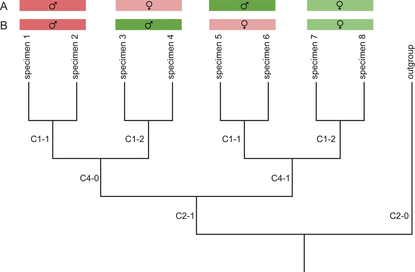
Figure 1 Potential influence of directed noise on tree topology. Directed noise because of sexual dimorphism, for example, can lead to misleading topologies. In this hypothetical tree, colours indicate the ‘true' species (which we usually do not know in palaeontological datasets), tones and symbols the sexes. (A) The result when character 1 codes for a sexually dimorphic trait that equally occurs in both species. (B) The result if character 4 coded a sexually dimorphic feature. In case (B), character 1 codes for the true distinguishing feature between the species, but is overprinted by character 4, which codes for features shared among males or females across the two species. Mapping the character states diagnosing the subclades might help detect these phenomena: if distantly related subclades show the same diagnostic features (the different states of character 1 in the present example), they should be checked for potentially being sexually dimorphic.
Ecological or functional convergences can occur differently in subsets of characters, resulting in an uneven distribution of homoplasy among the available characters. Such an uneven distribution has been shown to occur in mammals, where dental characters are more homoplastic than other osteological ones, and produce trees that are less compatible with molecular trees than the ones recovered using only non-dental osteological characters (Sansom et al. Reference Sansom, Wills and Williams2017). Such a different phylogenetic signal might indicate that teeth carry a largely functional signal instead of a phylogenetic one, and that, in extreme cases, the phylogenetic signal is overprinted by a functional and/or ecological signal. In order to assess if a dataset is affected by such an overprinting, it might be advisable to check if different subsets of characters carry different signals. This can be done by using Partitioned Bremer Support (see Parker Reference Parker2016), or by dissecting the dataset into smaller sets including only the group of characters in question (e.g., dental versus cranial versus postcranial), and comparing the outcomes with a series of tests, as described in detail by Sansom et al. (Reference Sansom, Wills and Williams2017).
Whereas the exclusion of homoplastic characters appears counter-productive, and negative effects can best be avoided by adding OTUs, this does not mean that highly homoplastic characters should have the same weight as highly parsimony-informative ones (Farris Reference Farris, Platnick and Funk1983; Goloboff Reference Goloboff1993, 1995; Chippendale & Wiens 1994). This has led several workers (e.g., Farris Reference Farris1969; Goloboff et al. Reference Goloboff, Farris and Nixon2008a, Goloboff Reference Goloboff2014) to propose methods for identifying and downweighting homoplasies (see Section 1.2.1 for discussion of the different strategies), but these have not previously been considered in detail with respect to their utility in specimen-level phylogenetic analyses. In short, the most justified approach in character selection would be to use as many character statements as possible, including highly variable ones, as long as the latter do not include a high percentage of missing data.
1.1.3. Missing data
Missing entries can stem from both incompletely preserved specimens (particularly in vertebrate palaeontology, and in analyses at specimen level) and incompletely scored characters (Kearney & Clark Reference Kearney and Clark2003; Pol & Escapa Reference Pol and Escapa2009; Mannion & Upchurch Reference Mannion and Upchurch2010; Tschopp et al. Reference Tschopp, Tschopp and Mateus2018b). There is an expectation that, all things being equal, missing data are a particular problem for specimen-level analyses because greater completeness of OTUs in a conventional analysis is often achieved by combining multiple specimens into a single OTU. Whereas the use of individual specimens as OTUs reduces the risk of having chimeric higher-level OTUs, it will also tend to increase the relative amount of missing data per OTU. This would especially be the case when palaeontological species-level datasets are simply converted into specimen-level matrices. However, the challenge is not necessarily the missing data per se, but the amount of anatomical overlap between the included OTUs (see Section 1.1.1). Also, the relative amount of missing data in a palaeontological specimen-level analysis is not always higher when compared to species-level matrices (Table 2). It is, therefore, important to consider the real contents of a species-level OTU – if it only comprises an individual specimen, this should be stated clearly in the matrix. In fact, given that many fossil vertebrate species are only represented by a single specimen, phylogenetic analyses, even when formally run at species-level, are effectively often partial specimen-level analyses. Exceptions are analyses using similar matrices at different taxonomic levels, as, for instance, was done by Tschopp & Mateus (Reference Tschopp and Mateus2017), who used a species-level matrix based on the specimen-level matrix of Tschopp et al. (Reference Tschopp, Mateus and Benson2015). In their case, the amount of missing data was considerably reduced from 65 % (complete taxon sampling) or 70 % (only ingroup) in the specimen-level matrix to 49 % (complete) and 53 % (ingroup) in the species-level matrix (Table 2).
This reduction can also be quantified using the Character Completeness Metrics proposed by Mannion & Upchurch (Reference Mannion and Upchurch2010), which considers the percentage of phylogenetic characters that can be scored for a specimen or species. The Chinese sauropod Euhelopus zdanskyi, for instance, is known from two incomplete specimens (Wiman Reference Wiman1929; Wilson & Upchurch Reference Wilson and Upchurch2009). The more complete one (PMU 24705) scores 47 % in character completeness, whereas, at the level of species, combining information from both specimens, character completeness increases to 68 % (Mannion & Upchurch Reference Mannion and Upchurch2010).
The metrics of Mannion & Upchurch (Reference Mannion and Upchurch2010) are particularly low in sauropodomorph type specimens, which, on average, are only slightly more than half as complete as the species they typify, reaching 25.65 % of individual skeletal completeness. The situation is considerably better in ichthyosaurs, where holotype specimens have an average skeletal completeness of 45.49 % (ranging from 1 to 90.5 %), and reach 66 % of the completeness of the entire species (Table 3; based on data from Cleary et al. Reference Cleary, Moon, Dunhill and Benton2015). Whereas the completeness of sauropodomorph type specimens increased through time of description (Mannion & Upchurch Reference Mannion and Upchurch2010), there seems to be no such correlation in ichthyosaurs (Fig. 2). In any case, because species-level OTUs can always draw on one or more specimens, they are logically always equally or more complete than a specimen-level OTU.
Table 3 Skeletal completeness of holotype specimens of ichthyosaurs, and the species they typify. Data from Cleary et al. (Reference Cleary, Moon, Dunhill and Benton2015).

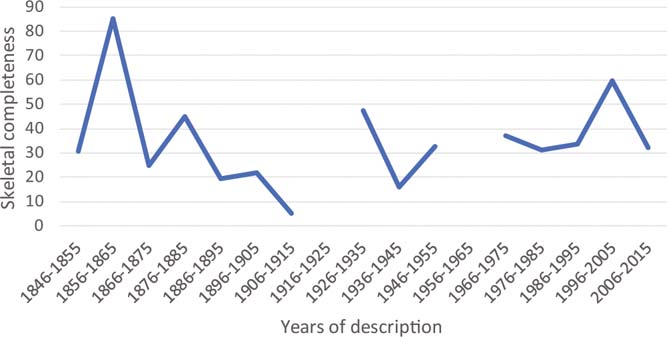
Figure 2 Skeletal completeness of holotype specimens of ichthyosaurs. Average completeness of species erected within ten-year bins from 1846 to 2015 are plotted. No species was erected between 1916 and 1925, and 1956 and 1965. Data from Cleary et al. (Reference Cleary, Moon, Dunhill and Benton2015).
The inclusion of highly incomplete specimens results in an extensive lack of anatomical overlap among the specimen-level OTUs in the matrix, and is likely to decrease resolution in the consensus trees (Huelsenbeck Reference Huelsenbeck1991; Kearney & Clark Reference Kearney and Clark2003; Wiens Reference Wiens2006; Butler & Upchurch Reference Butler and Upchurch2007; Prevosti & Reference Prevosti and ChemisquyChemisquy 2010; Tschopp et al. Reference Tschopp, Mateus and Benson2015, Reference Tschopp, Tschopp and Mateus2018b). Both simulations and real case studies have shown that an increase in the relative amount of missing data lowers accuracy and increases errors (Wiens Reference Wiens2006; Prevosti & Chemisquy Reference Prevosti and Chemisquy2010; Sansom Reference Sansom2015). However, these case studies deleted information from already existing matrices, so that the result is not really about the impact of missing data in general, but about not including available data a priori, and thus the negative impact might be expected. When adding taxa or characters, even if they include a substantial amount of missing entries, accuracy increases in most cases, or at least remains similar to that achieved by the original matrix (Wiens Reference Wiens2006). Because missing data is no data, it cannot logically be added when adding incompletely scored characters or taxa – what we add is the amount of actual data scored in them. Therefore, even if the addition of more taxa and/or characters results in a relative increase of missing data in the entire dataset, we still increase the absolute amount of data that can be analysed, so that the positive results obtained by Wiens (Reference Wiens2006) are to be expected.
Another concern is that character statements with a large number of missing entries may simulate the problem of long-branch attraction (Wiens Reference Wiens2006). This problem arises from the presence of two OTUs or characters, for which few data are available, but the information that is available might be convergent, as can be the case in highly homoplastic characters (see Section 1.1.2). Without the information on the true character-state distribution across the tree (because of too many missing entries), the two convergent taxa might be wrongly grouped together to the exclusion of others (Bergsten Reference Bergsten2005; Wiens Reference Wiens2006; Tschopp et al. Reference Tschopp, Tschopp and Mateus2018b). However, even though adding new OTUs or characters might decrease the overall anatomical overlap in the dataset (Tschopp et al. Reference Tschopp, Tschopp and Mateus2018b), the addition of data is always recommended (Kearney & Clark Reference Kearney and Clark2003; Wiens Reference Wiens2006; Goloboff Reference Goloboff2014). The relative amount of missing data should, thus, not be reduced by omitting taxa or characters; rather, its deleterious effects should be addressed using approaches such as differential weighting and ‘reduced consensus', as will be discussed in Sections 1.2.1 and 1.2.3. Moreover, one way in which choice of character construction can reduce missing data is to convert multistate characters (coded within a single column in the data matrix) into their equivalent additive binary form. Although this is only appropriate for those multistate characters that capture a morphological transition series (i.e., ordered; see Section 1.2.2), the use of additive binary coding has the benefit of reducing the amount of missing data. For example, a single multistate character scoring the number of vertebrae in the neck would have to be scored as ‘?' whenever the neck of a specimen was incompletely preserved, but can be scored for at least some of the states for the equivalent additive binary character (e.g., a combination of 0s, 1s and ?s scores would inform the analysis that the specimen had at least a given number of neck vertebrae, even though the exact number remains unknown – see Upchurch (Reference Upchurch1998) for elaboration of this point).
1.1.4. Character-state scoring
Characters can be coded either in a discrete way or as continuous characters. These continuous characters are a type of quantitative character that use the specific ratios, ranges of measurements or specific numbers in meristic features as states (Goloboff et al. Reference Goloboff, Mattoni and Quinteros2006). As such, this approach further develops the idea of gap-weighting (Thiele Reference Thiele1993), in which large differences in quantitative traits between OTUs are upweighted compared to minute ones, but avoids discretisation of the actual values obtained from the OTUs (Goloboff et al. Reference Goloboff, Mattoni and Quinteros2006). Advocates of such an approach mostly highlight the fact that state boundaries in discrete, quantitative character statements are often arbitrary, and their choice rarely explained and justified by the researchers (see Rae Reference Rae1998, and references therein). Thus, the risk of influencing the analysis by choosing state boundaries that favour the recognition of a pre-conceived clade is relatively high (Mannion et al. Reference Mannion, Upchurch, Barnes and Mateus2013).
The implementation of continuous characters in the phylogenetics software TNT treats them by default as ordered (Goloboff et al. Reference Goloboff, Mattoni and Quinteros2006). Thus, given that every single score forms its own character state, the sum of steps in a single continuous character is much higher than any discrete binary character. As already pointed out by Goloboff et al. (Reference Goloboff, Mattoni and Quinteros2006), there are weighting strategies that can be applied to address this issue, which will be discussed in Section 1.2.1.
General issues with this approach concern the choice of exact values or ranges as character scores, the use of mean or maximum or minimum values, and how to address incompleteness and deformation in fossils. Although these issues apply to any kind of phylogenetic analysis, they are particularly common when working at the specimen level, mostly because the sample size on which ratios and other values can be based is much lower than when working with species or higher-level taxa (e.g., some ranges, means, etc. will be based on a maximum sample size of two, like, for instance, the tibia:femur ratio in a single individual, or cannot be obtained from individual specimens, because of incompleteness).
Rae (Reference Rae1998) argued for the use of means or medians in the scoring of continuous characters, because variation could occur randomly or due to measurement errors, rendering ‘central tendencies' (as he termed them) more appropriate estimations of the actual distribution of values within an OTU. When working with fossils, taphonomic deformation can add to the variation of numerical values, and even lead to differential character scoring (Tschopp et al. Reference Tschopp, Russo and Dzemski2013), in particular when using continuous data. As exemplified in Figure 3, two cervical vertebrae of a single sauropod individual (SMA 0011, the holotype of Galeamopus pabsti, in this case) can be compressed transversely (Fig. 3a) or dorsoventrally (Fig. 3b), which leads to highly diverging shapes and ratios. Furthermore, specimen incompleteness might skew the analysis towards an extreme when only a statistical outlier can be sampled. If only a single, incomplete element is preserved from a specimen, it could even be that the incompleteness renders it impossible to obtain precise measurements and ratios (and thus precludes scoring as continuous characters), although they might be scorable in a discrete version of the character (Mannion et al. Reference Mannion, Upchurch, Barnes and Mateus2013). For instance, no exact ratios concerning tibial robustness are obtainable from a tibia lacking its distal end, but the preserved length might still result in a robustness ratio that exceeds the defined boundary of a discretised state (e.g., the proximal-width-to-proximodistal-length ratio might be ‘0.15 or lower', showing that it lies below the state boundary of 0.2). In this case, a continuous character could not be scored when using central tendencies, but one could argue that a range could be included. This range could span from the ratio using the preserved length as minimum value to the highest value exhibited by any other OTU. However, such a range would exaggerate the actual variability and overlap with a large number of more precise ranges from other individuals, effectively hiding phylogenetic information (Giovanardi Reference Giovanardi2017). Taphonomically increased ranges due to deformation processes pose the same problem.

Figure 3 Taphonomic deformation impacts measurements and ratios. The cervical vertebrae 5 (A) and 8 (B) of Galeamopus pabsti SMA 0011 were compressed transversely and dorsoventrally, respectively. Anterior condyle outline shape and ratios such as centrum height/width across parapophyses are examples of affected measurements and ratios potentially useful for phylogenetic analysis. Minimum and maximum values or ranges can, therefore, yield misleading data for continuous character scores, and central tendencies such as means should be preferred. Abbreviations: cH = centrum height; h = height; nc = neural canal; pap = parapophysis; paW = width across parapophyses; prz = prezygapophyses; tp = transverse process; w = width. Vertebrae figured in anterior view (modified from Tschopp & Mateus Reference Tschopp, Tschopp and Mateus2017), and scaled to the same anterior condyle height.
Given that it is statistically more probable that a single element found from a vertebral column, for instance, is closer to the central tendency than to any minimum or maximum value displayed along the column, and given that ranges pose their own risks, especially when working with fossils, mean or median values should be preferred over ranges, or minimum or maximum values. Discretisation of a quantitative character can be useful in ratios that are more prone to deformational processes (Arbour & Currie Reference Arbour and Currie2012; Tschopp et al. Reference Tschopp, Russo and Dzemski2013), effectively hiding potentially misleading information. However, state boundaries in discrete characters should be defined based on statistical analyses rather than on preconceived taxonomic or phylogenetic interpretations. There is a large number of papers concerning discretisation of continuous data in statistics (e.g., Jiang & Sui Reference Jiang and Sui2015; Cano et al. Reference Cano, Nguyen, Ventura and Cios2016, and references therein), and some methods are also implemented in the usual office packages for computers. To our knowledge, a study on which kind of discretisation would work best in phylogenetics has not yet been made.
1.1.5. Polymorphisms
Polymorphic traits are traits that are variable within species (Wiens Reference Wiens1995, Reference Wiens and Wiens2000). At the species level, they can be treated differently, and several theoretical approaches have been compared by Wiens (Reference Wiens1995, Reference Wiens and Wiens2000), who suggested the use of a frequency approach, meaning that species should be scored for the character state that occurs with the highest frequency within the species. By splitting a species-level OTU into single specimens, some polymorphisms can be avoided, because they derive from intraspecific variability.
Although reducing polymorphisms deriving from intraspecific variability, a specimen-level approach can still be affected by polymorphisms. In single specimens, these can be created by serial variation throughout the vertebral column (e.g., Barbadillo & Sanz Reference Barbadillo and Sanz1983; Wilson Reference Wilson2012; Chamero et al. Reference Chamero, Buscalioni, Marugán-Lobón and Sarris2014; Böhmer et al. Reference Böhmer, Rauhut and Wörheide2015; Tschopp Reference Tschopp, Wings, Frauenfelder and Rothschild2016), bilateral asymmetry (e.g., Palmer Reference Palmer1996; Hoso et al. Reference Hoso, Asami and Hori2007) or pathologic processes (e.g., Rothschild & Martin Reference Rothschild and Martin2006; Foth et al. Reference Foth, Evers, Pabst, Mateus, Flisch, Patthey and Rauhut2015; Tschopp et al. Reference Tschopp, Wings, Frauenfelder and Rothschild2016). Whereas an exclusion of pathologic data is advisable for obvious reasons, serial variation and bilateral asymmetry can still provide important phylogenetic data (Palmer et al. Reference Palmer, Strobeck, Chippindale and Markow1994; Böhmer et al. Reference Böhmer, Rauhut and Wörheide2015). Even though polymorphisms in a single specimen-level OTU might indicate that the trait is individually variable and has no phylogenetic/taxonomic significance, this is difficult to establish a priori and should be evaluated in light of specimen-level relationships – exclusion is, therefore, not an appropriate option (Wiens Reference Wiens1998; Poe & Wiens Reference Poe, Wiens and Wiens2000). In serially variable traits, frequency-based approaches could work in a similar way as in the studies reported by Wiens (Reference Wiens1995, Reference Wiens and Wiens2000). In vertebral columns with distinct regionalisation (see Müller et al. Reference Müller, Scheyer, Head, Barrett, Werneburg, Ericson, Pol and Sánchez-Villagra2010 for a review in tetrapods), it can also make sense to subdivide the column into separate morphological areas, as is often done in sauropod dinosaurs and squamates (see, e.g., the descriptions and characters for anterior cervical, or posterior caudal vertebrae in Carballido et al. Reference Carballido, Salgado, Pol, Canudo and Garrido2012; D'Emic Reference D'Emic2012; Gauthier et al. Reference Gauthier, Kearney, Maisano, Rieppel and Behlke2012; Mannion et al. Reference Mannion, Upchurch, Barnes and Mateus2013; Otero et al. Reference Otero, Soto-Acuña, O'Keefe, O'Gorman, Stinnesbeck, Suárez, Rubilar-Rogers, Salazar and Quinzio-Sinn2014; Tschopp et al. Reference Tschopp, Mateus and Benson2015, Reference Tschopp, Villa, Camaiti, Ferro, Tuveri, Rook, Arca and Delfino2018c). Often, such subdivisions are made numerically, because clear-cut morphological boundaries are difficult to identify (Mannion et al. Reference Mannion, Upchurch, Barnes and Mateus2013; Tschopp et al. Reference Tschopp, Mateus and Benson2015), but increasing information is now available on serial variation in a number of vertebrate animals based on geometric morphometrics, so that more detailed and less arbitrary morphological subdivisions can be made (e.g., Müller et al. Reference Müller, Scheyer, Head, Barrett, Werneburg, Ericson, Pol and Sánchez-Villagra2010; Burnell et al. Reference Burnell, Collins and Young2012; Böhmer et al. Reference Böhmer, Rauhut and Wörheide2015). Splitting vertebral columns into subregions is an analogous approach to subdividing taxa into lower-level taxonomic units in order to minimise the number of polymorphisms. A combination of character splitting and frequency-based scoring approaches, therefore, seems the best option in this case, even though this would also increase the relative amount of missing data.
Bilaterally asymmetric traits can occur due to developmental plasticity or as a result of abnormal developmental processes. Whereas the latter should be treated as pathology and excluded, the first could still be phylogenetically informative because it may indicate a trend to acquiring a new feature that may become fixed by natural selection (Palmer Reference Palmer1996). Distinguishing between the two may be difficult in fossils, but in systems where asymmetry is ubiquitous, as, for instance, in the lamination pattern of vertebrae of saurischian dinosaurs (Wilson Reference Wilson1999, Reference Wilson2012), it is probably safe to assume they derive from plasticity instead of widespread pathology.
Generally, only a small number (usually two) of bilaterally occurring elements are present in a vertebrate skeleton. Frequency-based, or majority approaches, therefore, cannot be applied. Possible treatments of such characters outlined by Wiens (Reference Wiens1995) include: (1) the ‘any-instance' method, where the sheer occurrence of a trait (even if only on one of several equivalent elements) is treated as if the character state was invariably present; (2) the ‘missing' method, where asymmetric traits are scored as missing data; (3) the ‘polymorphic' method includes polymorphic scores; (4) the ‘scaled', ‘unordered' or ‘unscaled' methods, where binary characters are coded such that they include a third polymorphic character state as state 1. The character can then be treated as ordered (‘scaled') or unordered, and binary characters, where no asymmetry was observed can be coded as normal binary character statements, without a polymorphic intermediate state (‘unscaled', see Wiens Reference Wiens1995 for more details). The ‘any-instance' method would be the most straight forward approach in a specimen-level analysis, but ignores a potential phylogenetic signal in the occurring asymmetry. Also, it remains unclear how to score an asymmetrical individual in a multistate character, following this method (Wiens Reference Wiens1995). Scoring a specimen as ‘?' in the trait in which it shows bilateral asymmetry results in loss of information, and the same happens when using the polymorphic approach if the character is binary, because the analysis treats a polymorphic score in binary character statements as ‘?' (Wiens Reference Wiens1995, Reference Wiens1998; Brazeau Reference Brazeau2011). Of the two latter treatments, a score as polymorphic at least provides information to a researcher who inspects the data matrix, because it clearly indicates the presence of two or more states, whereas a score as ‘missing' completely hides any information. The treatments that include the most potential phylogenetic information are those where a separate polymorphic character state is included (in the present case, this state might be called ‘bilaterally asymmetric'). When applying this approach to a real dataset, the scaled method yielded the highest accuracy, although without large differences compared to the unscaled method (Wiens Reference Wiens1998).
Bilateral asymmetries can be an issue in continuous characters, in particular in meristic features. For instance, tooth counts in lizard dentaries and maxillae often vary in left and right elements (Arnold et al. Reference Arnold, Arribas and Carranza2007). Given that these variations are usually small, and counts generally precise, this might be a case where scoring ranges could actually be helpful in order to include as much morphological information as possible, without risking widely overlapping ranges among large numbers of individuals in the dataset.
1.1.6. Ontogenetic traits
As previously mentioned, ontogenetically variable traits can introduce problems into specimen-level analyses. However, there are several approaches one can adopt during scoring and subsequent steps in the analysis, if it is necessary to include a juvenile specimen. In sauropod dinosaurs, the number and prominence of vertebral laminae, and vertebral pneumatisation, strongly increases during ontogeny (Wilson Reference Wilson1999; Wedel et al. Reference Wedel, Cifelli and Sanders2000; Wedel Reference Wedel2003; Bonnan Reference Bonnan2007; Schwarz et al. Reference Schwarz, Ikejiri, Breithaupt, Sander and Klein2007; Tschopp & Mateus Reference Tschopp, Tschopp and Mateus2017), which led Carballido & Sander (Reference Carballido and Sander2014) to propose four Morphological Ontogenetic Stages (MOS) applicable to sauropod vertebrae. In the case of Europasaurus holgeri, Carballido & Sander (Reference Carballido and Sander2014) found that when scoring all the different MOS as distinct OTUs in the phylogenetic analysis, the juvenile MOS 1 and 2 occurred in a more ‘basal' position compared to MOS 3 and 4. This is probably due to the fact that a large number of vertebral character statements used in sauropod dinosaur phylogenetics code for variation in these traits, and that well-developed lamination and pneumatisation is both an adult and a phylogenetically derived feature among sauropods (Wilson Reference Wilson2012). Many other ontogenetically variable features are known in the vertebrate skeleton, so that the most straightforward approach would simply be to avoid scores of ontogenetically variable traits in obviously juvenile specimens. If scored, these characters can be downweighted during the analysis, and not considered for species delimitation (see Sections 1.2.1 and 1.3.1), but the exclusion of these scores altogether would probably still be more methodologically sound.
1.2. Phylogenetic methodology
1.2.1. Character weighting
Specimen-level analyses provide an opportunity to include characters coding for minute differences in morphology, and check whether or not they might be informative at some taxonomic level. However, such characters might not have a genetic basis, but could represent individual variation caused by plasticity, ecophenotypic effects or any other non-genetic cause (Tschopp et al. Reference Tschopp, Mateus and Benson2015), which manifests as homoplasy in the phylogenetic analysis (see Section 1.1.2). In such cases, equal weighting is not advisable, in particular when working with large-scale specimen-level analyses. Indeed, Goloboff et al. (Reference Goloboff, Farris and Nixon2008a, Reference Goloboff, Torres and Arias2018) have shown that weighting against homoplasy increased the reliability and stability of tree topologies in morphological datasets.
Downweighting can be implemented a priori, or during the tree search, or iteratively after each tree search (Farris Reference Farris1969; Goloboff Reference Goloboff1993, Reference Goloboff2014; De Laet Reference De Laet1997; Goloboff et al. Reference Goloboff, Farris and Nixon2008a). The most intuitively correct, and least subjective way, to downweight potential homoplasies is to use a method called ‘implied weighting' (Goloboff Reference Goloboff1993), which is implemented in the phylogenetic software package TNT (Goloboff et al. Reference Goloboff, Carpenter, Arias and Esquivel2008b). This approach downweights characters with widespread homoplasy as part of the tree search function (Goloboff Reference Goloboff1993, Reference Goloboff2014; Goloboff et al. Reference Goloboff, Farris and Nixon2008a, Reference Goloboff, Torres and Arias2018). The equation is as follows:
 $${ weight} = k / (k + [ { observed\ steps - minimum\ steps} ] )$$
where k is the ‘concavity value'.
This equation shows that implied weighting can be performed with different concavity values (‘k-values'; Goloboff Reference Goloboff1993, Reference Goloboff1995, Reference Goloboff2014). These values describe the slope of the curve, defining how strongly characters with different homoplastic rates are downweighted. The lower the k-value, the more strongly a highly homoplastic character is downweighted during the phylogenetic analysis compared to a less variable character. A k-value approaching zero would, therefore, effectively exclude homoplastic characters, whereas one approaching infinity would weight them all equally. However, other than avoiding extreme values, there seems to be little biological or methodological basis for selecting any specific k-value (Goloboff Reference Goloboff1995; Turner & Zandee Reference Turner and Zandee1995). Recent studies showed that a k-value of around 12 produced the most accurate results in a series of morphological datasets (Goloboff et al. Reference Goloboff, Torres and Arias2018), but it is possible that this value varies slightly in different taxa, or even in different phylogenetic analyses of a single taxon. However, this cannot be used as an argument to dismiss implied weighting a priori, it just means that one should perform different analyses with varying k-values, and compare the results (Goloboff et al. Reference Goloboff, Farris and Nixon2008a) by using statistical or stratigraphic measurements, as will be discussed in Section 1.2.3. Ultimately, implied weighting might provide a simple solution to the problem found by Sites et al. (Reference Sites, Davis, Guerra, Iverson and Snell1996): that is, the exclusion of all homoplastic characters reduced accuracy, whereas the exclusion of only the most homoplastic ones increased it.
Implied weighting as initially proposed by Goloboff (Reference Goloboff1993) can be negatively influenced by missing data, because characters with a large amount of the latter have a higher probability of showing fewer homoplasies, and would thus tend to be upweighted relative to more completely scored characters (Goloboff Reference Goloboff2014). In a worst-case scenario, where the data set includes very incompletely scored characters, the weaker downweighting could effectively lead to a strengthening of the long-branch attraction phenomenon simulated by the missing data (Wiens Reference Wiens2006; Tschopp et al. Reference Tschopp, Tschopp and Mateus2018b). Nonetheless, real case studies using matrices with missing data showed that implied weighting approaches performed better than equal weighting (Prevosti & Chemisquy Reference Prevosti and Chemisquy2010). Moreover, Goloboff (Reference Goloboff2014) implemented the so-called ‘extended implied weighting' approach in the software TNT, which not only downweights the characters based on their homoplastic rate and the chosen k-value, but also adapts the k-value for every character individually based on its proportion of missing entries. Congreve & Lamsdell (Reference Congreve and Lamsdell2016) dismissed this methodology, in part, because polymorphic or inapplicable characters are often treated as missing data and could, therefore, be wrongly penalised by an extended implied weighting approach. However, the proposed methodology actually just enables the use of different k-values for every single character (Goloboff Reference Goloboff2014), so that these issues could also be addressed manually instead of applying the default, automated script (Goloboff et al. Reference Goloboff, Torres and Arias2018). Moreover, at least inapplicable character states can be recognised by the latest versions of TNT and, thus, be excluded from the algorithms for extended implied weighting (Goloboff et al. Reference Goloboff, Torres and Arias2018).
Simulations using modelled phylogenies have recently shown that traditional implied weighting performs worse than equal weighting and probability-based approaches such as Bayesian (Congreve & Lamsdell Reference Congreve and Lamsdell2016; O'Reilly et al. Reference O'Reilly, Puttick, Parry, Tanner, Tarver, Fleming, Pisani and Donoghue2016). On the other hand, case studies using real morphological matrices appear to show the contrary (Prevosti & Chemisquy Reference Prevosti and Chemisquy2010; Brinkman et al. Reference Brinkman, Rabi and Zhao2017), and also extended implied weighting seemed to work well under certain circumstances when analysing specimen-level data in lizards (Villa et al. Reference Villa, Tschopp, Georgalis and Delfino2017). One reason for these discrepant conclusions could be that the modelled phylogenies did not accurately represent a real distribution of homoplasy within a morphological dataset (Goloboff et al. Reference Goloboff, Torres and Arias2018). By analysing the actual distribution of homoplasies in numerous morphological data sets, Goloboff et al. (Reference Goloboff, Torres and Arias2018) showed that earlier simulations (Congreve & Lamsdell Reference Congreve and Lamsdell2016; O'Reilly et al. Reference O'Reilly, Puttick, Parry, Tanner, Tarver, Fleming, Pisani and Donoghue2016) did, indeed, represent this distribution incorrectly. Comparisons of the methodologies with newly simulated trees based on the distribution of homoplasies found in real data sets resulted in extended implied weighting being the strategy that recovered the most accurate trees, followed by the traditional implied weighting approach (Goloboff et al. Reference Goloboff, Torres and Arias2018). Even though implied weighting retrieved a proportionally larger number of both correct and incorrect groupings in data sets with more homoplasy, compared to equal weights (Congreve & Lamsdell Reference Congreve and Lamsdell2016; Goloboff et al. Reference Goloboff, Torres and Arias2018), the relative amount of added correct groups exceeded the relative increase of incorrect groups, thereby increasing overall accuracy, especially when using extended implied weighting (Goloboff et al. Reference Goloboff, Torres and Arias2018). Collapsing branches with low support was shown by Goloboff et al. (Reference Goloboff, Torres and Arias2018) to reduce the number of incorrect groups, but this also reduces the number of weakly supported, correct groups (Goloboff et al. Reference Goloboff, Torres and Arias2018), and generally lowers the information content of the recovered trees by increasing the number of polytomies.
These issues become especially important if the matrix was specifically constructed to test assumptions of homology at the level of single individuals, which likely results in more homoplasies in the data set. At present, it is not yet clear whether a stronger downweighting function might help to reduce the number of incorrect retrieved groups in data sets with a larger amount of homoplasies, and if these incorrect groups might be identified somehow if we do not know the correct tree. Moreover, only Goloboff et al. (Reference Goloboff, Torres and Arias2018) also included the extended implied weighting approach in their simulations, and most other studies used rather strong downweighting functions (e.g., k=1, 3, 5 and 10 in Congreve & Lamsdell Reference Congreve and Lamsdell2016). Additional tests with real data sets (such as that of Villa et al. Reference Villa, Tschopp, Georgalis and Delfino2017) and a higher range of downweighting functions will be needed to compare the performance of different weighting methods, including extended implied weighting, in order to resolve this debate.
Tschopp et al. (Reference Tschopp, Mateus and Benson2015) noted that using an implied weighting strategy was useful to address the potentially misleading ontogenetically variable characters, because the ontogenetic changes add variability to these characters, which, therefore, have a higher homoplastic rate, and so are downweighted more strongly than less variable ones. However, if the characters are highly parsimony-informative among adult specimens, the variability introduced by juvenile specimens would partly obscure this information, and, combined with implied weighting, even reduce its impact on the calculation of the most-parsimonious trees. Omitting scores for ontogenetically variable traits in obviously juvenile specimens, therefore, appears more appropriate than applying implied weighting to reduce their deleterious effects.
1.2.2. Character ordering
Phylogenetic characters can have multiple states that describe different relative sizes or shapes of a single feature. Multistate characters can be treated as ordered or unordered, or with step-matrices (Hauser & Presch Reference Hauser and Presch1991; Wilkinson Reference Wilkinson1992; Wilson Reference Wilson2002; Brazeau Reference Brazeau2011). Ordering and step matrices impose different degrees of directional morphological state transformations onto the character concerned, whereas a treatment as unordered accepts all possible changes between character states as equally probable (Wilkinson Reference Wilkinson1992; Brazeau Reference Brazeau2011). For instance, in an ordered character with three states (0, 1, 2), a morphological change from state 0 to state 2 would need two evolutionary steps, and thus also increase the length of the most-parsimonious tree relative to a treatment of the same character as unordered. By using a step-matrix, a researcher can define the possible direct evolutionary steps even more precisely, and can allow for a so-called ‘easy loss character', in which the evolution from character state 0 to 2 costs more than from 2 to 0, implying that it is more likely that the character will pass through state 1 on its evolutionary way to 2, whereas the reversal could be direct (Wilson Reference Wilson2002). The differences and rationales of why, how and if multistate characters should be ordered have been reviewed recently by Brazeau (Reference Brazeau2011), and apply to phylogenetic analyses at any taxonomic level equally, so that there is no need to discuss it in detail here. Brazeau (Reference Brazeau2011) concluded that multistate characters should be ordered if they code for quantitative characters, or if they describe an obvious morphological transformational series. We follow this recommendation here. The use of step-matrices, even if theoretically adding methodological soundness, probably has little influence on the result in most cases, but needs additional time investment to prepare the file for the analysis. The implementation of which characters should be ordered, on the other hand, is uncomplicated and fast.
1.2.3. Tree searches and consensus trees
Whereas no specific requirements apply to the methodology of tree searches when using specimen-level matrices, several points have to be addressed once a set of trees has been obtained, and before proceeding to species delimitation. The basic tree topology can be influenced by ontogenetically variable characters, consensus methods can hide phylogenetic structure and analyses under differential weighting (as recommended in Section 1.2.1) can produce conflicting tree topologies.
Ontogenetically variable characters can influence tree topology, and thus also taxonomic interpretations. If one prefers downweighting over exclusion of ontogenetic character states (as in Tschopp et al. Reference Tschopp, Mateus and Benson2015), the position of juvenile specimens in the phylogenetic trees, on which species delimitation will be based, will be influenced by these characters. Another approach was followed by Campbell et al. (Reference Campbell, Ryan, Holmes and Schröder-Adams2016), who conducted a specific test to assess the influence of ontogeny on tree topology. They followed the principles of a ‘ontogenetic analysis' as initially proposed by Brochu (Reference Brochu1996), and ran it in parallel to the phylogenetic analysis. In an ontogenetic analysis, only traits known to be ontogenetically variable are used as character statements (Brochu Reference Brochu1996; Carr & Williamson Reference Carr and Williamson2004; Campbell et al. Reference Campbell, Ryan, Holmes and Schröder-Adams2016). Character states are adapted to follow supposed ontogenetic changes, and multistate characters are treated as ordered during the parsimony analysis.
Campbell et al. (Reference Campbell, Ryan, Holmes and Schröder-Adams2016) used their ontogenetic analysis to check if small-to-large-sized skulls of two different species of Chasmosaurus fell on two distinct ontogenetic trajectories, which could be used to distinguish the two species. Although the result of their study was negative, such an approach could also be used to verify if the topology of the tree recovered by the ontogenetic analysis reproduces the findings of the phylogenetic one. If this is the case, and if the ontogenetic trajectory also correlates with an increase in body size, one should expect that the topology found by both analyses was strongly influenced by ontogenetically variable characters. Such an integrative approach of ontogenetic and phylogenetic analysis is probably more appropriate than simply reducing the weight and, thus, impact of ontogenetic character states as done by Tschopp et al. (Reference Tschopp, Mateus and Benson2015). A combination of an ontogenetic analysis and the exclusion of obviously juvenile character states during scoring for the phylogenetic analysis under implied weighting approaches would likely provide the most accurate results.
Most specimen-level analyses of fossil taxa have had to cope with the problem of a very high number of most-parsimonious trees, and, therefore, large polytomies in the strict consensus tree (Yates Reference Yates2003; Scannella et al. Reference Scannella, Fowler, Goodwin and Horner2014; Tschopp et al. Reference Tschopp, Mateus and Benson2015; Campbell et al. Reference Campbell, Ryan, Holmes and Schröder-Adams2016). Polytomies can derive from both the genuine absence of a branching pattern (so-called ‘hard polytomies'), and insufficient data in the phylogenetic matrix to recover an entirely resolved tree (‘soft polytomies'; Maddison Reference Maddison1989; Purvis & Garland Reference Purvis and Garland1993). Thus, in the context of specimen-level analyses, hard polytomies would represent the lack of phylogenetic structure below the level of species, and could be used as an indication for the delimitation of species (see Section 1.3.1 for a detailed assessment). However, complete strict consensus trees do not always report the entirety of phylogenetic signal present in the matrix (Wilkinson Reference Wilkinson1995), so a distinction of hard and soft polytomies is crucial before making positive inferences based on an apparent lack of hierarchical structure. It is possible that a few, highly unstable, taxa (specimens in this case) might produce large soft polytomies, even though the rest of the included OTUs remain stable (Wilkinson Reference Wilkinson1995). Often, the main reason for this instability is missing data in fragmentary specimens lacking anatomical overlap (see Section 1.1.3). One approach to ameliorate such a problem is to prune the unstable OTUs from the trees a posteriori, and then apply tests to identify their most-parsimonious phylogenetic positions (e.g., see Tschopp et al. Reference Tschopp, Mateus and Benson2015). The underlying tree structure hidden in ‘soft polytomies' in the complete strict consensus tree can, thus, be revealed by reduced strict consensus approaches, or a posteriori pruning of the most unstable taxa.
Multiple conflicting tree topologies can be generated by the presence of unstable taxa, as discussed previously, but can also occur because of the application of an array of different starting assumptions or analytical protocols to the same data set. Thus, alternative positions of specimens have to be tested with a number of approaches. There are several support measures to evaluate tree accuracy. Given that these are not specific to specimen-level phylogeny, we will only discuss them briefly herein. Following our recommendation to use different weighting strategies during phylogenetic analysis, we will specifically focus on the impact of weighting on the various support measures.
The most widely used support metrics are resampling measures such as bootstrapping and jackknifing. Källersjö et al. (Reference Källersjö, Albert and Farris1999) and Goloboff et al. (Reference Goloboff, Farris and Nixon2008a) used jackknife frequencies to calculate and compare group support between analyses with different character sets or weighting strategies. Källersjö et al. (Reference Källersjö, Albert and Farris1999) compared analyses based on molecular data under equal weighting, with and without the highly homoplastic third-codon positions, whereas Goloboff et al. (Reference Goloboff, Farris and Nixon2008a) compared different k-values in implied weighting. The two approaches are equivalent, because equal weighting and the exclusion of characters basically represent the two extremes of k-values in implied weighting (Goloboff Reference Goloboff1993; De Laet Reference De Laet1997). However, jackknife frequencies and bootstrapping have been reported to produce distorted support values under certain circumstances, when the analyses to be compared use different weighting strategies (Goloboff et al. Reference Goloboff, Farris, Källersjö, Oxelman, Ramírez and Szumik2003). Instead, Goloboff et al. (Reference Goloboff, Farris, Källersjö, Oxelman, Ramírez and Szumik2003) proposed the use of symmetric resampling, which normalises the impact of the up- and downweighting of characters based on a probability constant (‘P'); however, even here, absolute values of support can be hard to interpret, and might even support groupings that are not found in the optimal trees (so-called ‘spurious groups'; Goloboff et al. Reference Goloboff, Farris, Källersjö, Oxelman, Ramírez and Szumik2003; Kopuchian & Ramirez Reference Kopuchian and Ramírez2010). Thus, rather than absolute support values from resampling, Goloboff et al. (Reference Goloboff, Farris, Källersjö, Oxelman, Ramírez and Szumik2003) suggested the use of the frequency differences between contradictory groups, frequency slopes derived from curves formed by the use of different values of P or a sample of the values at a particular threshold of P. For further details, we refer the reader to Goloboff et al. (Reference Goloboff, Farris, Källersjö, Oxelman, Ramírez and Szumik2003). All of these support measures have their own problems (Goloboff et al. Reference Goloboff, Farris, Källersjö, Oxelman, Ramírez and Szumik2003; Kopuchian & Ramirez Reference Kopuchian and Ramírez2010), and, to our knowledge, frequency differences have rarely been used to calculate group support in vertebrate palaeontology (e.g., Marx Reference Marx2011; Mannion et al. Reference Mannion, Upchurch, Barnes and Mateus2013). Frequency differences can actually support spurious groups, just like absolute values (Goloboff et al. Reference Goloboff, Farris, Källersjö, Oxelman, Ramírez and Szumik2003; Kopuchian & Ramirez Reference Kopuchian and Ramírez2010). Frequency slopes can be misleading, because they can change drastically along the curve (Goloboff et al. Reference Goloboff, Farris, Källersjö, Oxelman, Ramírez and Szumik2003; Kopuchian & Ramirez Reference Kopuchian and Ramírez2010). Finally, the threshold for the specific sample (i.e., where to compare group support) depends on the dataset (Goloboff et al. Reference Goloboff, Farris, Källersjö, Oxelman, Ramírez and Szumik2003). In their case studies using real phylogenetic matrices and varying weighting and resampling strengths, Kopuchian & Ramirez (Reference Kopuchian and Ramírez2010) found that Jackknife resampling methods generally performed better than bootstrapping, but that symmetric resampling did not uniformly perform better than traditional jackknifing. Although symmetric resampling is more consistent than the traditional method in which groups are supported, it also finds more spurious groups (Kopuchian & Ramirez Reference Kopuchian and Ramírez2010). Perhaps unexpectedly, Kopuchian & Ramirez (Reference Kopuchian and Ramírez2010) also found a tendency that the absolute values still performed better than the frequency differences. Thus, it remains somewhat unclear which of these statistical support measures is actually the most reliable, so that a pluralistic approach is probably warranted at this stage.
Bremer supports (initially proposed as decay analysis; Bremer Reference Bremer1988, Reference Bremer1994; Donoghue et al. Reference Donoghue, Olmstead, Smith and Palmer1992) depend on the calculation of suboptimal topologies to test which clades are also found in trees that are longer than the most-parsimonious trees. In analyses with substantial amounts of missing data, this can become a computing problem, because it is likely that the number of MPTs is already very large (e.g., >60,000 in Tschopp et al. Reference Tschopp, Mateus and Benson2015). Moreover, Bremer supports can be strongly influenced by single, very unstable, OTUs (Wilkinson et al. Reference Wilkinson, Thorley and Upchurch2000), as occurs relatively often in palaeontological specimen-level analysis. An alternative might be the so-called Double Decay Analysis developed by Wilkinson et al. (Reference Wilkinson, Thorley and Upchurch2000), but this approach has rarely been used in vertebrate palaeontology, or has been found to be unfeasible even in only moderately large data sets with around 50 OTUs and up to 221 characters (Butler et al. Reference Butler, Upchurch and Norman2008; Brusatte et al. Reference Brusatte, Benton, Desojo and Langer2010). Finally, it remains unclear how to interpret the fractional tree lengths resulting from the use of continuous characters and/or implied weighting approaches (Goloboff & Farris Reference Goloboff and Farris2001). When using TNT, tree length under implied weights is reported to four decimal places, such that increases can occur by as little as 0.0001. Given that these fractional tree lengths, and thus also the Bremer support values, change with the applied k-value, it remains uncertain how different Bremer support values should be compared between conflicting tree topologies resulting from analyses with different k-values. This could potentially be addressed by using the Relative Fit Difference (RFD) developed by Goloboff & Farris (Reference Goloboff and Farris2001). RFD calculates the difference of how often a certain node is supported versus contradicted by the data, providing a percentage. Therefore, the tree length itself does not impact the RFD, and topologies from different weighting strategies could be compared (Goloboff & Farris Reference Goloboff and Farris2001). The RFD was used to calculate support for specific nodes in Mannion et al. (Reference Mannion, Upchurch, Barnes and Mateus2013), but limitations on the number of trees that can be stored using TNT resulted in the highest detectable support values being 44 %. Nevertheless, RFD might be the most useful and most easily applicable derivative of Bremer supports to compare conflicting topologies resulting from differing weighting strategies.
A similar approach to Bremer support, based on differential tree lengths, was used by Tschopp et al. (Reference Tschopp, Mateus and Benson2015). In that study, specimens recovered in conflicting positions in the analyses under equal and implied weighting were subjected to constrained tree searches, in which the questionable specimens were forced to lie in the position found by the other analysis. Because the absolute values of tree lengths using differential weighting are hard to compare, Tschopp et al. (Reference Tschopp, Mateus and Benson2015) compared relative increases in tree length between the constrained tree searches to infer the most-parsimonious phylogenetic position of critical specimens. However, relative length increase in the tests of Tschopp et al. (Reference Tschopp, Mateus and Benson2015) were nearly always very low (below 1 %), and it remains unclear if the observed differences really are statistically significant.
Low support for specific groups within a tree might generally result from implied weighting approaches, if the synapomorphies uniting a group are highly homoplastic, and, therefore, downweighted. In the case of specimen-level analyses, where highly homoplastic characters might represent individual variation, low support could indicate that these OTU clusters represent spurious groups within a species, instead of potentially distinct subpopulations. Collapsing weakly supported nodes based on relative fit differences, as initially proposed by Goloboff & Farris (Reference Goloboff and Farris2001), could be used to circumvent this issue, but has never been applied in any specimen-level analysis to date. As mentioned in the discussion concerning the use of implied weighting, weak group support can also occur in correct groups, so that a collapse of these nodes always runs the risk of obscuring potentially useful information (see also Goloboff et al. Reference Goloboff, Torres and Arias2018). However, collapsing groups with very low relative fit differences might be a promising approach to avoid spurious within-species tree resolution.
Whereas all the analyses discussed above concern data intrinsic to the phylogenetic matrix and analysis, stratigraphic indices might provide an alternative to test for the support of specific clades using extrinsic data, in particular in palaeontological datasets. Stratigraphic data of the single OTUs can be implemented directly using some approaches of Bayesian Inference (Cau Reference Cau2017), but no convincing strategy has yet been proposed for adding this data in parsimony analyses. Instead, stratigraphic data and phylogenetic topology can be treated as separate data sources and compared using an array of indices that capture aspects of how well a branching topology matches the stratigraphic order of the appearance of taxa. A number of such stratigraphic indices have been proposed, reviewed in detail by Bell & Lloyd (Reference Bell and Lloyd2015), who also presented an easily usable script for the statistics software R (Bell & Lloyd Reference Bell and Lloyd2014). One limiting factor is that, in many cases when working with specimen-level phylogeny, specimens come from similar strata or the strata are not dated with enough precision to be able to apply stratigraphic indices in a significant way. Nevertheless, in cases where finely resolved stratigraphic data are available for all or most specimens, very detailed analyses of character evolution through time can be attempted, as discussed in Section 4.3. Of course, including stratigraphic data in the analysis, or using it to decide on a more ‘accurate' tree topology will render subsequent biostratigraphic studies based on these trees circular, just as in palaeobiogeographic studies of taxa, where fossil material is attributed to extant species based on their geographical occurrence (Bell et al. Reference Bell, Gauthier and Bever2010).
1.3. Post-phylogenetic analysis
1.3.1. Species delimitation
Specimen-level cladistic analyses allow the reassessment of taxonomic assignments and nomenclature without having to accept previous identifications or referrals (Tschopp et al. Reference Tschopp, Mateus and Benson2015; Cau Reference Cau2017). However, it does not provide direct evidence for the delimitation of taxonomic levels such as species or genera, and there seems to be no single objective criterion to do so, be it based on morphology or molecular data (Sites & Marshall Reference Sites, Davis, Guerra, Iverson and Snell2004; Carstens et al. Reference Carstens, Pelletier, Reid and Satler2013; Satler et al. Reference Satler, Carstens and Hedin2013; Kimura et al. Reference Kimura, Flynn and Jacobs2016). Disagreements over species delimitation can stem from the use of different data, from variable evolutionary processes acting on different sources of data and from different methodological approaches (Wiens & Penkrot Reference Wiens and Penkrot2002; Dettman et al. Reference Dettman, Jacobson, Turner, Pringle and Taylor2003; Sites & Marshall Reference Sites, Davis, Guerra, Iverson and Snell2004; Carstens et al. Reference Carstens, Pelletier, Reid and Satler2013; Satler et al. Reference Satler, Carstens and Hedin2013; Kimura et al. Reference Kimura, Flynn and Jacobs2016). Whereas many approaches exist for molecular data (see reviews in Sites & Marshall Reference Sites and Marshall2004; Carstens et al. Reference Carstens, Pelletier, Reid and Satler2013), only a small proportion of them are applicable to morphological data, and only a few approaches have been proposed to address the problem of species and genus distinctions based on morphology specifically (Wiens & Penkrot Reference Wiens and Penkrot2002; Sites & Marshall Reference Sites and Marshall2004; Benson et al. Reference Benson, Evans and Druckenmiller2012; Tschopp et al. Reference Tschopp, Mateus and Benson2015; Kimura et al. Reference Kimura, Flynn and Jacobs2016).
Species-delimitation methods can be tree-based or character-based (Wiens & Penkrot Reference Wiens and Penkrot2002). Although all these approaches have to be guided by tree topology, monophyly (the most straightforward criterion for the definition of species and genera) cannot be used as the sole criterion for recognising species in a specimen-level analysis. In the case of anagenetic speciation, some but not all members of a species become ancestors of a descendent species (Wiens & Penkrot Reference Wiens and Penkrot2002), which renders the ancestral species as a whole necessarily paraphyletic (Brummit Reference Brummitt2002; Longrich Reference Longrich2015). Such a pattern could theoretically be detectable in a phylogenetic tree resulting from a specimen-level analysis. Because of this, some researchers advocated the entire abandonment of the species-level taxon in phylogenetic nomenclature (e.g., Pleijel & Rouse Reference Pleijel and Rouse2000), but, by doing so, some individual organisms might not be referable to a ‘least-inclusive taxonomic unit' (sensu Pleijel & Rouse Reference Pleijel and Rouse2000; see also Baum Reference Baum1998). Some species-delimitation approaches used in molecular studies allow for paraphyletic species (Carstens et al. Reference Carstens, Pelletier, Reid and Satler2013), but they have not yet been further developed for application to morphological data. Carr et al. (Reference Carr, Varricchio, Sedlmayr, Roberts and Moore2017) presented a species-level phylogenetic analysis of tyrannosaurid dinosaurs, and inferred anagenetic speciation based on sister-taxon relationships and differential stratigraphic but overlapping geographic ranges. An adaptation of such an approach to specimen-level analyses holds promise but has not yet been attempted. Proposed approaches for morphological data by various researchers are explained and discussed below.
Wiens & Penkrot (Reference Wiens and Penkrot2002) proposed a tree-based method combining information from bootstrap supports and geographic distribution of the included OTUs (populations in their case, but this could equally be applied to specimens). Following this approach, species delimitation depends on how weakly or strongly supported a specific clade is, and how much tree topology follows geographical segregation between populations (Wiens & Penkrot Reference Wiens and Penkrot2002). Additionally, Wiens & Penkrot (Reference Wiens and Penkrot2002) proposed a character-based approach, which uses the occurrence of fixed and exclusive diagnostic features as cut-off points to define species boundaries. However, these two approaches did not lead to the same conclusions in their study case of the iguanian Sceloporus, and yielded discordant results compared to approaches based on molecular data (Wiens & Penkrot Reference Wiens and Penkrot2002). That the two approaches almost necessarily lead to discordant results should be expected, given that they are based on fundamentally different ideas of character evolution: as shown by Sites & Marshall (Reference Sites and Marshall2004), tree-based methods are often based on recognising phylogenetic splits or nodes, which do not necessarily have to be diagnosable by distinct apomorphic features. Indeed, Wiens & Penkrot (Reference Wiens and Penkrot2002) noted that some species, as recognised by their character-based approach, actually just represented groupings of OTUs that did not exhibit any of the diagnostic features used to define other species, and that no diagnostic feature could be statistically proven to be fixed in any of these clades. Additionally, Kimura et al. (Reference Kimura, Flynn and Jacobs2016) demonstrated that the appearance of diagnostic features is delayed in respect to lineage splitting in murid mammals. High intraspecific variability among osteological features has also been shown in the lacertid lizard Lacerta (Villa et al. Reference Villa, Tschopp, Georgalis and Delfino2017), where no single trait could be identified as a unique, unambiguous autapomorphy of a species; rather, only combinations of traits were found to be species-specific.
The tree-based approach of Wiens & Penkrot (Reference Wiens and Penkrot2002) relies on bootstrap support measures. In specimen-level phylogenetic analysis, bootstrap values rarely reach 70 % – a value proposed to indicate high support by Hillis & Bull (Reference Hillis and Bull1993) and used as a cut-off value by Wiens & Penkrot (Reference Wiens and Penkrot2002) – or even 88 % (as proposed by Zander Reference Zander2004). Nonetheless, the type of support value could be changed to one less prone to the negative impacts of morphological data and missing entries (see discussion in Section 1.2.3), and a stratigraphic criterion could be added to the geographic one when analysing fossil OTUs. In general, integrating different types of data to test interpretations of species delimitations is expected to lead to more accurate results, and is being applied increasingly frequently in extant organisms (see Carstens et al. Reference Carstens, Pelletier, Reid and Satler2013, and references therein, for examples).
The proposed species delimitation methods of Benson et al. (Reference Benson, Evans and Druckenmiller2012) and Tschopp et al. (Reference Tschopp, Mateus and Benson2015) can be regarded as adaptations of approaches used in molecular specimen-level studies based on genetic distances. Benson et al. (Reference Benson, Evans and Druckenmiller2012) calculated morphological dissimilarity between species of different genera of plesiosaurs. They identified the comparable character states between the various OTUs within the genera, and calculated how many of them are scored differently. By doing so, Benson et al. (Reference Benson, Evans and Druckenmiller2012) included a value of completeness of the sampled species and specimens. However, highly fragmentary specimens might simply not preserve characters coding for variation at species level, but only at genus or even higher systematic levels. If this is the case, dissimilarity scores between these fragmentary specimens and more complete ones of potentially different species within the same genus will approach 0 %; this would obviously not represent the true extent of differences that would be recognisable if a complete skeleton were available (Fig. 4).
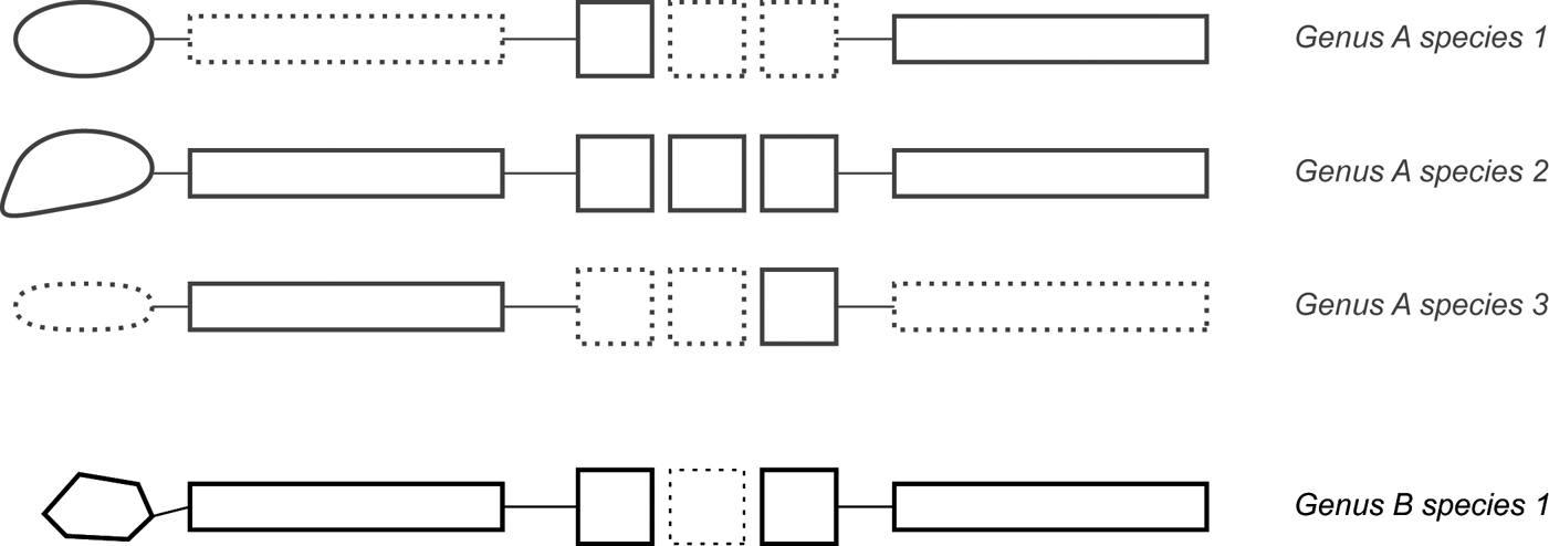
Figure 4 Missing data can reduce pairwise dissimilarity scores to 0 %. Four hypothetical skeletons, where only skull shape (to the left) changes. Rounded skulls are an autapomorphy of genus A, and angled ones an autapomorphy for genus B. Different skull shapes distinguishing species within genus A. Hypothetical, not preserved, elements are marked with dashed lines. In such a simplified case, a skeleton not preserving postcranial elements can still be identified at species level (e.g., Genus A species 1), whereas the incomplete fossil actually belonging to Genus A species 3 does not show any dissimilarities with any species of genera A and B, and can only be referred to a higher-level taxon. Pairwise dissimilarity between this fragmentary specimen and the specimens of the other species would be 0 %.
The distance method was applied by Tschopp et al. (Reference Tschopp, Mateus and Benson2015), who also developed an additional approach, which they termed ‘apomorphy count'. Recovered apomorphies are qualitatively assessed based on their variability within the clade they define, and among the other OTUs. At the level of specimens, recovered ‘autapomorphies' of single specimens are not necessarily species autapomorphies, whereas recovered ‘synapomorphies' of specific clades might actually represent autapomorphic features of a particular species. Single-specimen ‘autapomorphies' are, therefore, especially prone to simply code for intraspecific variability. Consequently, Tschopp et al. (Reference Tschopp, Mateus and Benson2015) excluded recovered ‘autapomorphies' from their counts, if they were shared with other specimens of closely related species (i.e., shown to be homoplastic; Fig. 5). Additionally, Tschopp et al. (Reference Tschopp, Mateus and Benson2015) excluded ‘synapomorphies' from their apomorphy counts, if they were variable within the clade they define, shared with specimens of other clades and found solely by one of the two analyses they performed. Apomorphies considered valid after this step (which could be both ‘autapomorphies' and ‘synapomorphies') are then counted for two branches of a dichotomy, and summed in order to determine the number of major morphological changes between the two. As such, only characters deemed significant enough by the software TNT to be considered apomorphies, and which are not too variable among the ingroup are counted. These apomorphies can also be distributed unequally: in an extreme case, they could all occur on one branch of the dichotomy only, with the sister-group having not a single apomorphic feature. The apomorphy count, therefore, also partially accounts for unequal rates of morphological evolution.

Figure 5 Qualitative assessment of ‘synapomorphies' and ‘autapomorphies' within a specimen-level context, following Tschopp et al. (Reference Tschopp, Mateus and Benson2015). Acronyms with numbers indicate the character states that diagnose particular clades (in the tree), and the hypothetical distribution of these derived states among the ingroup. ‘Synapomorphies' can be unambiguous (U, shared among all members of the clade they diagnose, and only among them), exclusive (E, occur only in specimens belonging to the clade they diagnose, but not in all of the specimens), shared (S, shared among all members of the clade they diagnose, but not only) and ambiguous (A, shared by most members of the clade they diagnose, and also by specimens belonging to other groups). The latter are the most dubious ‘synapomorphies', and probably not all of them should be considered valid. Tschopp et al. (Reference Tschopp, Mateus and Benson2015) did not consider ambiguous ‘synapomorphies' found only by one of their two analyses for the apomorphy count. ‘Autapomorphies' can be unambiguous (U) and ambiguous (A). Ambiguous ‘autapomorphies' shared with specimens in a closely related clade were not counted for the apomorphy count as implemented by Tschopp et al. (Reference Tschopp, Mateus and Benson2015).
Based on earlier taxonomic interpretations of specific and generic distinctions, for which sister-taxon relationships have been confirmed by their specimen-level analysis, Tschopp et al. (Reference Tschopp, Mateus and Benson2015) then defined thresholds for how many significant morphological changes were historically accepted within a species and within a genus, and applied these consistently across their ingroup taxon Diplodocidae. In the latter study, two traditionally recognised species clusters were confirmed by the analysis (Apatosaurus ajax and A. louisae, and Diplodocus carnegii and D. hallorum), and changes between these sister-groups amounted to a maximum of 12, leading Tschopp et al. (Reference Tschopp, Mateus and Benson2015) to use 13 changes as a minimum threshold to justify generic separation. At the species level, a number of specimens historically referred to a single species were found as sister-OTUs by Tschopp et al. (Reference Tschopp, Mateus and Benson2015) as well. Differences between these specimens summed to maximally five, so that six changes were considered as sufficient for justifying specific distinctions (Tschopp et al. Reference Tschopp, Mateus and Benson2015). However, it is important to note that the absolute number of changes depends on the dataset, and can thus not be uniformly applied to any specimen-level phylogenetic analysis. Concerns about this method are the fact that the resulting absolute numbers vary between any single phylogenetic analysis performed, and that highly incomplete specimens are likely to show fewer apomorphic features. Both methods (pairwise dissimilarity and apomorphy counts), in part, take earlier, and well-accepted, interpretations of species and genera as a basis for the definition of the taxonomic thresholds, and thus also include the taxonomical history of a given clade to some extent.
Kimura et al. (Reference Kimura, Flynn and Jacobs2016) proposed a combination of phenetic, ecological and diagnosability criteria to study lineage sorting in murid mammals, based on morphometric and carbon isotope analyses. Although their study was not based on a phylogenetic analysis, these criteria could be easily adapted for use with a cladogram. Interestingly, and thanks to their extensive and stratigraphically well dated data set, Kimura et al. (Reference Kimura, Flynn and Jacobs2016) found that the different species-delimitation thresholds did not occur simultaneously, but that, based on the phenetic criterion, new species could be recognised earlier in geological time than based on the other criteria. This finding correlates well with the interpretation of a species as a lineage, as is the case in the General Lineage Concept (de Queiroz Reference de Queiroz, Howard and Berlocher1998). Based on the assumption that species lineages diverge gradually during the process of speciation, and that they gradually accumulate distinguishing features along the way, different operational criteria (such as the ones used by Kimura et al. Reference Kimura, Flynn and Jacobs2016), can be plotted onto diverging lineages, and evaluated in light of the General Lineage Concept.
Although the studies and approaches mentioned above yielded promising results concerning species delimitation, it remains unclear if the outcomes represent accurate identifications of the boundaries between true biological species. Indeed, populations exist today that are only reproductively isolated due to behavioural incompatibility (e.g., Nanda & Singh Reference Nanda and Singh2012). Although this can obviously not be detected in extinct species, behavioural incompatibility can be a first step during cladogenesis in the context of the General Lineage Concept, followed by morphological distinctiveness due to diverging evolution. While morphologically indistinct, ‘biological species' might be an issue when comparing extinct with extant forms, it is not necessarily a problem when working with fossil taxa alone. What we need to develop are consistent and reproducible studies for taxonomic clustering at the lowest possible level. In palaeontological datasets, this can only be done based on morphological differences. Even if these clusters do not represent exactly true biological species, a use of distance measures or apomorphy counts will produce consistent and objective units that can be counted in diversity studies.
None of the proposed species-delimitation approaches is without problems. In fact, the various competing species-delimitation methods are based on different species concepts (Adams Reference Adams2001; Sites & Marshall Reference Sites and Marshall2004; Kimura et al. Reference Kimura, Flynn and Jacobs2016), and effectively represent the operational ways of how to apply these concepts to recognise species in nature (Adams Reference Adams2001). Given that the numerous species concepts (both theoretical and operational) just define species at different steps of the speciation process (and can, indeed, be united in the General Lineage Concept for species, as proposed by de Queiroz Reference de Queiroz, Howard and Berlocher1998), it is paramount to apply a number of operational criteria to assess species delimitation (Sites & Marshall Reference Sites and Marshall2004; Bacon et al. Reference Bacon, McKenna, Simmons and Wagner2012; Satler et al. Reference Satler, Carstens and Hedin2013). Conflicting outcomes can then be evaluated qualitatively in light of speciation processes, as has been successfully achieved with palaeontological material by Kimura et al. (Reference Kimura, Flynn and Jacobs2016). Such a need for an integrative approach to species delimitation has been confirmed by the results of a case study of fungi by Dettman et al. (Reference Dettman, Jacobson, Turner, Pringle and Taylor2003), where the phylogenetic species recognition approach (based on genetic distance) identified an additional species, which was still able to produce viable offspring with the sister-group. Similarly, generally accepted species of plants exhibited only some of the criteria applied in case studies of palms and Primula, implying that speciation has not yet led to complete lineage sorting in these taxa (Bacon et al. Reference Bacon, McKenna, Simmons and Wagner2012; Schmidt-Lebuhn et al. Reference Schmidt-Lebuhn, de Vos, Keller and Conti2012). These examples of molecular studies and the case study of fossil murids by Kimura et al. (Reference Kimura, Flynn and Jacobs2016) show that by applying different operational concepts to taxa with a good fossil record, it is possible to trace morphological speciation along a phylogenetic tree.
2. Ceratopsian case study
In order to illustrate some of the challenges outlined above, we conducted a case study based on the analysis of Campbell et al. (Reference Campbell, Ryan, Holmes and Schröder-Adams2016) on chasmosaurine ceratopsians, which used a modified version of the matrix of Sampson et al. (Reference Sampson, Loewen, Farke, Roberts, Forster, Smith and Titus2010). Reanalysis of this study is informative, because Campbell et al. (Reference Campbell, Ryan, Holmes and Schröder-Adams2016) did not apply several of the methodological steps outlined herein to address specific challenges. For instance, Campbell et al. (Reference Campbell, Ryan, Holmes and Schröder-Adams2016) treated all multistate characters as unordered and performed the analysis under equal weights (J. Campbell, pers. comm. 2018). They pruned OTUs only a posteriori, as recommended herein, but the deleted taxa were selected based on their amount of missing data rather than their instability in the MPTs. Finally, Campbell et al. (Reference Campbell, Ryan, Holmes and Schröder-Adams2016) delimited species based on a morphometric study of a character of the frill (the variable angle of an embayment on the posterodorsal bar) rather than either the distance measure or apomorphy count approaches outlined previously.
2.1. Methodology
Herein, we treated the multistate characters that appeared to describe clear morphological transitions as ordered (characters 40, 41, 50, 60, 68, 70, 80, 89). Some of these characters had to be rescored to bring the states into the right order to describe a linear transition (characters 40, 41, 50, 70, 80; see supplementary material, available at https://doi.org/10.1017/S1755691018000877). During the analysis with TNT v. 1.1 (Goloboff et al. Reference Goloboff, Carpenter, Arias and Esquivel2008b), we applied an extended implied weighting strategy, with a k-value of 5, and otherwise followed the search strategies of Campbell et al. (Reference Campbell, Ryan, Holmes and Schröder-Adams2016). A second analysis was performed with the original matrix under equal weights, applying only the character ordering, as outlined in Section 1.2.2, and agreement subtree and pruned tree options in TNT in order to assess possible hidden phylogenetic structure in the large polytomy found by Campbell et al. (Reference Campbell, Ryan, Holmes and Schröder-Adams2016, fig. 5a).
Before applying species delimitation methods, we collapsed the nodes with low supports by using tree bisection and reconnection (TBR), as suggested by Goloboff et al. (Reference Goloboff, Torres and Arias2018). We tentatively applied the apomorphy count to the resulting tree as a means of delimiting species. Given that the ingroup just includes two genera, we excluded all ambiguous ‘synapomorphies', and all ambiguous ‘autapomorphies' shared with any other member of the ingroup during the qualitative assessment of the apomorphies found by TNT (the final counts are given in the supplementary material). The apomorphy count had to be slightly adapted because the TBR collapsing resulted in a partly unresolved tree, so that the sums of apomorphies could not always be counted between two branches of a dichotomous node. Therefore, we calculated the average count across all possible sister-group relationships within a polytomy.
2.2. Results
2.2.1. Analysis under extended implied weights
The analysis with ordered multistate characters and under extended implied weights yielded a single, completely resolved phylogenetic tree with a length of 15.69203 (Fig. 6). The only clade of the ingroup recovered by Campbell et al. (Reference Campbell, Ryan, Holmes and Schröder-Adams2016), including the two specimens referred to Vagaceratops irvinensis, is also found here, as part of a larger clade, which also includes the type specimen of Chasmosaurus russelli (CMN 8800; Fig. 6). This entire clade forms the sister group to a clade including the type specimen of C. belli (CMN 0491; Fig. 6). Three specimens are found as successively more basal OTUs to these two clades: ROM 839, CMN 1254 and AMNH FARB 5401, which are the type specimens for C. brevirostris, C. canadensis and C. kaiseni, respectively. All the specimens referred to C. russelli by Campbell et al. (Reference Campbell, Ryan, Holmes and Schröder-Adams2016) are found in the clade with the type specimen of C. belli, whereas the type specimen of C. russelli is found in a clade with two specimens previously referred to C. belli (Fig. 6).
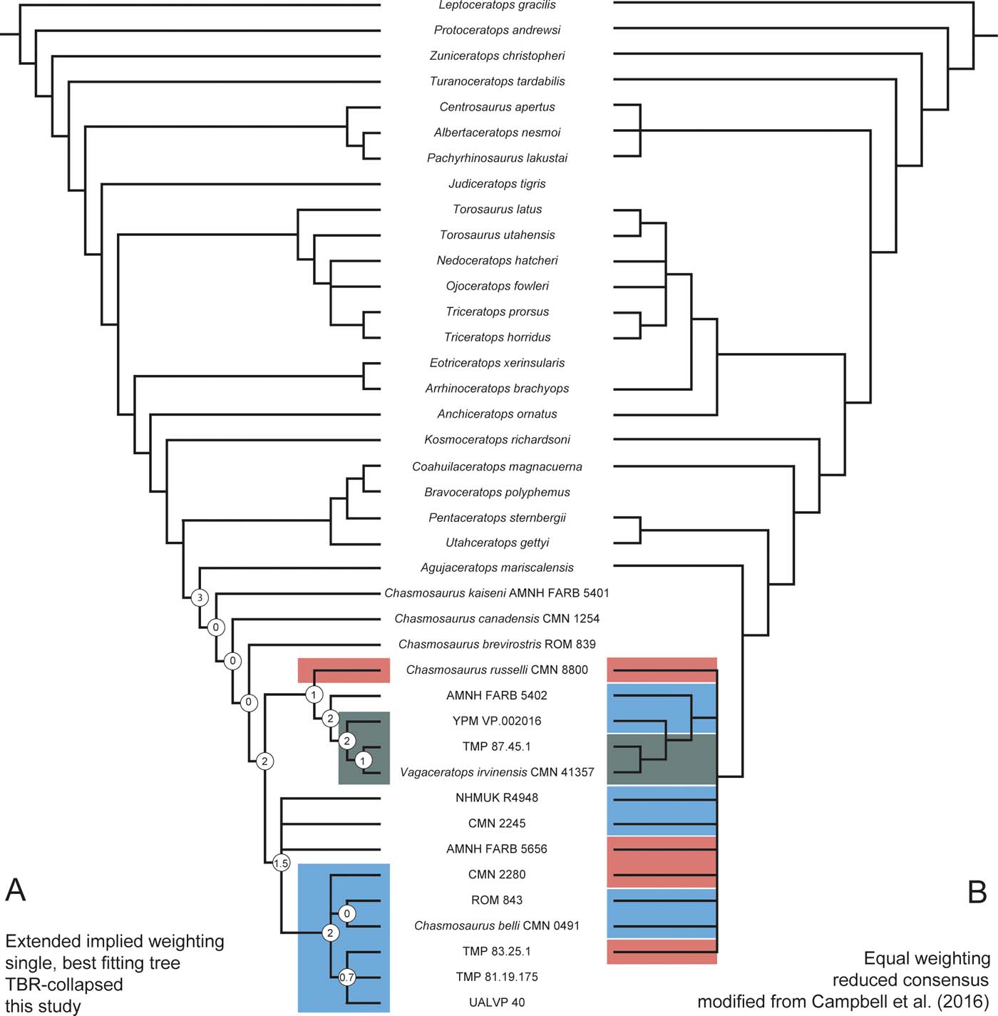
Figure 6 Different weighting strategies lead to conflicting tree topologies in ceratopsian dinosaurs. The tree obtained under extended implied weighting (A) is better resolved than the one under equal weighting (B), modified from Campbell et al. Reference Campbell, Ryan, Holmes and Schröder-Adams2016, even after TBR-collapsing. The systematic referrals of Campbell et al. (Reference Campbell, Ryan, Holmes and Schröder-Adams2016) are contradicted by the apomorphy count applied to the tree obtained using the extended implied weighting approach (see numbers in circles in A). The specimens referred to Chasmosaurus russelli are highlighted in red; specimens referred to C. belli are highlighted in blue; and specimens referred to Vagaceratops irvinensis are highlighted in dark green. Non-highlighted specimens in (A) are specimens with unclear taxonomic assignments (see Sections 2.2 to 2.3).
2.2.2. Analysis under equal weights
The reanalysis of the original matrix provided as supplementary material by Campbell et al. (Reference Campbell, Ryan, Holmes and Schröder-Adams2016) under equal weights, and with ordering of some multistate characters (see list in Section 2.1), yielded more than 30,000 most-parsimonious trees (we only allowed TNT to store 30,000 trees for this preliminary analysis) with a length of 297 steps – four more than reported by Campbell et al. (Reference Campbell, Ryan, Holmes and Schröder-Adams2016) – which is probably a result of the ordering of some of the multistate characters in our analysis.
Our reanalysis found the same large polytomy within Chasmosaurinae as did Campbell et al. (Reference Campbell, Ryan, Holmes and Schröder-Adams2016). Neither the a posteriori pruning processes, as implemented in TNT, nor an agreement subtree revealed more underlying phylogenetic structure.
2.2.3. Apomorphy count
The sums of changes between two branches of a node ranged from zero to three, which is very low compared to those reported by Tschopp et al. (Reference Tschopp, Mateus and Benson2015). However, as pointed out previously, these absolute numbers depend on how a matrix is constructed. As a guideline to subdivide species following historical taxonomic practice, we took the sums of changes between the clades, including the holotypes of the two generally accepted species Chasmosaurus belli and C. russelli, which amounts to two (Fig. 6). For the necessary number to define a genus, we checked the sum of changes between the entire clade attributed to Chasmosaurus and its closest outgroup, Agujaceratops, which corresponds to three. Based on these counts, Vagaceratops irvinensis would only be considered a different species within a paraphyletic C. russelli, and not a distinct genus. However, both nodes along the lineage from C. russelli to V. irvinensis have an apomorphy count of two. A similar condition occurs along the stem of C. belli (Fig. 6). Accepting the General Lineage Concept, these continued, elevated counts might be an indication of gradual morphological change during the speciation process. However, stratigraphic tests would be needed to sustain such a claim. The apomorphy count thus supports the validity of three species within Chasmosaurus, but no distinct genus Vagaceratops.
2.3. Discussion
As shown in Section 2.2.1, the analysis under extended implied weighting recovered a much more resolved tree than the one under equal weights, even after TBR-collapsing. Moreover, most of the referrals by Campbell et al. (Reference Campbell, Ryan, Holmes and Schröder-Adams2016) could not be confirmed based on this tree topology, indicating that the single character proposed as distinguishing the two species Chasmosaurus russelli and C. belli by Campbell et al. (Reference Campbell, Ryan, Holmes and Schröder-Adams2016) might not be taxonomically informative. According to these authors, the two species can be distinguished by the embayment of the posterior parietal bar, which is deep in C. russelli and shallow in C. belli. Although we cannot know the correct phylogenetic tree, our study implies that this character should be assessed in more detail, in particular concerning alternative interpretations such as sexual dimorphism. The latter has already been tentatively suggested by Lehman (Reference Lehman, Carpenter and Currie1990), and might have to be reconsidered given our analysis.
Our results highlight the importance of using different weighting strategies, and a combination of methodological approaches that suit the specific challenges of a specimen-level phylogenetic analysis. However, given that our tests are only preliminary, the underlying causes of the potentially conflicting taxonomic interpretations based on Campbell et al. (Reference Campbell, Ryan, Holmes and Schröder-Adams2016), and the tree recovered herein, are better addressed by experts in chasmosaurine anatomy.
3. Recommendations
Recommendations for the various steps of a specimen-level phylogenetic analysis are collated and summarised in this section. For detailed rationales and case studies, see the discussion in Section 1.
3.1. Matrix construction
Phylogenetic matrices for specimen-level analyses should generally include as many data points as possible. Neither character selection nor OTU sampling should be guided by the amount of missing data. An inclusion of all holotype specimens in the analysis is necessary for systematic reviews. The only justification for a priori exclusion of certain specimens is when they are incomplete, juvenile non-type specimens, which could mislead the analysis because of the typically higher number of plesiomorphic traits in individuals of an early ontogenetic stage.
Character scoring should include approaches to address polymorphisms along the vertebral column and bilateral asymmetry. The most straightforward and promising approaches are frequency or majority scoring for serially variable characters, and the inclusion of an intermediate character state for bilaterally asymmetric traits. Continuous characters can be used, but should be scored with a value representing a central tendency instead of ranges or minimum or maximum values. If juvenile specimens have to be included, they should not be scored for reportedly ontogenetically variable traits. Ordered multistate characters should be represented by their additive binary equivalents in order to reduce the impact of missing data.
3.2. Phylogenetic methodology
Characters should be weighted differentially, using an extended implied weighting approach as implemented in the software TNT with variable k-values. Multistate characters should be treated as ordered if they are quantitative (including continuous characters), or if they describe clear transitions in morphology.
Polytomies in the resulting consensus trees cannot be taken as evidence for species-level clades, but have to be analysed for possible hidden phylogenetic structure by using reduced consensus approaches. At the same time, weakly supported nodes should be collapsed to avoid the recovery of spurious groups. Conflicting topologies recovered after performing the analysis with different weighting constants are best evaluated using a combination of methods (e.g., jackknifing, relative length increases in constrained searches). Additional tests might be based on data extrinsic to the analysis itself, such as stratigraphic or geographic ranges, but this must be stated clearly to avoid circularity in subsequent biostratigraphic or palaeobiogeographic studies.
3.3. Species delimitation
Species delimitation should be carried out based on several approaches, and the differing results assessed from a cautious taxonomic perspective. A combination of tree-based approaches with measures of morphological distance and possibly additional, extrinsic data are expected to provide the most accurate results. However, when using extrinsic data, the same concerns apply here as when testing for accuracy in tree topology (see Section 3.2).
4. Future research
4.1. Validation of the method
As has happened frequently with many other biological and palaeobiological techniques, the development and application of specimen-level morphological phylogenetic methods have proceeded prior to any attempt to validate its accuracy. Validation of the methodologies of morphological specimen-level phylogenetic analyses, using extant taxa, is the first step that should be undertaken. This has been proposed for species delimitation methods by Sites & Marshall (Reference Sites and Marshall2004), and has been carried out using molecular approaches in some fungi and plants (Dettman et al. Reference Dettman, Jacobson, Turner, Pringle and Taylor2003; Bacon et al. Reference Bacon, McKenna, Simmons and Wagner2012). Without such tests, any follow-up study addressing the further potential of specimen-level analyses based on morphology (see Section 4.3) will be flawed and lack a firm methodological base. Extant taxa have to be chosen carefully, and should represent species and genera, where several recent phylogenetic studies based on multiple molecular sequence data confirm at least monophyly of the ingroup. Validation studies should be undertaken for a number of disparate and distantly related clades, in order to assess if the methodology that works best is the same across clades, or has to be adapted for each group of organisms. The studies of Wiens & Penkrot (Reference Wiens and Penkrot2002) on lizards and Dettman et al. (Reference Dettman, Jacobson, Turner, Pringle and Taylor2003) on fungi would suggest the latter: whereas different methodologies led to discordant results in lizards (Wiens & Penkrot Reference Wiens and Penkrot2002), the opposite was the case in fungi (Dettman et al. Reference Dettman, Jacobson, Turner, Pringle and Taylor2003). Thus, a wide survey seems to be necessary to detect significant patterns.
Aside from a general test of whether specimen-level morphological phylogenetic analyses are capable of accurately identifying species among extant taxa, validation and testing is also needed for each of the alternative steps and assumptions available to the researcher. For example, it would be interesting to examine whether the morphological distance approach of Benson et al. (Reference Benson, Evans and Druckenmiller2012) or the apomorphy-based approach of Tschopp et al. (Reference Tschopp, Mateus and Benson2015) yields the most accurate assessments of species delimitations among extant taxa where the ‘correct' answer is already known based on molecular phylogenies or direct field observations of reproductive isolation. Again, it might be that different protocols are variably successful with particular clades or types of organisms, but this has yet to be investigated in any detail.
Simulations are an additional tool to assess methodological issues, but their utility and applicability to a wide taxonomic range depend strongly on study design (Carstens et al. Reference Carstens, Pelletier, Reid and Satler2013). Therefore, validation studies with real morphological data preferably gathered first-hand should be expected to provide more meaningful results. Nevertheless, simulations could prove to be highly useful to model and address the impact of missing data and of the treatment of ontogenetic features on tree topology (see Wiens Reference Wiens2003 and Carballido & Sander Reference Carballido and Sander2014 for examples simulating missing data and the influence of ontogeny, respectively).
4.2. Beyond parsimony
In addition to validation in different taxa, it will also be important to analyse and compare the accuracy and performance of phylogenetic methodologies other than parsimony, such as Bayesian inference, Maximum Likelihood and Network analysis. Bayesian inference has been shown to be a promising tool for specimen-level phylogeny, because it is possible to allow for the recognition of ancestor-descendent pairs (Cau Reference Cau2017). However, there is an ongoing debate on the accuracy of maximum parsimony versus probability-based approaches, in particular regarding the applicable models of character evolution in probability-based approaches when analysing morphological data (e.g., Wright & Hillis Reference Wright and Hillis2014; O'Reilly et al. Reference O'Reilly, Puttick, Parry, Tanner, Tarver, Fleming, Pisani and Donoghue2016; Goloboff et al. Reference Goloboff, Torres and Arias2018; Sansom et al. Reference Sansom, Choate, Keating and Randle2018). Network analysis might represent a promising approach because it is able to recognise patterns of reticulate evolution and horizontal gene or trait transfer (Morrison Reference Morrison2005), which should be expected to be ubiquitous when using individual organisms as OTUs. Comparisons of these different approaches are rare in vertebrate palaeontology, however, so it remains unclear to what extent these methodologies can fulfil their promise. Therefore, we herein concentrated on parsimony approaches, but we note that the entire discussion concerning the interpretation of phylogenetic topology equally applies to trees recovered by means of other methodologies.
4.3. Potential of phenotypic specimen-level phylogeny
Detailed phylogenetic trees of species known from well-dated stratigraphic successions provide the basis for the study of physical drivers of evolution. Where phylogeny is analysed at the level of individual specimens, external factors do not have to be applied to a species as a whole, but can be applied to single individuals or populations, and specific morphological traits. Thus, once validated with extant taxa, specimen-level phylogeny, combined with fine-scale stratigraphic field work and geological studies revealing palaeoenvironmental and palaeoclimatic factors, could yield information concerning morphological trait evolution within (and possibly across) evolutionary lineages through deep time in pre-eminent detail. Such an approach would allow highly localised and detailed correlations with data on environment and climate in the locale where a diagnostic trait first occurred, and can even help to track speciation processes through the accumulation of new morphological traits.
5. Conclusions
Phenotypic specimen-level phylogenetic analysis has a high potential for significant advances in the study of morphological variability, trait evolution and speciation in deep time. However, certain steps during matrix construction, phylogenetic analysis and interpretation of tree topology have to be followed in order to obtain accurate results. These mostly concern the inclusion of as much data as possible to obtain statistical significance, the application of appropriate weighting strategies to reduce the impact of characters possibly simply describing individual variation and the use of a number of complementing approaches to species delimitation, evaluating potentially conflicting results in light of the General Lineage Concept for species. We also highlight the need for validation studies with extant taxa, where the attribution of specimens to a particular species is known a priori, and can be used to infer the best-fitting methodology in a specific taxon.
6. Supplementary material
Supplementary material is available online at https://doi.org/10.1017/S1755691018000877.
7. Acknowledgements
ET has received funding from the European Union's Seventh Framework programme for research and innovation under the Marie Skłodowska-Curie grant agreement no. 609402-2020 researchers: Train to Move (T2M). ET is currently supported by the Theodore Roosevelt Memorial Fund, Division of Paleontology, and Richard Gilder Graduate School, American Museum of Natural History. We thank the Willi Hennig Society for providing the software TNT for free, and Campbell and colleagues for providing their data online as freely accessible supplementary material. Finally, we would like to acknowledge the inspirational role played by Professor Jenny Clack, whose work on tetrapod evolution and the invasion of the land stands as a model of how palaeobiology can revolutionise our understanding of evolutionary patterns and processes. PU is particularly grateful to Jenny for all of her support during his PhD and later career.


