


1. Introduction
Bubbles in yield-stress fluids arise in both geophysical and industrial processes, ranging from bubbling mud pits through aerated chocolate to foamed cement. This fact has stimulated a number of studies, on both individual bubbles and multiple bubbles. The latter has mostly concentrated on the rheological behaviour of these mixtures and especially foamy yield-stress fluids. Kogan et al. (Reference Kogan, Ducloué, Goyon, Chateau, Pitois and Ovarlez2013) generalized a theoretical homogenization framework introduced initially for suspensions of particles in yield-stress fluids (Chateau, Ovarlez & Trung Reference Chateau, Ovarlez and Trung2008) and studied the shear rheology of these materials experimentally. Goyon et al. (Reference Goyon, Bertrand, Pitois and Ovarlez2010) also investigated the drainage of foamy materials induced by shear.
In this study, however, we focus on the static stability of a cloud of bubbles in a yield-stress fluid, which is directly relevant to a large number of applications in which the mixture remains stationary. By ‘stability’, here we mean entrapment of bubbles without motion. The oil and gas industry has long used foamed cements (and drilling fluids) in well construction (Benge, Spangle & Sauer Reference Benge, Spangle and Sauer1982; Ahmed et al. Reference Ahmed, Takach, Khan, Taoutaou, James, Saasen and Godøy2009). Major themes of the investigation of the Deepwater Horizon oil spill (National Commission on the BP Deepwater Horizon Oil Spill and Offshore Drilling 2011) concerned the stability of the foamed slurry downhole, its testing and suitability for this well. In the wider construction industry, both escaping and trapped bubbles can be desirable in cement pastes, either entrained into the slurry during processing or purposefully foamed. Producing an air void system within concrete by inducing rising bubbles helps concrete to become resistant to freeze–thaw cycles, and thus bubble rise in fresh cement paste is of interest (Ley, Folliard & Hover Reference Ley, Folliard and Hover2009).
Our motivation comes from a different process: gas emissions from tailings ponds resulting from oil sand production. In these ponds, fine and mature fluid tailings form stratified layers, which do not appear to consolidate significantly over time scales of many decades. The bulk rheology of this layer exhibits a yield stress (Derakhshandeh Reference Derakhshandeh2016). Anaerobic micro-organisms biodegrade naphtha, producing methane, which can be one of the main sources of gas emission from tailings ponds. Carbon dioxide is also produced (Small et al. Reference Small, Cho, Hashisho and Ulrich2015). In this case, the ideal scenario will be to prevent bubbles from rising, or indeed we might wish to estimate what is a ‘safe’ trapped gas fraction to be held in the pond. Similar mechanisms in geological materials, such as shallow marine deposits, terrestrial sediments and some flooded soils, also lead to the formation of bubbles (Boudreau Reference Boudreau2012).
The motion of an individual bubble in a yield-stress medium has been studied many times with different approaches. Here we use the simplest viscoplastic model, i.e. Bingham fluid, since we are interested in the onset of motion, which is the same for any ‘simple’ yield-stress fluid model (Frigaard Reference Frigaard2019). Tsamopoulos and co-workers (Tsamopoulos et al. Reference Tsamopoulos, Dimakopoulos, Chatzidai, Karapetsas and Pavlidis2008; Dimakopoulos, Pavlidis & Tsamopoulos Reference Dimakopoulos, Pavlidis and Tsamopoulos2013) in a series of papers investigated this problem using different numerical schemes and reported drag coefficients and steady shapes of bubbles for a wide range of effective parameters such as the Reynolds, Bingham and Bond numbers. Experimental studies (Sikorski, Tabuteau & de Bruyn Reference Sikorski, Tabuteau and de Bruyn2009; Lopez, Naccache & de Souza Mendes Reference Lopez, Naccache and de Souza Mendes2018; Pourzahedi, Zare & Frigaard Reference Pourzahedi, Zare and Frigaard2021b) have explored the velocity and shape of air bubbles rising through Carbopol gel, where elasticity of the yield-stress fluid causes a fore–aft asymmetry in the bubble shapes (a teardrop shape). Some analytical models have been developed to capture this phenomenon (Sun et al. Reference Sun, Pan, Zhang, Zhao, Zhao and Wang2020).
Nevertheless, in the subject of the present study, there is little direct numerical or experimental work to describe the onset of motion. The motion onset problem was first formulated mathematically by Dubash & Frigaard (Reference Dubash and Frigaard2004). Very recently, we conducted a systematic study on the yielding of an individual bubble with different shapes and surface tensions (Pourzahedi et al. Reference Pourzahedi, Chaparian, Roustaei and Frigaard2021a). Meanwhile, Chaparian, Wachs & Frigaard (Reference Chaparian, Wachs and Frigaard2018) have demonstrated that a cluster of particles (with bridges of unyielded material that connect the particles together) can be formed when particles are close enough in a yield-stress fluid, which dramatically increases the critical yield number. Koblitz, Lovett & Nikiforakis (Reference Koblitz, Lovett and Nikiforakis2018) have reported the same phenomenon on investigating sedimentation limits in a dilute suspension of rigid particles within a yield-stress fluid.
Here we focus on a cloud of bubbles – also called a ‘swarm of bubbles’ in the literature (Marrucci Reference Marrucci1965; Gummalam & Chhabra Reference Gummalam and Chhabra1987) – and how the bubbles feel their neighbours and interact with each other. We compute the critical yield number for a bubble cloud beyond which the flow is suppressed and explore the different contributing influences. An outline of the paper is as follows. In § 2, we set out the problem and review the key features of the implemented numerical method. The main results are presented in § 3 and conclusions drawn in § 4.
2. Problem statement
2.1. Mathematical formulation
We consider inertialess incompressible bubbly flow of a yield-stress fluid governed by the non-dimensional equation,
 \begin{equation} 0 ={-} \boldsymbol{\nabla} p + \boldsymbol{\nabla} \boldsymbol{\cdot} \boldsymbol{\tau} - \frac{1}{1-\rho} \boldsymbol{e}_g,\quad \text{in}\ \varOmega \setminus \bar{X}, \end{equation}
and the Bingham model,
 \begin{equation}
\left. \begin{array}{ll@{}} \boldsymbol{\tau} = \left( 1 +
\displaystyle{\dfrac{Y}{\Vert\dot{\boldsymbol{\gamma}}\Vert}}
\right) \dot{\boldsymbol{\gamma}} &
\mbox{if and only if}\ \Vert
\boldsymbol{\tau} \Vert > Y, \\[12pt]
\dot{\boldsymbol{\gamma}} = 0 &
\mbox{if and only if}\ \Vert
\boldsymbol{\tau} \Vert \leqslant Y .
\end{array}\right\} \end{equation}
\begin{equation}
\left. \begin{array}{ll@{}} \boldsymbol{\tau} = \left( 1 +
\displaystyle{\dfrac{Y}{\Vert\dot{\boldsymbol{\gamma}}\Vert}}
\right) \dot{\boldsymbol{\gamma}} &
\mbox{if and only if}\ \Vert
\boldsymbol{\tau} \Vert > Y, \\[12pt]
\dot{\boldsymbol{\gamma}} = 0 &
\mbox{if and only if}\ \Vert
\boldsymbol{\tau} \Vert \leqslant Y .
\end{array}\right\} \end{equation}
Here  $p$ is the pressure inside the ambient yield-stress liquid,
  $\boldsymbol {\tau }$ is the deviatoric stress tensor,
  $\rho = \hat {\rho }_b / \hat {\rho }_l$ is the ratio of the bubble density to the liquid density,
  $\boldsymbol {e}_g$ is the basis vector in the gravity direction (vertically downwards) and
  $Y = \hat {\tau }_y / {\rm \Delta} \hat {\rho } \hat {g} \hat {R}$ is the yield number (
 ${\rm \Delta} \hat {\rho } = \hat {\rho }_l - \hat {\rho }_b$). We have scaled the dimensional pressure (
 $\hat {p}$) and the deviatoric stress tensor (
 $\hat {\boldsymbol {\tau }}$) with the buoyancy stress
  $(\hat {\rho }_l - \hat {\rho }_b ) \hat {g} \hat {R}$, and the velocity vector (
 $\hat {\boldsymbol {u}}=(\hat {u},\hat {v})$) with the velocity,
 \begin{equation} \hat{U} = \frac{{\rm \Delta} \hat{\rho} \hat{g} \hat{R}^2}{\hat{\mu}_l}, \end{equation}
which arises from balancing the buoyancy stress with a characteristic viscous stress ( $\hat {\mu }_l \hat {U}/\hat {R}$); here
  $\hat {R}$ is the radius of the monodispersed circular bubbles and
  $\hat {\mu }_l$ the plastic viscosity of the liquid. Quantities with the hat symbol (
  $\hat {\cdot }$ ) are dimensional. In (2.2),
  $\dot {\boldsymbol {\gamma }}$ is the rate-of-strain tensor and
  $\Vert \cdot \Vert$ is the norm associated with the tensor inner product:
 \begin{equation} \boldsymbol{c} \boldsymbol{:} \boldsymbol{d} =\frac{1}{2} \sum_{ij} c_{ij} d_{ij}, \end{equation}
e.g.  $\Vert \boldsymbol {\tau } \Vert = \sqrt {\boldsymbol {\tau } \boldsymbol {:} \boldsymbol {\tau }}$. Note that generally for bubbles
  $\hat {\rho }_b \ll \hat {\rho }_l$, hence in practice
  ${\rm \Delta} \hat {\rho } \approx \hat {\rho }_l$ and
  $\rho \approx 0$. The whole domain (yield-stress fluid and bubbles) is denoted by
  $\varOmega$, the gas fraction by
  $X$ and the bubble surfaces by
  $\partial X$. Hence the bubble area fraction is
  $\phi ={\text {meas}}(X)/{\text {meas}}(\varOmega )$.
On the bubble surfaces ( $\partial X$) the jump in the traction vector is balanced by the surface tension in the normal direction. In the inviscid limit (
 $\hat {\mu }_b \approx 0$), the tangential stress vanishes,
 \begin{equation} (\boldsymbol{\sigma} \boldsymbol{\cdot}\boldsymbol{n} ) \boldsymbol{\cdot} \boldsymbol{t} = 0,\quad \mbox{on}\ \partial X, \end{equation}
and the normal component satisfies
 \begin{equation} {-}p+p_b+(\boldsymbol{\tau} \boldsymbol{\cdot} \boldsymbol{n}) \boldsymbol{\cdot} \boldsymbol{n} = \frac{\gamma}{\kappa},\quad \mbox{on}\ \partial X, \end{equation}
where  $\boldsymbol {\sigma } = -p {\boldsymbol{\mathsf{I}}} + \boldsymbol {\tau }$ is the Cauchy stress tensor,
  $p_b$ is the pressure inside the bubble,
  $\kappa ~(=1)$ is the radius of curvature and
  $\gamma ~(= \hat {\gamma } / {\rm \Delta} \hat {\rho } \hat {g} \hat {R}^2 )$, with
  $\hat {\gamma }$ being the surface tension coefficient. Depending on the application, one might generate significant non-zero tangential stresses through specialized surfactant, e.g. as in Feneuil, Roussel & Pitois (Reference Feneuil, Roussel and Pitois2020), but this is ignored here.
The main aim of our study is to compute the critical value of  $Y$ that separates a stable/static cloud from a moving cloud. Entrapment of particles and bubbles is characteristic of yield-stress fluids. It is intuitive that, on increasing the yield stress (i.e.
  $Y$), an increasing number of bubbles in the cloud will be trapped. Hence, we attain
  $Y_c$, which is the lowest
  $Y$ for which there is no motion.
Following Dubash & Frigaard (Reference Dubash and Frigaard2004) and Pourzahedi et al. (Reference Pourzahedi, Chaparian, Roustaei and Frigaard2021a), the critical yield number is defined and can be computed directly from
 \begin{equation} Y_c \equiv \sup_{\boldsymbol{v} \in \mathcal{V}, \, \boldsymbol{v} \neq 0} \left\{-\frac{\displaystyle \int_{\varOmega \setminus \bar{X}} \boldsymbol{v} \boldsymbol{\cdot} \boldsymbol{e}_g\,\text{d} A}{\displaystyle \int_{\varOmega \setminus \bar{X}} \Vert \dot{\boldsymbol{\gamma}}\left( \boldsymbol{v} \right) \Vert\,\text{d} A} - \frac{\displaystyle \int_{\partial X}\frac{\gamma}{\kappa} \left( \boldsymbol{v} \boldsymbol{\cdot} \boldsymbol{n} \right)\text{d}S}{\displaystyle \int_{\varOmega \setminus \bar{X}} \Vert \dot{\boldsymbol{\gamma}} \left(\boldsymbol{v} \right) \Vert\,\text{d} A}\right\}, \end{equation}
where  $\mathcal {V}$ is the set of admissible velocity fields. As discussed by Pourzahedi et al. (Reference Pourzahedi, Chaparian, Roustaei and Frigaard2021a) for a circular bubble, the surface tension does not change the critical yield number since
  $\gamma /\kappa$ is constant over
  $\partial X$ and the flow is divergence-free; hence the numerator of the second term in (2.7) vanishes. In other words, since the bubble is circular, it is in its equilibrium shape and the only yielding contribution comes from the bubble buoyancy. Hence, in the present study, assuming that the cloud of bubbles consists of circular bubbles, we neglect the surface tension in what follows.
Our objective is to compute  $Y_c(\phi )$ in a meaningful way. Pourzahedi et al. (Reference Pourzahedi, Chaparian, Roustaei and Frigaard2021a) have shown that, for a single circular bubble, the critical yield number is
  $Y_{c,0}=0.1718$ (see figure 1), using both the method of characteristics for a perfectly plastic medium figure 1(a) and computationally using an adaptive augmented Lagrangian scheme figure 1(b). The critical yield number of an individual bubble is the limit of zero volume fraction, i.e.
  $Y_{c,0}=Y_c (\phi \to 0)$.

Figure 1. (a) Slipline solution about a circular bubble (see Chaparian & Tammisola (Reference Chaparian and Tammisola2021) and Pourzahedi et al. (Reference Pourzahedi, Chaparian, Roustaei and Frigaard2021a) for more details). (b) Speed contour  $\vert \boldsymbol {u} \vert$ at
  $Y=0.17$ about a circular bubble.
2.2. Methodology
We perform computations with randomized positions of the circular bubbles in a square box (with periodic conditions applied on horizontal and vertical faces of the domain), the size of which is  $20 \times 20$ (due to scaling, the bubbles’ radii
  $=1$). We handle the bubbles in the numerical simulation by the same method as discussed in detail by Pourzahedi et al. (Reference Pourzahedi, Chaparian, Roustaei and Frigaard2021a). In overview, we use the augmented Lagrangian method coupled with an adaptive finite element method (Roquet & Saramito Reference Roquet and Saramito2003) implemented in FreeFem++ (Hecht Reference Hecht2012) to solve (2.1)–(2.6). The computational procedure has been validated extensively in our previous studies (Chaparian & Frigaard Reference Chaparian and Frigaard2017; Chaparian et al. Reference Chaparian, Izbassarov, De Vita, Brandt and Tammisola2020; Chaparian & Tammisola Reference Chaparian and Tammisola2021; Pourzahedi et al. Reference Pourzahedi, Chaparian, Roustaei and Frigaard2021a), with the mesh adaptivity to capture yield surfaces to high resolution. We calculate
  $p_b$ for each bubble to satisfy incompressibility by using a Lagrange multiplier. Indeed, in the incompressible limit, on the surface of each bubble
  $\int (\boldsymbol {u} \boldsymbol {\cdot } \boldsymbol {n})\,\text {d}S= 0$. Other details of handling the bubbles are explained in Pourzahedi et al. (Reference Pourzahedi, Chaparian, Roustaei and Frigaard2021a). Since we focus on the onset of motion, no deformation strategy for bubble surfaces is implemented in the numerical scheme. In other words, if
  $Y< Y_c$ then the bubbles move and would deform consequently. However, we are not interested in the situations after motion in the present study, so these calculations are not used, i.e. we increase
  $Y$ until there is no motion.
The numerical experiment protocol in the present study is as follows. For a fixed area fraction, based on the size of the computational domain, we calculate the number of bubbles  $N$ (i.e.
  $\phi =N {\rm \pi}/L^2$, with
  $L=20$ here) and randomly assign bubble position. By changing the yield number, we assess the average velocity of the bubbles as a function of
  $Y$ via
 \begin{equation} N {\rm \pi}U_{{avg}} = \int_{\varOmega \setminus \bar{X}} \boldsymbol{u} \boldsymbol{\cdot} \boldsymbol{e}_g\,\text{d}A, \end{equation}
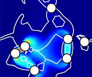
which follows from the continuity equation, i.e. what flows up must flow down. A sample computation at  $\phi =0.055$ and
  $Y=0.25$ is shown in figure 2(a).

Figure 2. (a) Velocity contour at  $Y=0.25$ for a randomized cloud with
  $\phi =0.055$. (b) Average velocity of the bubbles versus the yield number for different realizations (in blue colour with different intensities). Only a few configurations have been shown to avoid cluttering the figure.
Having computed  $U_{{avg}}$ as a function of the yield number (one blue curve in figure 2b), we calculate the
  $Y$ for which the flow stops and hence the critical yield number for the
  $i$th configuration
  $Y_c^i$. We repeat this procedure for other randomized configurations at the same volume fraction. After computing a large number of different configurations, we average the data to approximate
  $Y_c$ for a specific volume fraction:
  $Y_c(\phi ) = (\sum _{i=1}^n Y_c^i)/n$. Note that the computation for each single
  $Y$ for each configuration requires four or five cycles of mesh adaptations. Thus the entire calculation is intensive. We ensure that the number of configurations
  $n$ is enough to reach statistically converged results for the mean (typically
  $n = 25$). We also compute the standard deviation of each sequence of
  $n$ configurations.
The last point to mention is about the size of the periodic box, which is chosen as  $L=20$. We have experimented with different sizes and concluded that
  $L=20$ is sufficiently large to get unbiased data. A larger box could be preferable but we need to compromise, as here the adaptive augmented Lagrangian method is used to capture reliable results at the yield limit, and this is rather exhaustive. It should also be noted that finite size effects are less relevant than for fluids without a yield stress.
3. Results
Following the Monte Carlo procedure described above, the computed critical yield number  $Y_c(\phi )$ is shown in figure 3, represented by the black circles. The error bars mark the minimum and maximum
  $Y_c^i$ obtained in the series of randomized configurations at fixed volume fraction.

Figure 3. Critical yield number versus bubble concentration  $\phi$. The black circle symbols are the randomized cloud bubble simulations results with error bars. The cyan curve is the expression (3.1) and (3.2). The red line marks the single bubble limit,
  $Y_{c,0} = 0.172$. The blue line shows the results obtained from the equally spaced bubbles, as in figure 4. The purple continuous line shows the results obtained from the equally spaced pairs illustrated in figure 6. The dashed purple line shows equally spaced large bubbles of equivalent area to the bubble pairs.
As depicted, the critical yield number increases with the gas volume fraction, which is intuitive. A similar increase has been shown for non-colloidal particle suspensions recently by Koblitz et al. (Reference Koblitz, Lovett and Nikiforakis2018). This increase has two main reasons. Firstly, when the amount of gas increases, a larger yield stress is required to stabilize the mixture. Secondly, as demonstrated by Chaparian et al. (Reference Chaparian, Wachs and Frigaard2018), some networks/clusters of particles can be formed by unyielded bridges, which increase  $Y_c$, since it is no longer individual bubbles/particles that should be brought to a halt by the yield stress; indeed, it is the larger bubble/particle networks that are the last to stop as
  $Y$ is increased.
The increase in  $Y_c$ is linear at low volume fractions, but clearly deviates from linear behaviour at larger
  $\phi$. In our methodology, we have increased
  $Y$ for each configuration until the flow is arrested. In other words, we are increasing the yield stress to reach the critical value. We can represent this as
  $\hat {\tau }_{y,c}(\phi )$:
 \begin{equation} Y_c ( \phi ) = \frac{\hat{\tau}_{y,c} ( \phi )}{{\rm \Delta} \hat{\rho} \hat{g} \hat{R}} = \frac{\hat{\tau}_{y,c} (0)}{{\rm \Delta} \hat{\rho} \hat{g} \hat{R}} \frac{\hat{\tau}_{y,c} ( \phi )}{\hat{\tau}_{y,c} (0)} = Y_{c,0} \frac{\hat{\tau}_{y,c} ( \phi )}{\hat{\tau}_{y,c} (0)} = Y_{c,0}\, f(\phi). \end{equation}
Here  $f(\phi )$ represents the increase in
  $Y_c(\phi )$ over the single bubble
  $Y_{c,0}$. On fitting to the data we find
 \begin{equation} f(\phi) = \frac{\hat{\tau}_{y,c} ( \phi )}{\hat{\tau}_{y,c} (0)} = 1 + 14.49 \phi + 21.26 \frac{\phi^2}{2}, \end{equation}
which is sketched by the broken cyan curve in figure 3. For future reference, the computed data are given in table 1, including the standard deviation.
Table 1. Values of  $Y_c$ and statistics of randomized simulations.

3.1. Further analysis and bounds
Figure 3 contains other curves that shed light on different contributions to the buoyancy–yield stress balance. To get an estimation of the minimal increase in the critical yield number by the increased volume fraction, we simulate the flow around an individual bubble in a periodic box of size  $L_1=\sqrt {{\rm \pi} / \phi }$; see figure 4. In other words, in this simulation, we focus on a bubble suspension in which the bubbles are equally spaced and so the hydrodynamic interactions are minimal compared to the randomized bubble cloud. There are other regular spacings (e.g. hexagonal), but it is reasonable to assume that the in-line arrangement is more likely to yield to motion. The critical yield numbers predicted by these ‘conceptual’ suspensions are shown in blue in figure 3. While, as expected,
  $Y_c$ increases with
  $\phi$ in these simulations as well, the large gap between the blue line and the circle symbols (cloud data) explicitly demonstrates that short-range interactions between the bubbles play an important role in yielding.

Figure 4. Schematic of the equally spaced bubbles with the desired volume fraction and the sample computation at  $Y=0.18$ with
  $\phi =0.055$ (i.e.
  $L_1=7.56$ given that
  $R=1$). The contour shows
  $\vert \boldsymbol {u} \vert$.
For deeper understanding of the short-range interactions, we have revisited a couple of cloud simulations in the dilute regime (mostly at  $\phi =5.5\,\%$). We have found that the critical yield number for the cloud is quite close to
  $Y_c$ of the dominant pair. By ‘dominant pair’, we mean the pair of bubbles that causes high velocity/motion and hence yielding because of their proximity and relative orientation. For instance, for the cloud shown in figure 2(a), the dominant pair is highlighted in red (pair
  $\mathbb {A}$). It is apparent from the velocity contour that the maximum velocity occurs between these bubbles, and this pair is connected by an unyielded bridge. The second dominant pair is highlighted yellow (pair
  $\mathbb {B}$). We perform simulations in which we just model these pairs, ignoring all other bubbles in the cloud and setting
  $\boldsymbol {u}=0$ in the far field. In other words, we simulate the two bubbles that are proximate in an ambient quiescent pool of viscoplastic fluid.
Figures 5(a–d) reveal more flow features (velocity and  $\log (\Vert \dot {\boldsymbol {\gamma }} \Vert )$ fields) around these dominant pairs. Figures 5(a,c) are associated with the pair
  $\mathbb {A}$ and figures 5(b,d) with the pair
  $\mathbb {B}$ extracted from the sample simulation shown in figure 2.

Figure 5. Flow fields around isolated pairs extracted from figure 2. Panels (a,c,e) are associated with the closest pair ( $\mathbb {A}$) and (b,d,f) with the second closest pair (
 $\mathbb {B}$). (a,b) Velocity contours for bubbles; (c,d) contours
  $\log (\Vert \dot {\boldsymbol {\gamma }} \Vert )$ for bubbles; and (e,f) velocity contours around particles; (a,c)
  $Y=0.225$; (b,d)
  $Y=0.2$; (e)
  $Y=0.1425$; and (f)
  $Y=0.17$. Please note that the critical yield numbers for these configurations are: (a,c)
  $Y_c=0.25$; (b,d)
  $Y_c=0.225$; (e)
  $Y_c=0.145$; and (f)
  $Y_c = 0.1725$.
The critical yield number for the cloud shown in figure 2(a) is  $Y_c=0.265$, for the dominant pair (i.e. pair
  $\mathbb {A}$) it is
  $Y_c=0.25$, and for the second dominant pair (i.e. pair
  $\mathbb {B}$) we find
  $Y_c=0.225$. For the sake of conciseness, we do not compare
  $Y_c$ of all the simulated clouds with the dominant pair, but in almost all the cases we have checked that the two critical yield numbers are approximately the same in the dilute regime.
It should be mentioned that generally finding the dominant pair is not trivial and one can easily imagine cases of non-uniqueness or where a larger cluster is dominant. Nor is the dominant pair necessarily the same for bubbles as for solid particles. For instance, figures 5(e,f) show the same arrangements of the pairs ( $\mathbb {A}$ and
  $\mathbb {B}$) when they are solid particles. Interestingly, pair
  $\mathbb {B}$ is the dominant pair in the case of solid particles. Pair
  $\mathbb {B}$ is almost vertically aligned and this triggers the formation of an unyielded bridge between the solid particles, which connects the particles together and increases
  $Y_c$. More precisely, in the case of bubbles, the larger critical yield number is associated with pair
  $\mathbb {A}$ (
 $Y_c=0.25$) whereas, in the case of solid particles, the larger critical yield number is associated with pair
  $\mathbb {B}$ (
 $Y_c=0.1725$). Hence, in different physical problems, the dominant pair could have different configurations. Indeed, it is a multidimensional problem in which proximity and orientation of bubbles/particles are two important parameters.
At higher volume fractions, the whole cloud cannot be reduced to a dominant pair. It is indeed a network of bubbles that controls yielding, and extracting that cluster from a fully packed realization is not trivial. However, to get an estimation, we also investigate another ‘designed’ suspension in which we force each two-bubble pair to have strong short-range interaction by almost touching each other when they are aligned vertically; see figure 6. We again perform simulations in a small periodic box of size  $L_2 = \sqrt {2 {\rm \pi}/\phi }$. The critical yield number of these types of clouds is shown by the purple curve in figure 3. As we see, this leads to an upper bound for the randomized cloud data, since the interactions are forcefully increased. However, if the two touching bubbles are merged to form a larger single bubble of equivalent area, the critical yield number is the dashed purple curve in figure 3, which gives a much smaller
  $Y_c$ because the interactions are absent. It is interesting to note that in this sense bubble coalescence may not be optimal for (onset of) motion! This same procedure could be extended by making the interactions even more dramatic, such as having a vertical chain of three or four touching bubbles instead of two bubbles, presumably with larger upper bounds for
  $Y_c$.

Figure 6. Schematic of the equally spaced twin pairs with the desired volume fraction and the sample computation at  $Y=0.4$ with
  $\phi =0.055$ (i.e.
  $L_2=10.69$ given that
  $R=1$). The contour shows
  $\vert \boldsymbol {u} \vert$.
4. Summary and conclusions
In this study we have focused on clouds of bubbles in a yield-stress fluid and mainly have discussed the critical entrapment conditions of these bubbles. The main objective is to respond to practical problems of environmental or industrial nature: How much gas fraction can be held in a yield-stress fluid? To this end, we performed exhaustive sets of computations with randomized positions of bubbles in a full periodic box and monitored the average velocity of the bubbles as a function of the yield number  $Y$ (i.e. the ratio of the fluid yield stress to the buoyancy stress). The critical yield number that marks the flow/no-flow limit was then extracted for each bubble cloud, and a Monte Carlo procedure was used to determine averaged
  $Y_c$ as a function of gas fraction.
As expected, we found that, for larger volume fractions, the critical yield number is larger. In the dilute regime, the behaviour is linear, but for larger volume fractions, the increase is more drastic. To highlight the different contributions, we also performed simulations for equally spaced suspensions of bubbles, which gives a lower bound to  $Y_c$ due to the larger gas fraction. Computations for vertically aligned twin touching bubbles lead to an upper bound. The short-range interaction of bubbles significantly increases the critical yield number, similar to the formation of clusters in suspension of particles in a yield-stress fluid (Chaparian et al. Reference Chaparian, Wachs and Frigaard2018; Koblitz et al. Reference Koblitz, Lovett and Nikiforakis2018). This fact highlights the importance of computing randomized configurations.
The relevance of randomized distributions is very problem-dependent. In situations where bubbles nucleate within a static fluid, e.g. the oil sands tailings pond application introduced earlier, this is likely to be reasonable, although monosized bubbles are an approximation. Equally, the sensitivity to clustering at higher concentrations is hard to account for, e.g. it may occur due to initial non-uniformity in naphtha concentration. Other bubbly (yield-stress) liquids may be more structured, e.g. in a processing flow. Vigorous shaking of bubbly mixtures can also easily result in non-spherical static bubbles, e.g. see the images in Dubash & Frigaard (Reference Dubash and Frigaard2004). Thus, we are only scratching the surface here. Our work can be, for example, extended to bidispersed/more realistic bubble clouds and also larger  $\phi$. For three-dimensional flows with spherical bubbles, we expect that similar mechanisms and trends would be found, concerning
  $Y_c$, but of course quantitatively different. The main barrier here is to develop fast and effective computational methods. Even with the above, we deal only with a mechanical balance. In a static configuration with
  $Y>Y_c$, diffusive effects of gas solubility may still affect bubble size (i.e. ripening), eventually exceeding our mechanical limits.
Our study includes new perspectives in the study of bubbly flows of yield-stress fluids and even more complex multiphase systems of gels and pastes; the emphasis is on the onset of motion by buoyancy-driven bubbles. In recent years, the knowledge of particle/bubble suspensions in yield-stress fluids has mostly expanded in the rheological studies (Kogan et al. Reference Kogan, Ducloué, Goyon, Chateau, Pitois and Ovarlez2013; Dagois-Bohy et al. Reference Dagois-Bohy, Hormozi, Guazzelli and Pouliquen2015): That is, for a given volume fraction, how is the bulk rheology of the mixture changed? Typically, this results in a multiplicative scaling of the rheological constants. Here we too have such a scaling, captured in  $f(\phi )$; see expression (3.2). Note that the linear increase in
  $f(\phi )$ is much larger than those of rheological closures. The point to emphasize is that there are two quite different considerations: (i) the rheology of a bubbly mixture (with no density difference between phases) when placed under shear, extension, etc.; and (ii) the limit under which buoyancy-driven bubble flows do not occur, studied here for the first time.
Funding
This research was made possible by collaborative research funding from NSERC and COSIA/IOSI (project numbers CRDPJ 537806-18 and IOSI Project 2018-10). This funding is gratefully acknowledged. This computational research was also partly enabled by infrastructure provided from Compute Canada/Calcul Canada (www.computecanada.ca).
Declaration of interests
The authors declare no conflicts of interest.


