
INTRODUCTION
Genotype by environment interaction (G × E) is a common phenomenon in crop production; and remains an important issue in genotype evaluation and recommendation that suits for specific or wider production environments. G × E is understood as the differential ranking of genotypic performances among locations or years. Basically, there are two different approaches towards G × E. The first approach is development of high-yielding genotypes with low G × E interaction; that is, widely adapted genotypes across mega-environments. The second approach is exploitation of G × E by breeding genotypes for maximum yield and stability within mega-environments. Plant breeders conduct multi-environment trials primarily to identify superior cultivars for a target region and to determine mega-environments (Yan et al., Reference Yan, Hunt, Sheng and Szlavnics2000). Targeting of cultivars to specific locations becomes difficult when G × E is present, because yield is less predictable and cannot be interpreted based only on genotypic and environmental means (Ebdon and Gauch, Reference Ebdon and Gauch2002).
Several statistical methodologies have been proposed and employed to analyse and visualize the nature and magnitude of G × E for multi-environment trail data. More recently, however, additive main effect and multiplicative interaction (Gauch, Reference Gauch2006); and genotype plus genotype by environment interaction (GGE) proposed by Yan et al. (Reference Yan, Hunt, Sheng and Szlavnics2000) models are becoming popular for multi-environment trial data analysis. Furthermore, GGE is found to be the best fit for mega-environment analysis (‘which-won-where’ pattern), genotype evaluation (mean vs. stability), and test environment evaluation (discriminating power vs. representativeness) (Yan et al., Reference Yan, Kang, Ma, Wood and Cornelius2007). Several researchers recognized GGE as the most useful method to analyse and visualize the pattern of G × E in multi-environment cultivar evaluation of different crop species, including wheat (Yan et al., Reference Yan, Hunt, Sheng and Szlavnics2000), soybean (Atnaf et al., Reference Atnaf, Kidane, Abadi and Fiseha2013), common beans (González et al., Reference González, Monteagudo, Casquero, De Ron and Santalla2006) and oilseeds (Brar et al., Reference Brar, Singh, Mittal, Singh and Jakhar2010).
White lupin (Lupinus albus L.) is an annual legume crop that is traditionally cultivated around the Mediterranean and along the Nile valley (including Ethiopia) where it is used for human consumption, green manuring and as forage. It is adapted to wide ecological conditions from Alaska to Argentina characterized as low pH, low nutrients availability, high salinity and excess of nitrate (Huyghe, Reference Huyghe1997). In Ethiopia, the crop is mainly grown in northwestern part of the country mainly for its grain and soil maintenance values (Atnaf et al., Reference Atnaf, Tesfaye, Dagne and Wegary2015; Yeheyis et al., Reference Yeheyis, Kijora, Solomon, Anteneh and Peters2010). Several workers evaluated different gene pools of white lupin landraces under different growing environments and have found out that white lupin grain yield and other agronomic and adaptive traits are responsive to different growing conditions, implying the presence of G × E (Annicchiarico and Carroni, Reference Annicchiarico and Carroni2009; Annicchiarico et al., Reference Annicchiarico, Harzic and Carroni2010; González-Andres et al., Reference Gonzalez-Andres, Casquero, San-Pedro and Hernandez-Sanchez2007; Rubio et al., Reference Rubio, Cubero, Martin, Suso and Flores2004). Similarly, region-specific top-yielding (as high as 5 Mg ha−1) white lupin landraces with useful adaptive traits were reported by several investigators in different parts of the world, such as, in Western Europe (Julier et al., Reference Julier, Huyghe, Papineau, Milford, Day, Billot and Mangin1993), Southern Europe (Annicchiarico and Carroni, Reference Annicchiarico and Carroni2009; Annicchiarico et al., Reference Annicchiarico, Harzic and Carroni2010; Rubio et al., Reference Rubio, Cubero, Martin, Suso and Flores2004) and east and north African countries, including Ethiopia, Egypt and Morocco (Atnaf et al., Reference Atnaf, Tesfaye, Dagne and Wegary2015; Christiansen et al., Reference Christiansen, Raza, Jørnsgård, Mahmoud and Ortiz2000; Sbabou et al., Reference Sbabou, Brhada, Alami and Maltouf2010). This indicates specificity in performance and adaptation of the white lupin germplasm considered in those studies. Yeheyis et al. (Reference Yeheyis, Kijora, van Santen and Peters2012) also reported the importance of G × E on the performance of grain yield and other traits in sweet and bitter cultivars of different lupin species evaluated in three different lupin growing locations of Ethiopia. However, no detailed multi-environment evaluation of Ethiopian white lupin has been undertaken so far. The objectives of this work, therefore, were to (i) evaluate the performance and stability of white lupin landraces in different growing environments, and (ii) characterize white lupin growing environments in Ethiopia.
MATERIALS AND METHOD
Study sites
The experiment was conducted at six different locations in northwestern part of Ethiopia; namely, Debre Tabor, Injibara, Merawi, Finote Selam, Dibate and Mandura during the 2014/15 main growing season. The locations represent most lupin growing environments that range from low- to high- altitude agro-ecologies. Detail descriptions of these locations are provided in Supplementary Table S1.
Plant materials
Twelve white lupin landrace accessions were used for the study; of which, eleven (G1, 242281 (Ethiopian Biodiversity Institute, EBI designation); G2, 238996; G3, 238999; G4, 236615; G5, 239029; G6, 239007; G7, 242306; G8, 239003; G9, 239045; G10, 239032; and G11, 207912) were collected and conserved by the EBI from different localities of northwestern Ethiopia and one accession (G12) is a local cultivar commonly grown by farmers in West-Gojam zone.
Experimental design and field management
The experiment was laid out in a randomized complete block design with four replicates, except at Merawi where two replications were used. A plot with an area of 15 m2 (5 × 3 m2) was used. Spacing between plants and rows were 0.25 m and 0.75 m, respectively. The plots were hand planted in rows; and fertilizer was not applied at any of the locations during the cropping period. Agronomic and plant protection management practices were applied uniformly across the plots for the duration of the experiment.
Data collection and analysis
Grain yield data was recorded in grams on plot basis from four harvestable rows and later expressed as mega gram (Mg) per hectare (Mg ha−1) after adjusting moisture content to 14%. The data were subjected to combined analysis of variance employed in the GGE software. The existence of significant G × E variance for grain yield justified further partitioning of the G × E variance into principal components. Partitioning of the G × E was performed using the GGE model. The GGE refers to the genotype main effect and the G × E, which are the two most important sources of variation for cultivar evaluation in multi environment trials (Yan et al., Reference Yan, Kang, Ma, Wood and Cornelius2007). A GGE biplot displays the genotypic main effect and G × E of a genotype by environment dataset (Yan et al., Reference Yan, Hunt, Sheng and Szlavnics2000). This biplot is specially and perfectly used for mega-environment analysis based on genetic correlation between environment and the which-won-where pattern; test environment evaluation based on their discriminating ability and representativeness; and genotype evaluation based on their mean performance and instability within a mega-environment provided that a given data set has a high correlation between PC1 and genotype main effects (Crossa et al., Reference Crossa, Cornelius and Yan2002). This correlation was calculated using the GGE software (Yan, Reference Yan2001). Heritability was calculated on plot bases as proportion of the genotypic variance to the phenotypic variance using the following equation:
 $$\begin{equation}
H = \ \frac{{{\delta_{g}^2}}}{{{\delta_{p}^{2}}}}
\end{equation}$$
$$\begin{equation}
H = \ \frac{{{\delta_{g}^2}}}{{{\delta_{p}^{2}}}}
\end{equation}$$
where H is the broad sense heritability; δ2p and δ2g are phenotypic and genotypic variances, respectively.
The GGE biplot was constructed using the first two principal components (PC1 and PC2) derived from subjecting environment centred yield data (Yan et al., Reference Yan, Hunt, Sheng and Szlavnics2000). The GGE model used was:
 $$\begin{equation}
{Y_{ij}} - \left( {\mu + {\beta _j}} \right) = {\lambda _1}{\xi _{i1}}{\eta _{j1}} + {\lambda _2}{\xi _{i2}}{\eta _{j2}} + {\varepsilon _{ij}}
\end{equation}$$
$$\begin{equation}
{Y_{ij}} - \left( {\mu + {\beta _j}} \right) = {\lambda _1}{\xi _{i1}}{\eta _{j1}} + {\lambda _2}{\xi _{i2}}{\eta _{j2}} + {\varepsilon _{ij}}
\end{equation}$$
where Yij is measured mean of genotype i (=1,2,….,n) in environment j (=1,2…,m), µ is the grand mean, βj is the main effect of environment j, µ + βj being the mean yield across all genotypes in environment j, λ1 and λ2 are the singular values (SV) for the first and second principal component (PC1 and PC2), respectively. ξi1 and ξi2 are eigenvectors of genotype i for PC1 and PC2, respectively. η1j and η2j are eigenvectors of environment j for PC1 and PC2, respectively. εij is the residual associated with genotype i in environment j.
PC1 and PC2 eigenvectors cannot be plotted directly to construct a meaningful biplot before the SV are partitioned into the genotype and environment eigenvectors. SV partitioning was implemented by:
 $$\begin{equation}
{g_{i1}} = \lambda _1^{{f_1}}{\xi _{i1}}\;{\rm{and}}\;\ {e_{ij}} = \lambda _1^{1 - {f_1}}{\eta _{ij}}
\end{equation}$$
$$\begin{equation}
{g_{i1}} = \lambda _1^{{f_1}}{\xi _{i1}}\;{\rm{and}}\;\ {e_{ij}} = \lambda _1^{1 - {f_1}}{\eta _{ij}}
\end{equation}$$
where f 1 is the portion factor for PC1 and can range between 0 and 1. To visualize relationship among genotypes, the GGE biplot based on genotype metric (that is f = 1; S.V.P = 1) and environment metric (f = 0; S.V.P = 2) are appropriate. GGE biplot is important to visualize relationships among environments. So the following equation derived from Equation (2) generates the GGE biplot:
 $$\begin{equation}
{Y_{ij}} - \mu - {\beta _j} = {g_{i1}}{e_{1j}} + {g_{12}}{e_{2j}} + {\varepsilon _{ij}}
\end{equation}$$
$$\begin{equation}
{Y_{ij}} - \mu - {\beta _j} = {g_{i1}}{e_{1j}} + {g_{12}}{e_{2j}} + {\varepsilon _{ij}}
\end{equation}$$
If the data were environment standardized, the common equation to generate the GGE biplot was as follows:
 $$\begin{equation}
\frac{{{Y_{ij}} - \mu - {\beta _j}}}{{{s_j}}} = \sum\nolimits_{i = 1}^k {{g_{i1}}{e_{1j}} + {\varepsilon _{ij}}}
\end{equation}$$
$$\begin{equation}
\frac{{{Y_{ij}} - \mu - {\beta _j}}}{{{s_j}}} = \sum\nolimits_{i = 1}^k {{g_{i1}}{e_{1j}} + {\varepsilon _{ij}}}
\end{equation}$$
where sj is the standard deviation (SD) in environment j, i=1,2,….,k, gi1 and e1j are PC1 scores for genotype i and environment j, respectively. In the present study we used environment standardized model, Equation (5).
RESULTS AND DISCUSSION
Analysis of variance and mean values
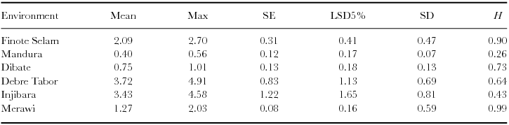
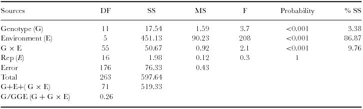
Statistically significant differences were observed among the white lupin genotypes for grain yield at individual locations (Table 1). However, mean performances of the genotypes greatly varied from location to location (Table 2), which might be attributed to differences in test locations for white lupin production. Among the six locations, the highest mean grain yield of 3.72 Mg ha−1 was recorded at Debre Tabor while the lowest (0.40 Mg ha−1) was observed at Mandura. Combined analysis of variance for grain yield over locations exhibited highly significant (p < 0.001) mean squares due to genotype, environment, and G × E among the Ethiopian white lupin landraces (Table 3). Significant variations among the genotypes indicate the differences in the inherent genetic potential of the landraces that makes selection possible, whereas differences among the environments showed the variability in potential suitability of the test locations for white lupin production.
Table 1. Summary statistics for grain yield (Mg ha−1) for individual test locations.

Mg ha−1 = Mega gram per hectare; Landraces = number of landraces; Max = maximum; SE = standard error; LSD5% = least significant difference at 5% probability level; SD = standard deviation; and H = heritability in the broad sense.
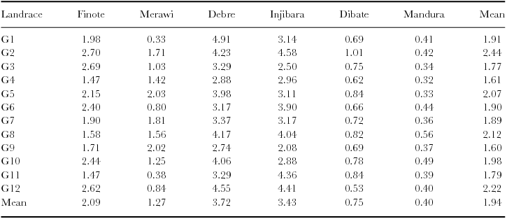
Table 2. Mean grain yield (Mg ha−1) of 12 white lupin landraces tested at six different locations in Ethiopia.

Mg ha−1 = Mega gram per hectare; EBI= Ethiopian Biodiversity Institute; G1-G12 are codes representing white lupin accessions; Finote = Finote Selam; Debre = Debre Tabor.
Table 3. Analysis of variance for grain yield of 12 white lupin landraces grown at six locations in Ethiopia.

G × E = Genotype by environment interaction; Rep (E) = replication nested in each location; G/GGE = ratio of genotype to (genotype plus genotype by environment interaction variance); DF = degree of freedom; SS = sum squares; MS = mean squares; F = F value; % SS = percent sum squares explained.
Before conducting GGE analysis, a basic analysis of variance is useful to get an idea about the relative magnitudes of the various sources of variation. According to Yan (Reference Yan and Yan2014), GGE biplot analysis is suitable whenever G and/or G × E are statistically significant as observed in the current study (Table 3). Annicchiarico et al. (Reference Annicchiarico, Harzic and Carroni2010) and Annicchiarico and Carroni (Reference Annicchiarico and Carroni2009) reported the importance of GGE variances in white lupin grain yield in Italy and France. Across locations, G2 (2.44 Mg ha−1) and G12 (2.22 Mg ha−1) showed higher grain yield, whereas G9 (1.60 Mg ha−1) and G4 (1.61 Mg ha−1) had lower grain yield. Environment effect explained about 86.87% of the total sum of the square, indicating that most of the experimental variations were attributed to the environment. This indicates that the locations were diverse. Of most relevance is the G/(G+G × E) ratio, which is 0.26, indicating that G × E was relatively large in the dataset. This indicates that G × E must be considered in genotype evaluation and that GGE biplot analysis would be essential to reach meaningful conclusions about the genotypes (Yan, Reference Yan and Yan2014).
Larger G × E effect in this study suggests the possible presence of different mega-environments with different winner genotypes (Yan and Kang, Reference Yan and Kang2003). Previous researches indicated the importance of G × E effect in white lupin in Western Europe (Annicchiarico and Carroni, Reference Annicchiarico and Carroni2009) and in narrow leafed lupin in Western Australia and Western Europe (Annicchiarico and Carroni, Reference Annicchiarico and Carroni2009; Bob and Mario, Reference Bob and Mario2003). The present experiment also depicted that the performance of white lupin landraces were different at different testing environments (different winners at different locations) due to the existence of large G × E. The existence of different winner genotypes in different mega-environments complicates the selection process and cultivar recommendation in breeding programmes (Comstock and Moll, Reference Comstock, Moll, Hanson and Robinson1963).
GGE analysis
The present data set showed 0.971 correlations between the primary effects and the genotype main effects which justifies the use of GGE biplot (Crossa et al., Reference Crossa, Cornelius and Yan2002; Yan et al., Reference Yan, Hunt, Sheng and Szlavnics2000). Analysis of principal components showed that the first three PCs had information ratio (IR) >1.0. However, still the first two principal components usually (the 2-D biplot) display the most important patterns (Yan, Reference Yan and Yan2014). Thus, in this study, the first two principal components (PC1 and PC2) of the GGE explained 61.8% (PC1 = 34.3% and PC2 = 27.5%) of the GGE sum of squares using environment standardized model.
White lupin mega-environment analysis in Ethiopia
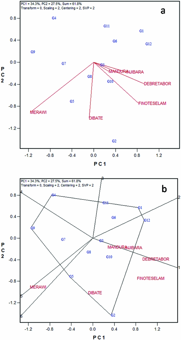
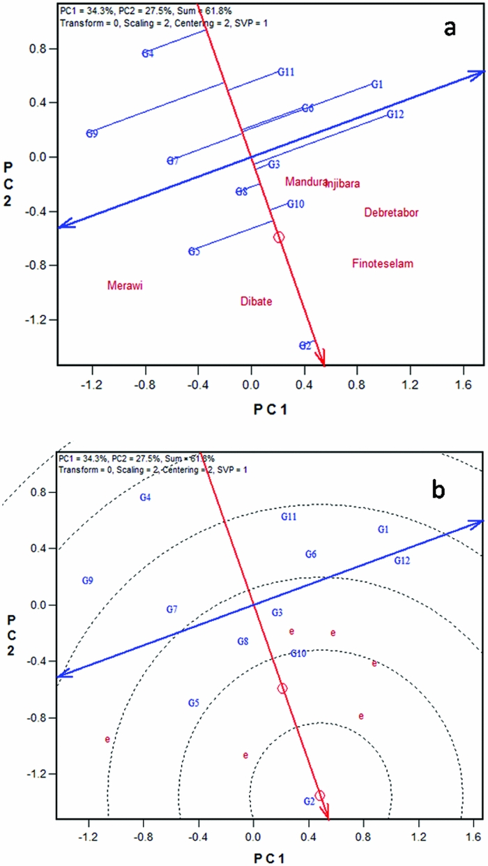
Two forms of the GGE biplot were used in mega-environment analysis; the location vector form (Figure 1a) and the which-won-where form (Figure 1b). The location vector view of the GGE biplot (Figure 1a) facilitates visualization of the genetic correlations between test locations in ranking genotypes based on yield. Lines that connect the biplot origin with environment markers are known as environment vectors and the angle between the vectors of two environments is related to the correlation coefficient between the environments, which is approximated by the cosine of that angle. Acute angles indicate a positive correlation, obtuse and right angles show negative and no correlation, respectively (Yan and Kang, Reference Yan and Kang2003). Five of the six locations used for the current study appeared to be positively correlated. The two high altitude locations, Injibara and Debre Tabor, apparently grouped very close to each other. Two low-altitude locations (Dibate and Mandura) and one mid-altitude location (Finote Selam) were positively correlated. The pattern of relationship among locations generally followed altitudinal and agro-ecological based similarities. The angles between test locations are an indication of the relative magnitude of G versus G × E (Yan, Reference Yan and Yan2014).

Figure 1. White lupin mega-environment analysis based on grain yield data of 12 white lupin landraces evaluated across six locations in Ethiopia employing, (a) location vector view of the GGE biplot, and (b) polygon view of the GGE biplot. G1–G12 are codes for white lupin landraces.
On the other hand, the study showed larger G × E between some locations, for example, strong negative correlation between Merawi and Injibara. The presence of negative correlations among locations suggests that the target region may consist of different mega-environments. The grouping pattern observed in this study suggests that there are two white lupin mega-environments in northwestern Ethiopia (Figure 1a). The first one was high-altitude mega-environment represented by Injibara and Debre Tabor; and the second one was mid- to low-altitude locations that include Finote Selam, Mandura, Dibate and Merawi. However, to confirm patterns observed in the current study, there should be a multi-years data to see the repeatability of the pattern over the years.
Mega-environments are often defined by the which-won-where patterns (Yan et al., Reference Yan, Hunt, Sheng and Szlavnics2000). Visualization of the ‘which-won-where’ pattern in the polygon view is helpful to estimate possible existence of different mega-environments in the target environment (Yan and Rajcan, Reference Yan and Rajcan2002; Yan et al., Reference Yan, Hunt, Sheng and Szlavnics2000). The polygon was drawn on genotypes placed away from the biplot origin so that all genotypes are contained in the polygon. The perpendicular lines radiating from the origin of the biplot divide the biplot area as well as the test locations into sectors. Figure 1b presents a polygon view of twelve white lupin landraces tested at six different locations in Ethiopia. In the biplot, the six locations fell into three sectors. The first sector was marked by radiate lines 1 and 2, where the two high-altitude locations (Injibara and Debre Tabor) fell in. Landrace (G12), a local cultivar obtained from West-Gojam zone, was the vertex genotype in this sector and hence the nominal winner genotype in these locations. This is consistent with mean performance of the cultivar in these locations (Table 2); G12 showed higher grain yield at Injibara and Debre Tabor. The cultivar generally took longer to mature (data not shown) and hence showed better performance in the highland locations with longer growing season. It is generally agreed among the crop experts that earlier maturing genotype, owing to its shorter life cycle, is predisposed to lower yields than a later maturing genotype which has the opportunity to draw nutrients and photosynthesize over a longer period. Several workers documented that white lupin germplasm pools with taller stature, more leaves and branches on the main axis and late flowering and maturity tended to give more yield in environments offering longer growing durations (Annicchiarico and Carroni, Reference Annicchiarico and Carroni2009; Annicchiarico et al., Reference Annicchiarico, Harzic and Carroni2010; Kurlovich, Reference Kurlovich2002; Rubio et al., Reference Rubio, Cubero, Martin, Suso and Flores2004), which exactly agrees with the present finding. The second sector was defined by the radiate lines 1 and 6 (Figure 1b). Low- to mid-altitude locations (Mandura, Dibate and Finote Selam) fell in it, and the landrace (G2) was on the vertex for this sector, suggesting that G2 was the nominal winner at these locations. The third sector was delineated by radiate 5 and 6 and contained only a single location, Merawi; but no genotype fell in the sector.
Results of this study depicted the existence of three white lupin mega-environments in northwestern Ethiopia. However, the third sector in which Merawi fell in (without any genotype) is not distinctively different from the second sector, which contains locations with low to mid attitude. Lack of clear mega-environment classification might be attributed to the fact that the biplots of the present data explained only 63% of the variation. Furthermore, the polygon view of GGE biplot is not consistent with the results of the location vector, which suggested two mega-environments. Above all, it is important to note that conclusions from mega-environment analysis have a long-term effect on breeding and cultivar recommendation and must be based on multiyear data (Yan, Reference Yan and Yan2014); and both the location vector view and the ‘which-won-where’ forms of the GGE biplot (Figure 1) for mega-environment delineations are useful and should be used complementarily.
Mean and stability of white lupin landraces
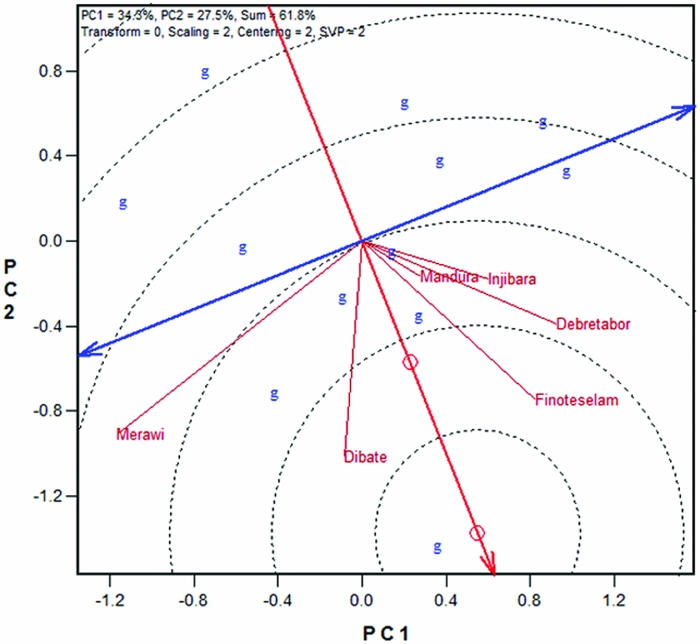
To identify widely adapted landraces, the Mean vs. Instability form of the GGE biplot containing all test locations were used (Figure 2a). In the biplot, the average environment is indicated by the small circle, which is a virtual environment defined by the average coordinates of all the locations to represent the target environment. The line passing through the biplot origin is called the average environment axis (AEA) (Yan and Kang, Reference Yan and Kang2003). The double arrow line, which is perpendicular to AEA and passes through the origin, is termed as average environment coordination (AEC) in which the arrows point to higher instability for the genotypes (i.e., greater contribution to G × E) regardless of the direction. In the present data set, all locations were placed on the same side of the AEC, as shown in Figure 2a, indicating that the G/G × E is sizable and that the AEA is meaningful for genotype evaluation.

Figure 2. White lupin landrace multi location evaluations using (a) the mean versus instability view of the GGE biplot, and (b) ranking landraces based on both mean and instability. G1–G12 are codes for white lupin landraces.
Thus, the landrace G2 has the longest positive projection, indicating that it had the highest mean yield across locations; whereas G4 has the longest negative projection onto AEA, indicating that it had the lowest mean yield across locations. All other landraces were ordered between these two extremes (Figure 2a). The landraces G12 and G3, for example, have projections near the origin on the AEA and had mean yields close to the grand mean of the trial. With regard to stability, length of a line drawn from each genotype onto the AEC indicates instability of the genotype or its contribution to G × E. Hence, G2 contributed little to G × E and therefore was stable, whereas landraces like G12, G1 and G9 contributed more to G × E and were unstable. Annicchiarico and Carroni (Reference Annicchiarico and Carroni2009) reported both specific and wide adapted white lupin cultivars tested in climatically contrasting environments in Italy. Similarly, Annicchiarico et al. (Reference Annicchiarico, Harzic and Carroni2010) reported that germplasm pools from Madeira and Canaries tended to adapt to wider environments whereas others from Europe, east Africa, west Asia and the Mediterranean adapted to specific growing environments in Italy and France.
An ideal genotype should have the highest possible mean performance and be absolutely stable (i.e., contributes zero to the G × E) (Yan and Kang, Reference Yan and Kang2003). This ideal genotype is defined by the small circle in Figure 2b. The desirability of the genotypes is judged by their closeness to this ‘ideal’ genotype. Thus, G2 was the most desirable whereas G4 was the least desirable genotypes in this study. Other landraces based on distance from the ideal genotype were ranked as G10>G5>G8>G3>G12>G7>G6>G1>G11>G9, indicating that those ranked last were less desirable as they were further from the ideal genotype. The distances of genotypes from the ideal genotype (GGE distances) as well as their ranks relative to the ideal genotype are presented in Supplementary Table S2. The smaller the distance of a genotype from the ideal genotype, the more desirable it is.
White lupin test locations evaluation in Ethiopia
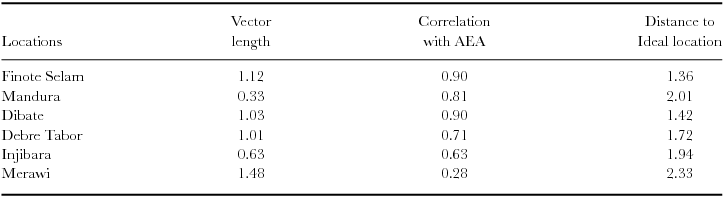
Figure 3 presents the representativeness and discriminative power of white lupin test locations in Ethiopia based on SD-scaled and heritability (h)-weighted data, which is an appropriate biplot for test location evaluation (Yan and Holland, Reference Yan and Holland2010). In the biplot (Figure 3) and Table 4, it was appeared that all locations showed positive correlations with the AEA, and hence all locations were representative. However, the degree of representativeness differs in that Finote Selam and Dibate were most representative white lupin growing locations in northwestern Ethiopia whereas Merawi was the least representative. The length of the location vectors approximates the h of the locations, which is a measure of the discriminating power of the locations. All locations, except Mandura and Injibara, had generally similar and good discriminating power (Figure 3; Table 4). The circle at the centre of the concentric circles represents the ‘ideal test location’ (Figure 3) and it is a virtual location defined to have the longest vector of all locations and to be absolutely representative (i.e., it has zero contribution to G × E and therefore is located on the AEA). The closer a location to this ideal location, the more desirable it is as test location. The concentric circles help visualize this distance. In the biplot, locations Finote Selam and Dibate were closest to the ideal location. Meanwhile, it was observed that locations were not redundant and hence provided different information about the performance of white lupin landraces. Nevertheless, test locations evaluation should be concluded based on multi-years data (Yan, Reference Yan and Yan2014). An ‘ideal test environment should be both discriminating of the genotypes and representative of the mega-environment (Yan et al., Reference Yan, Kang, Ma, Wood and Cornelius2007).

Figure 3. Representativeness and discriminative power of white lupin test locations in Ethiopia.
Table 4. White lupin test locations and genotype by environment statistics.

AEA = Average environment axis.
CONCLUSION
G × E is an important factor in genotype evaluation and recommendation of varieties that are suitable for specific or wider production environments. The GGE biplots are effective enough to analyse and visualize pattern of G × E. Results of the present study depicted differential performance of white lupin landraces at different test environments implying crossover interactions. The results suggested two white lupin mega-environments in northwestern Ethiopia. Finote Selam and Dibate were most representative locations; and all locations, except Mandura and Injibara, had generally similar and good discriminating power for white lupin landraces. Finote Selam and Dibate combined both representativeness and discriminating power and characterized as desirable test locations for white lupin improvement in northwestern Ethiopia. However, mega-environment delineation and test location evaluation should be concluded based on multi-years data over environments. G2 was found to be the highest yielding and most stable landrace across the test environments. Hence, it is the most desirable genotype to be directly recommended for farmers’ use and/or to be used as a source material for future white lupin breeding that targets high yielding and stable genotypes. Findings of this study provide useful information for white lupin breeding and commercialization in Ethiopia.
Acknowledgements
The study was part of PhD research work of the first author (MA). It was financially supported by the Ethiopian Institute of Agricultural Research and Pawe Research Center through Sustainable Intensification of Maize-Legume Systems for Food Security in Eastern and Southern Africa (SIMLESA) project funded by the Australian Government. Provision of experimental land and office facilities by the Amhara Regional Agricultural Research Institute is also highly appreciated. The cooperation and understanding of researchers at each testing location during the whole period of the field experiment (specifically, Desalew at Finote Selam, Zewdu and Abunu at Debre Tabor, Gizachew and Adissu at Dibate) were tremendous and are highly appreciated.
SUPPLEMENTARY MATERIAL
To view supplementary material for this article, please visit https://doi.org/10.1017/S0014479717000515