I. Introduction
State and local government expenditures have been increasing over time in the United States. With this growth in expenditures, there has been an increasing need for tax revenue generation by state governments. States revenues come primarily from sales, property, and income taxes. The increasing need for further revenue generation and voter opposition to the prospect of further increasing broad-based taxes has led state and local governments to search for other sources of revenue collection.
As a popular choice, state and local governments have started to selectively tax goods that pose negative externalities or are considered “sinful.” For such goods, they levy “sin taxes.” Sin taxes are one form of an excise tax. The intention of this tax is to increase revenue and, by increasing the after-tax price of the good, reduce negative externalities that these goods impose. Hence, excise taxes could be assumed to be set high if the primary goal is revenue generation and negative externality reduction. Such goods include tobacco, alcohol, and motor fuels, historically, and more recently, goods such as foods that are high in sugar and trans fat, to name a few (Hoffer, Shughart, and Thomas, Reference Hoffer, Shughart and Thomas2014).
However, when one such good is studied in detail—alcohol, and more specifically, wine, there has only been a 5-cent increase in excise taxes in an 18-year time period. This poses a question as to why there is such a small increase in excise tax if the main goal is to increase revenue and to decrease negative externality. The reason might be because of wine special interest groups furthering their own interests by keeping the excise tax of wine low.
I chose the alcohol industry, and specifically the wine industry for two reasons. First, even though the United States taxed wine as early as 1631 (Sumner, Reference Sumner1892; Hines, Reference Hines2007), it is a fairly new industry in terms of mass production. Second, it is growing in terms of exports, imports, and consumption, and has the potential to increase revenue in the future, making it an important industry to study.
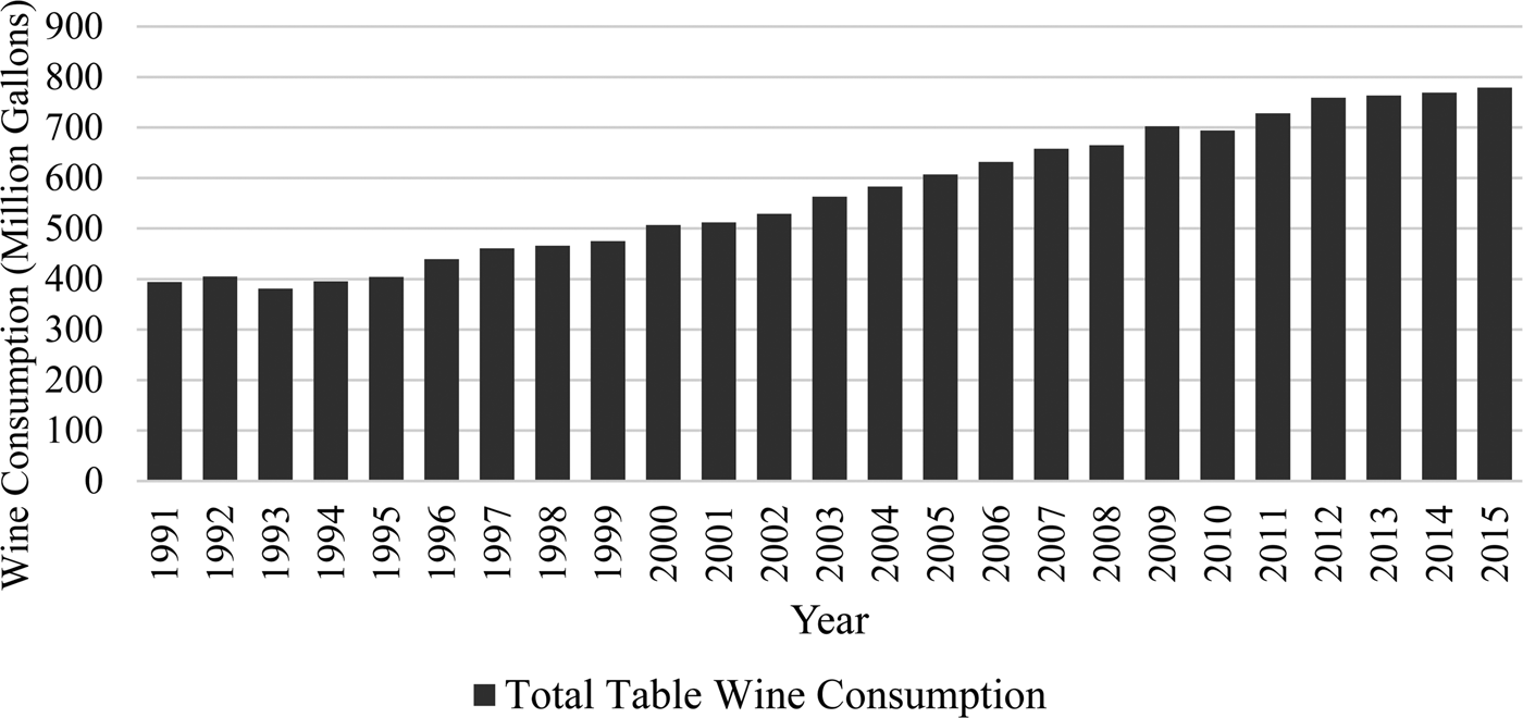
The United States was the seventh largest exporter and the fourth largest producer of wine in 2012. In 2009, the United States accounted for approximately 10% of the world's wine production (Thornton, Reference Thornton2013). Approximately 14% of the world's export volume came from U.S.-produced wine (Anderson and Nelgen, Reference Anderson and Nelgen2011). A report published by MKF Research LLC claims that wineries are now present in all 50 states with $11.4 billion in winery sales revenue.Footnote 1 In North Carolina alone, there are 44 new wineries and 1,000 acres of vineyards as tobacco acreage declined overtime (MKF Research LLC, 2007). Figure 1 shows an almost doubling of total table wine consumption in the United States from 1991–2015, which increased from a little less than 400 million gallons in 1991 to about 800 million gallons in 2015 (Wine Institute, 2016). It represents a huge portion of total wine consumption each year, where total wine consumption increased from 450 million gallons in 1991 to approximately 900 million gallons in 2015 (Wine Institute, 2016).

Figure 1 Wine Consumption in the United States from 1991–2015
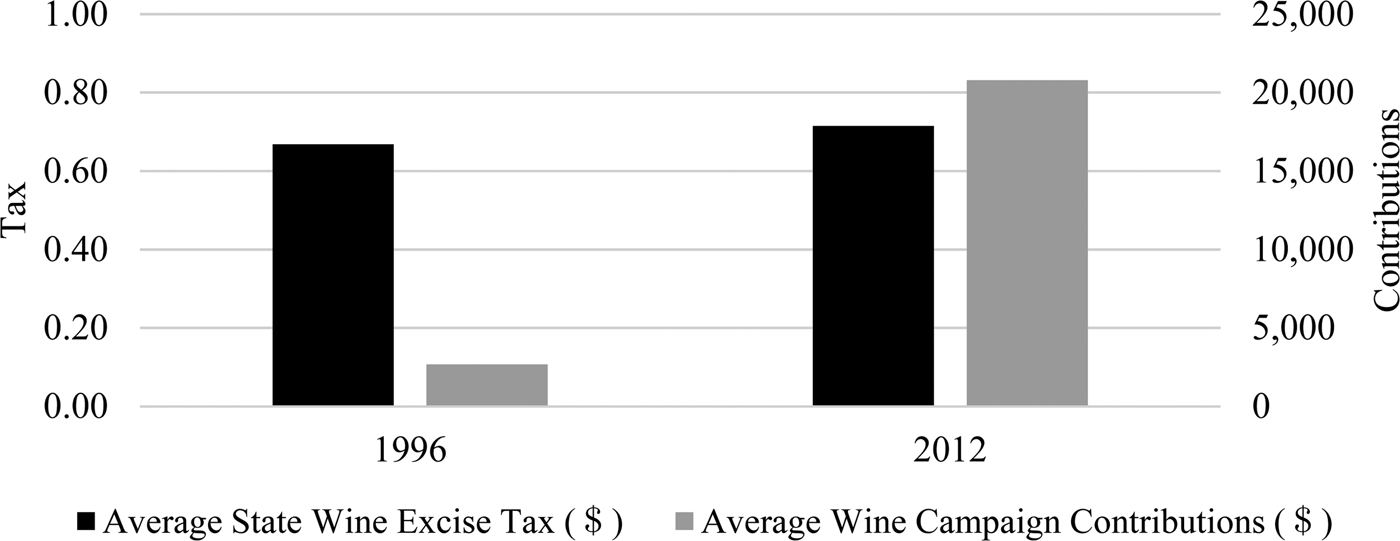
Figure 2 shows average state wine excise tax in years 1996 and 2012. This is indicated by the color black in the figure. Average wine contributions from the wine industry to officials running for state offices for the same years is shown in grey. While the average state excise tax increase was only approximately 5-cents or 7.5% over the course of 18 years, the average dollar amount of campaign contributions has increased by more than 700% in the same 18-year time period. In this context, scholars such as Snyder, Jr. (Reference Snyder1990) and Prat (Reference Prat2002) have looked at campaign contributions as investments. Additionally, Becker (Reference Becker1983, p. 372) wrote:
Political influence is not simply fixed by the political process, but can be expanded by expenditures of time and money on campaign contributions, political advertising, and in other ways that exert political pressure.

Figure 2 State Wine Excise Taxes and Wine Contributions from the Wine Industry to Officials Running for State Offices for an 18-Year Time Period
In terms of special interest group influences, previous studies have looked at the tobacco industry. Holcombe (Reference Holcombe1997) and Hoffer (Reference Hoffer2016) found tobacco special interest to negatively influence tobacco excise taxes, while Besley and Rosen (Reference Besley and Rosen1998), Devereux, Lockwood, and Redoano (Reference Devereux, Lockwood and Redoano2007), and Fredriksson and Mamun (Reference Fredriksson and Mamun2008), found little to no impact of tobacco special interest on tobacco excise tax rates. Studies have also looked at alcohol taxes (taxes on beer, spirits, and wine) on economic outcomes such as pricing (MacDonald, Reference MacDonald1986; Nelson, Reference Nelson1990; Sass and Saurman, Reference Sass and Saurman1996), consumption behaviors and health outcomes (Fell et al., Reference Fell, Fisher, Voas, Blackman and Tippetts2009; Miron and Tetelbaum, Reference Miron and Tetelbaum2009; Elder et al., Reference Elder, Lawrence, Ferguson, Naimi, Brewer, Chattopadhyay, Toomey and Fielding2010). Except for Hoffer (Reference Hoffer2016), these studies do not take into account the spatial dependency in tax rates between states.
In studies of tax rates, there are theoretical and empirical reasons to believe that these rates are spatially correlated. Theoretically, inferences can be made based on Tiebout (Reference Tiebout1956) and yardstick competition (Brueckner and Saavedra, Reference Brueckner and Saavedra2001). Empirically, recent literature has shown that tax rates are interdependent (Deskins and Hill, Reference Deskins and Hill2010) primarily because of the mobility of tax bases (Brueckner, Reference Brueckner2003). For example, wine sellers compete with each other for consumers. Since consumers vote with their feet, consumers straddling state borders for cheaper wine is not uncommon. States establishing wine taxes as a function of neighbor's tax rates is, then, not a surprising outcome. With respect to this study, the data follow a spatial pattern as well. For instance, Missouri increased its wine excise tax from 36 cents in 2000 to 42 cents in 2004. Arkansas increased its tax from 75 cents in 2008 to 77 cents in 2010. At the same time, Mississippi also increased its tax rate from 35 cents to 43 cents. Tennessee increased its tax rate from $1.215 in 2010 to $1.27 in 2012.
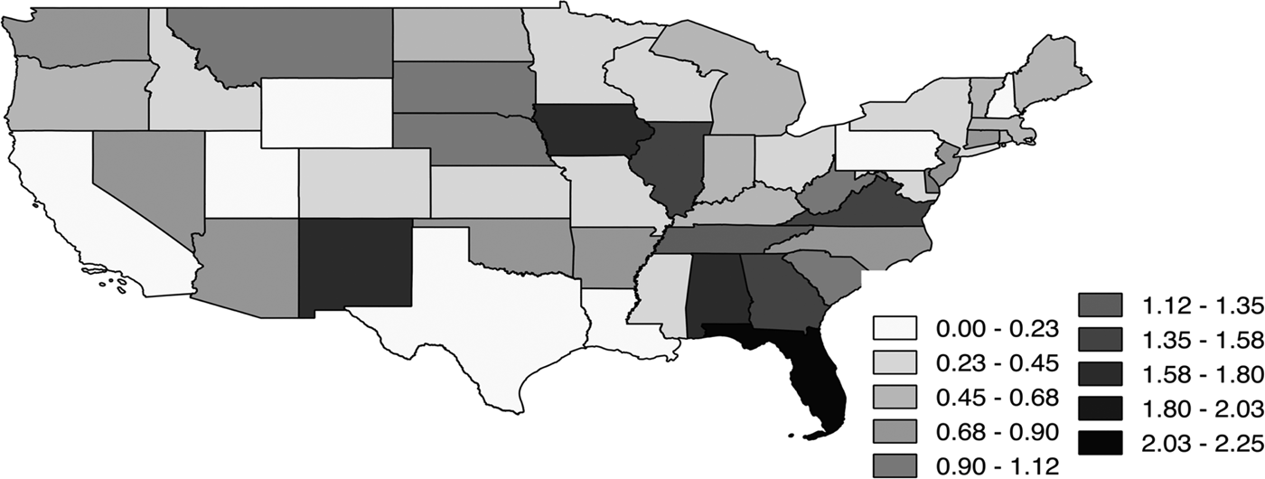
Leaving spatial dependency out of the equation would ignore a possible explanation as to why there is a difference among wine excise taxes between states. While growing need for government expenditure leads to the need for additional revenue generation (Hoffer, Reference Hoffer2016), tax competition points towards higher taxes in neighboring states (Deskins and Hill, Reference Deskins and Hill2010). Following this logic, one should see higher taxes everywhere. However, this is not seen in practice. There is a huge variance among wine excise taxes within U.S. states, with the highest in Florida with $2.25 per gallon in 2012 to the lowest of 0 cents per gallon in New Hampshire, Pennsylvania, Utah, and Wyoming. Figure 3 depicts the differences in wine excise tax rates among the 48 contiguous U.S. states in 2012.

Figure 3 Wine Excise Taxes 48 Contiguous U.S. States in 2012
In this study, I hypothesize that state wine excise taxes are spatially dependent. I employ the Spatial Durbin Model (SDM) to test my hypothesis and find strong statistical evidence that there is spatial dependency in wine excise tax rates between states. I find that higher campaign contributions from the wine industry in a state is negatively associated with wine excise tax in both the given state and its neighbors.
There are two contributions of this article. First, it is the first study to account for the effect of campaign contributions in the alcohol industry, specifically, the wine industry. Previously, studies used total production as a proxy for special interest groups in the tobacco industry (Holcombe, Reference Holcombe1997; Hoffer, Reference Hoffer2016). Second, it is also the first study that looks at the wine industry using a spatial econometric framework. Since I account for spatial dependence, I capture the “spillover” effects or neighborhood effects of changes in the explanatory variables, which would have not been captured had spatial dependence not been accounted for.
The remainder of the article proceeds as follows. Section 2 describes the data and empirical approach used in this study. Section 3 describes the results and Section 4 concludes.
II. Data and Empirical Approach
In this study, I follow Hoffer (Reference Hoffer2016), who looks at the tobacco excise taxes. Instead, I employ state wine excise tax as the dependent variable. The dependent variable is state wine excise tax rate per gallon for the 48 contiguous U.S. states from 1996–2012.Footnote 2 Data on wine excise taxes is obtained from the Distilled Spirits Council of the United States, Inc., the World Tax Database, and the Tax Foundation. According to the Tax Foundation, wine excise tax “rates are those applicable to off-premise sales of 11% ABV non–carbonated 750 mL containers” which are imported from outside the state (Jordan and Drenkard, Reference Jordan and Drenkard2015). In other words, wine excise tax rate is applicable to retail store sales and not to wine sales in restaurants. For example, Florida has a wine tax rate of $2.25. This means that for every gallon of wine bought at an “off-premise” site in Florida, a consumer pays $2.25 in excise taxes.
There are three categories of explanatory variables used in this study that are likely to affect wine excise tax rates: Primary Variables, State Controls, and Demographic Controls. Wine and Beer fall under the Primary Variables category and represent the major variables of interest. Wine proxies for wine-industry special interest in a state while Beer proxies for beer-industry special interest in a state. Wine is the author's calculation and is defined as the dollar amount of wine-industry campaign contribution to officials running for state offices per 100 state residents. For example, campaign contribution from the wine industry to officials running for state offices in California in 2012 was $1.04 per 100 residents. This amounts to approximately $400,000 in campaign contributions just for the state of California in a year.
Since wine and beer can be thought of as substitutes, Beer is used to control for any substitution effects and represents the dollar amount of beer-industry campaign contribution to officials running for state offices per 100 residents.Footnote 3 Beer variable is also the author's calculation. Both Wine and Beer are obtained from the National Institute on Money in State Politics and are inflation-adjusted to 2010 dollars. Contributions from both individuals and non-individuals (business owners, companies, or persons, for instance) are included in the contributions data by the National Institute on Money in State Politics.
In addition to the primary variables of interest, there are other state-government specific variables that fall under the State Controls category that are likely to affect wine excise taxes. There are four variables under this category—Gov_Term, Citizen, Growth_Rate, and Health. Gov_Term, Citizen, and Health are drawn primarily from special interest group literature, specifically, the tobacco special interest literature. I draw from the tobacco special interest literature as, to my knowledge, there are no studies on wine special interests.
Gov_Term represents a dummy variable with a value of 1 if the incumbent governor cannot again run for office due to a term limit and 0 otherwise. If the incumbent governor wins an election, there is a possibility of an increase in wine taxes due to various factors such as demand for revenue. This could act as an incentive for the wine industry to give more in campaign contributions. Hoffer (Reference Hoffer2016) finds a positive relationship between governor term limit and cigarette tax rates. Data for this variable is obtained from The Council of State Governments.
Citizen measures citizen ideology. It is a composite measure that intends to capture electorate sentiment based on ideological measures of the electorate's state elected officials and congressional officials. The notion behind this measure is that electorate ideologies are close to their elected officials. Its score ranges from 1 to 100, where 1 represents “most conservative” and 100 represents “most liberal.” It can be hypothesized that states with more “liberal” citizens would be accepting of higher taxes due to the belief of a more involved role of government. Hoffer and Pellillo (Reference Hoffer and Pellillo2012) find a positive relationship between citizen ideology and tobacco control funding. Yakovlev and Guessford (Reference Yakovlev and Guessford2013) find an ambiguous relationship between political ideology and alcohol consumption. Citizen is obtained from Berry et al. (Reference Berry, Fording, Ringquist, Hanson and Klarner2010) and the measure used is the “revised 1960–2013 citizen ideology series” (Berry et al., Reference Berry, Fording, Ringquist, Hanson and Klarner2010).Footnote 4
Growth_Rate represents the two-year growth rate in state spending. States under fiscal stress could be hypothesized to have a high demand for revenue, thus having a positive relationship with excise taxes. Data for Growth_Rate comes from The Council of State Governments. Health represents the dollar amount per capita spent by states on health expenditures. It is found to negatively affect cigarette excise taxes (Hoffer, Reference Hoffer2016).Footnote 5 Health is obtained from the U.S. Census Bureau.
Additionally, demographic controls are included in order to control for the demographic characteristics of a state's population. Under the Demographic Controls category, there are two variables—Pop65 and PopWhite—that might affect state wine excise taxes in terms of population tastes for wine. Pop65 represents the percentage of state population over the age of 65 and PopWhite represents the percentage of Caucasian population in a state. Both Besley and Rosen (Reference Besley and Rosen1998) and Devereux, Lockwood, and Redoano (Reference Devereux, Lockwood and Redoano2007) find aged population to negatively affect cigarette tax rates. Data for these two variables is obtained from the U.S. Census Bureau as well. The data used in this study is biannual due to the biannual nature of giving to political candidates. It is a balanced panel and ranges from 1996 to 2012. Table 1 presents summary statistics.
Table 1 Summary Statistics
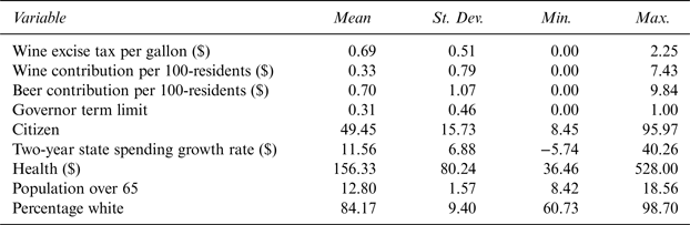
Note: Time Period: 1996–2012, N = 432 (9 years * 48 states).
The mean wine excise tax rate is $.69. There is a lot of variation among states in terms of wine excise taxes. While states like New Hampshire, Pennsylvania, Utah, and Wyoming do not have wine excise taxes,Footnote 6 Florida has the highest excise tax of $2.25. There is a huge variation between states in terms of wine contribution per 100 state residents. While Oregon has a wine contribution per 100 residents of $7.43, there are multiple states that do not have wine contributions. Beer contribution per 100 residents also varies significantly between states. While Beer in Mississippi is $9.84, there are a large number of states without any beer campaign contributions. There is notable variation among citizen ideologies between states. Kentucky is the “most conservative” state with the score of 8.45 while Vermont is the “most liberal” state with a score of 95.97. The Growth_Rate variable also varies significantly from –5.74% in Louisiana to 40.26% in Vermont and so does Health. Louisiana spends approximately $36 per person on its health expenditures while Wyoming spends a staggering $528. Utah has the least percentage of population over the age of 65 while Florida has the most. Mississippi has the least percentage of Caucasian population in the United States while Maine has the most.
Any panel study lacks effectiveness if there is no within and between variation in variables used in a study. For example, two major variables in this study, Tax and Wine varied widely within and between states in the sample. For instance, in 1996, Tax was $0.23 in Illinois, $0.45 in Idaho, $1.07 in Iowa, and $2.25 in Florida. In Illinois, it increased to $0.73 in 2000 and $1.39 in 2010. Similar variation was present for Wine as well.
Since I hypothesize that the dependent variable and the independent variables have spatial component to them, I employ the SDM for this study. For readers not familiar with spatial models, I will first explain a family of related spatial models and then the model choice, SDM. The family of related spatial models can be represented as follows:
 $$y_{it} = \rho \mathop \sum \nolimits _{\,j = 1}^N w_{ij}y_{\,jt} + \; x_{it}\beta + \theta \mathop \sum \nolimits _{\,j = 1}^N w_{ij}x_{it} + \; \mu _i + \; \lambda _t + \; u_i$$
 $$u_i = \; \delta \mathop \sum \nolimits _{\,j = 1}^N w_{ij}u_{it} + \; \varepsilon _{it}$$
where i represents cross-sectional units. For the purposes of this article, i represents U.S. states and ranges from i = 1 to N, t represents the time dimension, year, and ranges from t = 1 to N . Therefore, y it represents an observation for the dependent variable in state i in year t.
The explanatory variable, x it, is a row vector of observations with dimension (1 × K). In equation (1), β is a (1 × K) vector of parameters associated with x it variables, and is fixed and unknown. The terms μ i and λ t represent space fixed effects and time fixed effects, respectively.
The spatially-lagged dependent variable and spatially-lagged explanatory variables are represented by ρ and θ, while the spatially-lagged error term is represented by δ. The addition of these terms in association with w ij make the above model a spatial econometric model. In the model, w ij is an element of a spatial weight matrix, W. W symbolizes “neighbor-to-neighbor” relationships and has a (N × N) dimension. For example, if i and j are defined as neighbors, the w ij element is assigned a value of “1,” and “0” otherwise. In creating weight matrices, W is designed to be row-stochastic, meaning that rows of W sum to one. Hence, the term, Wy represents the weighted average of the surrounding y's. Similarly, Wx represents the weighted average of the surrounding explanatory variables, and Wu represents the surrounding error terms.
Since equation (1) characterizes a family of spatial models, restricting parameters in the equation generates various spatial econometric models. By restricting θ and δ to 0, I get spatial dependence only in the dependent variable. This type of model is called a Spatial Autoregressive Model (SAR). By setting ρ = 0 and δ = 0, I see spatial dependence only in the independent variable. Such model is named the Spatial Lag of X (SLX) model. Similarly, setting ρ = 0 and θ = 0, I see spatial dependence only in the error term; this model is named Spatial Error Model (SEM). SDM is obtained by setting δ to 0. Spatial Durbin Error Model (SDEM) is represented by equation (1). Space fixed effects (μ i) and time fixed effects (λ t) in equation (1) may be included in all models described earlier.
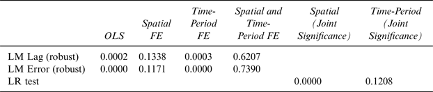
Table 2 reports Elhorst test findings for determining the presence of space- and time-fixed effects (Elhorst, Reference Elhorst, Fischer and Getis2009). The Lagrange Multiplier (LM) tests check whether there is spatial correlation in the data. The null hypothesis, H o : No spatial dependence in the dependent variable, is tested by the LM Lag test, whereas, the null hypothesis, H o : No spatial dependence in the error term, is tested by the LM Error test for each specification. Standard Likelihood Ratio (LR) tests are performed to determine the joint significance of space- and time-fixed effects (Elhorst, Reference Elhorst2014). The null hypotheses for such tests is that the presence of state fixed effects and year fixed effects are represented by:
 $$H_o\; :\; \mu _1,\mu _2,\mu _3, \ldots \mu _N = 0$$
 $$H_o\; :\; \lambda _1,\lambda _2,\lambda _3, \ldots, \; \lambda _N = 0$$
Looking at the results of Table 2, the most appropriate model is one including just the time fixed effects.
Table 2 Lagrange Multiplier (LM) and Likelihood Ratio (LR) Tests for the Presence of Spatial-and Time-Fixed Effects

FE denotes fixed effects.
Source: Author's calculations.
The next step for any spatial econometric analysis is to determine whether to choose the SAR, SEM, or SDM model. Following Elhorst (Reference Elhorst2010), I employ the standard LM tests to determine whether either the SAR or SEM model is most appropriate. The LM lag test checks whether there is spatial dependence in the dependent variable, whereas, the LM error test checks whether there is spatial dependence in the error term. Estimates of the SDM are used to generate a LR to determine whether SAR or SEM should be used instead of the SDM. In order to do this, the following hypotheses are tested:
 $$H_o\,:\,\theta = 0$$
 $$H_o\; :\; \theta + \rho \beta \; = 0$$
where θ and β are the same as in equation (1). Both tests are one-way tests. Hence, they only test the specific type spatial dependency that one is accounting for. For example, LM Lag test only accounts for spatial dependency in the dependent variable while the LM Error test only accounts for spatial dependency in the error term. The robust LM tests, however, take into account the other type of spatial dependency as well. For instance, LM Lag Robust test also takes into account spatial dependency in the error term. Likewise, the LM Error Robust test takes into account spatial dependency in the dependent variable. Both tests follow a chi-squared distribution with one degree of freedom.
Equation (4) tests the hypothesis whether SDM can be reduced to SAR. Equation (5) tests whether SDM can be reduced to SEM. SDM is the most appropriate model to use if both hypotheses are rejected. However, if H o : θ = 0 is not rejected, then SAR is the most appropriate model if the robust LM tests point towards SAR. Likewise, if H o : θ + ρβ = 0 is not rejected, SEM is the most appropriate model if the robust LM tests point towards SEM. SDM is used if one of the conditions are not met.
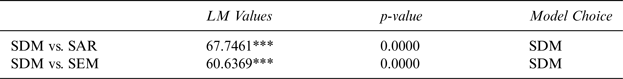
Table 3 reports the test statistics of the LM Lag and LM Error tests. As both H o : θ = 0 andH o : θ + ρβ = 0 are rejected, the most appropriate model choice is the SDM. In addition, LeSage and Pace (Reference LeSage and Pace2009) make the point that if one believes that there are spatially correlated omitted variables in the model and that these omitted variables are correlated with an explanatory variable included in the model, SDM is the most appropriate model to use. Since unseen network effects might exist between states which could be spatially related (which is captured by the error term) and can also affect, for instance, wine or beer contributions, I believe that SDM is the most appropriate model to use.Footnote 7
Table 3 Lagrange Multiplier (LM) and Likelihood Ratio (LR) Tests for the Presence of Spatial- and Time-Fixed Effects
*** denotes statistical significance at the 1% level.
Source: Author's calculations.
To fully understand the effects of the explanatory variables in the SDM, it is imperative to have an understanding of how the beta coefficient is interpreted. In SDM, unlike in a regular linear model, β does not only represent the marginal effects, meaning—an increase in β not only captures the explanatory variable changes and how it affects the dependent variable, but now captures the average direct, average indirect, and average total effects (LeSage and Pace, Reference LeSage and Pace2009), which they term effects estimates.
Since models with a spatially-lagged dependent variable have estimates that are hard to interpret, the data generating process in reduced form for such models (in this case, SDM) can be mathematically written asFootnote 8:
 $$y = \rho Wy + X\beta + WX\theta + \; \varepsilon$$
 $$y = (I_n - \; \rho W)^{ - 1}\left( {X\beta + \; WX\theta} \right) + \; \left( {I_n - \; \rho W} \right)^{ - 1}\varepsilon $$
 $$\left( {I_n - \; \rho W} \right)^{ - 1} = I_n + \rho W + \rho ^2W^2 + \cdots + \rho ^qW^{q} $$
 $$S_r\left( W \right) = \; \displaystyle{{\partial y} \over {\partial x_r}} = \; (I_n - \; \rho W)^{ - 1}\left( {\beta \;+ \; W\theta} \right)\; $$
The “r” subscript in the S r(W) represents individual explanatory variable in the X matrix.
In SDM, S r(W) is intended to capture the average direct, average indirect and, average total effects of the change in a variable on the dependent variable and can be mathematically shown as follows:
 $$Average\; Direct\; Effect:\; \displaystyle{{\partial E\left( {y_i} \right)} \over {\partial x_{ir}}} = \; S_r\left( W \right)_{ii}$$
 $$Average\; Indirect\; Effect:\; \displaystyle{{\partial E\left( {y_i} \right)} \over {\partial x_{\,jr}}} = \; S_r\left( W \right)_{ij}$$
The meaning of average direct effects can be interpreted as follows. For example, if Wine of state i is changed, how does it affect the Tax in state i? This is called i′s own effects. However, average direct effect also captures spillover effects, in which the change in Wine in state i affects Wine in its neighboring statej, which, again, “feeds back” to state i. This is called the feedback effect. The average of the diagonal elements of the S r(W) matrix captures both, own effect and the feedback effect, and is called the average direct effect.
The average indirect effect captures spillovers effects of a change in an explanatory variable in state i and how that affects observations in neighboring state j, where state i and j are not the same. This effect is captured by the average of the off-diagonal elements of the S r(W) matrix. Since the indirect effects are cumulated over all neighbors, its magnitude is usually larger than the direct effects. Finally, the average total effect is the summation of the average direct effect and the average indirect effect.
The advantage of using the SDM panel is twofold. First, it provides effect estimates that account for spatial dependence in the dependent variable, which is a much richer set of results that non-spatial panel models do not capture because they assume independence among observations. The ρ parameter captures this in this study. As data shows neighboring states changing their excise tax rates, not accounting for spatial dependence if it is present results in incorrect estimates (LeSage and Dominguez, Reference LeSage and Dominguez2012). Second, the SDM is not restricted to have the same-sign effect estimates, which the SAR model does (Elhorst, Reference Elhorst2010).
III. Empirical Results and Robustness Checks
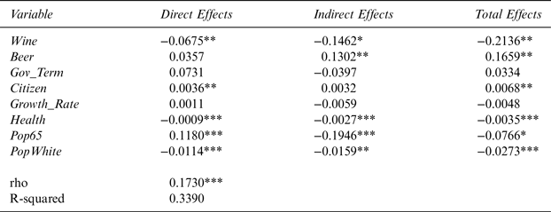
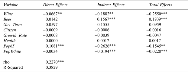
Table 4 reports the results of the effect of wine-industry campaign contributions to officials running for state offices on state wine excise tax rates. It consists of the average direct, average indirect, and average total effects estimates from the panel data SDM. The key finding is that the ρ parameter is statistically significant at the 1% level and is positive. The statistical significance of ρ establishes that state wine excise taxes are spatially correlated. The table also shows that the signs of the major variables of interest, Wine and Beer, are as expected and that Wine is statistically robust at the 5% level. In addition, six out of the eight variables used in the study are statistically significant. The results show that an increase in Wine in a state decreases Tax and has a negative average direct, indirect, and total effect.
Table 4 The Effect of Wine-Industry Campaign Contributions on Wine Excise Taxes for 48 Contiguous U.S. States Using 4-Nearest-Neighbor Matrix

Note: Dependent variable is the state wine excise tax. *,**, and *** denote statistical significance at the 10, 5, and 1% levels, respectively.
Source: Author's calculations.
The direct and total effects are statistically significant at the 5% level, whereas, the indirect effect is significant at the 10% level.
Since beer and wine can be considered as substitutes for one another, it can be hypothesized that higher amounts of campaign contributions from the beer industry in a state would earn political favors for the beer industry and possibly lead to an increase in wine excise taxes for any given amount of campaign spending. The signs for the average direct, indirect, and total effects of Beer on Tax are as expected. The effect is statistically significant at the 5% level.
Gov_Term, Citizen, Pop65, and PopWhite have total effects signs as expected. A positive Citizen total effects sign is consistent with the expectation that states leaning towards a more liberal ideology favor higher taxes on wine. Growth_Rate and Health are expected to have positive total effects estimates but have surprising negative signs.
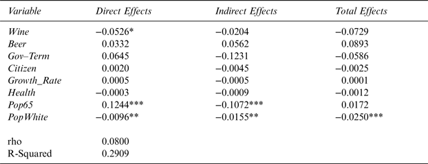
As a robustness check, I conducted spatial analysis using only 44 states (excluding the 4 control states) in the mainland United States, reported in Table 5. The main finding of this robustness check is that ρ parameter possesses the same sign as ρ in Table 4, and is also significant at the 1% level. This finding is especially important because it establishes an existence of a spatial correlation, even while controlling for “control” states. The signs of the major variables of interests are the same as in Table 4. The statistical significance of the Wine direct effect stays the same. However, the statistical significance of Wine indirect effect increases and is now significant at the 5% level. Wine total effects is statistically robust at the 1% level. Citizen loses significance and so does Health. The sign for Citizen is not as expected. However, it is so for Health.
Table 5 The Effect of Wine-Industry Campaign Contributions on Wine Excise Taxes for 44 Contiguous U.S. States Using 4-Nearest-Neighbor Matrix
Note: Dependent variable is the state wine excise tax. *,**, and *** denote statistical significance at the 10, 5, and 1% levels, respectively.
Source: Author's calculations.
Additionally, I also conducted a spatial analysis using 5-nearest-neighbor weight matrix. I hypothesize ρ to lose spatial significance when using a 5-nearest-neighbor weight matrix. This assumption is reasonable because the further out states are from a given state, the less impact they would have on that state. This result is reported in Table 6.
Table 6 The Effect of Wine-Industry Campaign Contributions on Wine Excise Taxes for 48 Contiguous U.S. States Using 5-Nearest-Neighbor Matrix

Note: Dependent variable is the state wine excise tax. *,**, and *** denote statistical significance at the 10, 5, and 1% levels, respectively.
Source: Author's calculations.
The results show that the ρ parameter indeed loses significance. However, Wine and Beer still hold expected signs but are not statistically robust. The signs for Health and PopWhite are the same as before. However, Gov_Term possesses a contradictory negative sign. All variables lose significance in this specification except for PopWhite.
IV. Conclusion
Given the growing importance of the wine industry for the United States, increases in campaign contributions from the wine industry to officials running for state offices, along with theoretical and empirical evidence that shows that tax rates are interdependent, I hypothesized that the wine-industry special interest influences state wine excise taxes across space. I find that there is robust statistical evidence that wine excise taxes exhibit spatial dependence, which is the key finding of this study. I find that, on average, the increases in campaign contributions from the wine industry in a state results in a decrease in wine excise taxes in the given state and its neighboring states.
There are two contributions of this study. First, it is the first study to look at the effects of campaign contributions of the alcohol industry, specifically, the wine industry on state wine excise taxes. Previously, for instance, special interest group literature have looked at the tobacco industry. Second, it is also the first study to look at the wine industry using a spatial econometric model. One of the distinguishing and important ability of spatial econometric models is that they can empirically test for the presence of spatial dependency and quantify spillover effects. In the context of this article, the use of SDM showed the reader that there is robust statistical evidence of spatial dependency in wine excise taxes among states. Not accounting for these indirect effects when they are clearly present could provide biased estimates. Therefore, one application of spatial models is that given its ability to test for spatial dependence, policymakers and economists should account for spillover effects while making informed policy proposals.
Moving forward, future projects could look at establishing a causal relationship between wine production and wine excise taxes across time once production data for all 50 states become available. In addition, future research could look at the political economy of campaign contributions. One example could be to look at the channels through where these effects take place. For instance, looking at which state offices most likely influence decisions could be a starting point.