NOMENCLATURE
- a
Constant of intermolecular forces
- b
Constant of molecular size
- f 1, f 2
Nonlinear equations
- x
Abscissa of the nozzle section
- y
Radius of the nozzle section
- A
Section area
- C F
Thrust coefficient
- C Mass
Non-dimensional nozzle mass
- C P
Specific heat to constant pressure
- C T
Specific heat at constant temperature
- C −
Function for first compatibility equation
- C +
Function for second compatibility equation
- D −
Function for first characteristics equation
- D +
Function for second characteristics equation
- E (T)
First function for energy equation
- E (ρ)
Second function for energy equation
- G
Value for MOC model
- L
Length of the nozzle
- M
Mach number
- N
Number of points on the wall
- P
Pressure
- R
Gas constant
- S V
Sound velocity
- T
Temperature
- V
Flow velocity
- Δ
Step on the uniform Mach line
- Δθ
Step for ξ from the expansion centre
- α
molecular vibration energy constant
- γ
Specific heats ratio
- δ
δ = 0 for 2D and δ = 1 for axisymmetric
- ε
Tolerance of calculation (desired precision)
- η
Right-running characteristic
- θ
Flow angle deviation
- μ
Mach angle
- ν
Prandtl Meyer function
- ν (T)
First part for Prandtl Meyer function
- ν (ρ)
Second part for Prandtl Meyer function
- ξ −
Left-running characteristic
- ρ
Density
Abbreviation
- ABE
Transition zone
- BES
Uniform triangular zone
- CFD
Computational fluid dynamics
- HT
High Temperature model
- MLN
Minimum Length Nozzle
- MOC
Method of Characteristics
- NPR
Nozzle Pressure Ratio
- OA
Sonic line
- OAB
Kernel zone
- PG
Perfect Gas model
- PM
Prandtl Meyer function
- RG
Real Gas model
Subscripts
- j
Point
- A
Throat of the nozzle
- E
Exit section
- K
For numerical iteration process
- 0
Stagnation condition (combustion chamber)
- 1
Point 1
- 2
Point 2
- 3
Point 3
- 13
Average value between points 1 and 3
- 23
Average value between points 2 and 3
- *
Critical condition
1.0 INTRODUCTION
In aeronautics and aerospace engineering construction, the supersonic nozzle, in particular the Minimum Length Nozzle (MLN), is of interest for propelling aerospace machines and defence propulsion technology. The design of the supersonic nozzles is an important phase before moving to construction and realisation. The axisymmetric geometry is preferred in aerospace construction, as well as 2D geometry for wind tunnel test construction. The nozzle giving a uniform and parallel flow to the exit section is very interesting for propulsion with maximum thrust and other considerations for wind tunnels(Reference Peterson and Hill1–Reference Emanuel and Argrow3). The design necessarily depends on the conditions of the combustion chamber. The latter makes a chemical reaction of the gases selected under T 0 and P 0 conditions giving chemical compositions of the gases with specific heat ratio at the end of combustion(Reference Peterson and Hill1–Reference Emanuel and Argrow3). The physical behaviour of gas in the diverging supersonic part essentially depends on these two stagnation parameters and other data like specific heat at constant pressure and the specific heat ratio γ. Then, the shape of the nozzle depends again on the two parameters. Thus, the design calculation of the nozzle is usually made based on a non-viscous flow. When the nozzle enters the flow, the fluid is actually viscous and will give birth to a boundary layer.
The second problem of the birth of the side loads is generally related to the vibration of the nozzle in the presence of the real flow in the nozzle and the increase of the static pressure when the nozzle enters the regime of the non-adaptation and increase of the nozzle pressure ratio (NPR) of the nozzle.
During the flow, one cannot change the shape of the nozzle to leave the nozzle always in adaptation regime to avoid the side loads. Also, one cannot force the fluid to be non-viscous to avoid the boundary layer and, therefore, the separation of the flow from the wall of the nozzle. For this reason, the return to regime of the non-adaptation and the side loads are phenomena always to be observed in the supersonic nozzle(Reference Ostlund, Damgaad and Frey4–Reference Ralf and Chloe7).
When the nozzle is adapted, the expansion of the flow is complete and gives the desired exit Mach number in the calculation. When the nozzle enters into flow in reality and when the nozzle enters the non-adaptation regime given the increase or the variation of the NPR number of the nozzle, the expansion will not be complete and there will inevitably be a remarkable reduction in the exit Mach number, resulting in an increase in pressure. In this case, the flow finds a reduced space in the nozzle to make its expansion, and due to the flow separation that will decrease the Mach number distribution, it will consequently have an increase in pressure (which is a bad thing at the nozzle and flow). This pressure increase in nozzle locations and the instability of the flow will generate a nozzle vibration justified by the generation of side loads having a magnitude that varies with the rate of increase of NPR and the instability of the nozzle. It can be said that these phenomena do not exist when the nozzle is adapted.
Since the shape of the nozzle is unchangeable during the flow and since there is an increase in the NPR of the nozzle, the behaviour of the flow to be forced causes these phenomena in a fixed space limited by the wall of the nozzle, meaning that the shape of the nozzle is also responsible for these phenomena. Then, it is estimated that the shape of the nozzle, which cannot be changed during flow in all phases of flight, and the actual non-viscous fluid behaviour cause the birth of these two phenomena.
In these cases, the separation of the flow from the wall and the birth of the side load are observed inside the nozzle. The size of the side load depends on NPR and on the size of the nozzle, which in some cases can cause an exposure of the nozzle. To avoid this problem, it is necessary to respect the real behaviour of the gas inside the nozzle during the flow. Then, the assumptions made for the design calculation are very interesting and will be discussed positively or negatively after a wind tunnel test.
In Refs Reference Peterson and Hill1–Reference Emanuel and Argrow3, the authors have studied the design of the supersonic nozzle based on the calorically and thermally perfect gas (PG). These studies are done without considering the effect of T 0 and P 0 of the combustion chamber. Wind tunnel tests show that the results obtained by the PG model are accepted when M E<2.00 and T 0<240 K (if air is used) and no information on the effect of the P 0 value. This is a very limited area and does not reflect the current need for aerospace construction.
In Refs Reference Abada, Zebbiche and Abdallah El-Hirtsi8–Reference Zebbiche and Youbi10, the authors improved the search by taking into account the effect of T 0 under the threshold of the molecules’ dissociation, without taking into account the value of P 0, and consequently, they have somewhat widened the real scope of the application. These studies are applied if ME<5.00 and T 0<3,550K (if air is used) but no indication of the value of P 0. To allow the design to be made according to the hypotheses of these references, the authors have developed a new approach to the thermodynamic parameters(Reference Zebbiche and Youbi11) as well as for the Prandtl Meyer (PM) function(Reference Zebbiche12,Reference Zebbiche and Boun-Jad13) .
In Ref. Reference Boun-Jad, Zebbiche and Allali14, the authors studied the effect of the propulsion gas on the shape of MLN at high temperature (HT) assumption without taking into account the value of P 0. The field of application remains always rather limited according to the reality of the current need. In the same context of the research, a new application of the gas effect on the PM is presented in Ref. Reference Boun-Jad, Zebbiche and Allali15.
The aim of this work is to develop a computational model and numerical program to design the supersonic nozzles giving a uniform and parallel flow to the exit section by a new model of generalised Method of Characteristics (MOC) considering the values of P 0 and T 0 of the combustion chamber. The application will be made for 2D and axisymmetric MLN, given its practical interest in the aerospace construction and need to bring the maximum possible towards the actual behaviour of the flow when P 0 will be high. To develop this model of MOC, the vision is made on the consideration of the principle of real gas (RG), given the size of the molecules and the heat imperfection of gas effect with P 0 effect. The Berthelot state equation is used in this case, and the application is made for air. The comparison is made with the PG and HT models given their practical importance in the international community. To reduce the size of flow separation and the side loads intensity for our needs, it is recommended in a few ways to size the nozzle with an exit Mach number enough and slightly higher than that desired for the real flow to increase a little the size of the nozzle. For side loads, it is recommended to use our present study by determining the contours of the supersonic nozzle as a function of the stagnation pressure P 0 of the combustion chamber, since the stagnation pressure P 0 and the ambient pressure Pa are those that are responsible for NPR number of the nozzle (NPR= P 0/P a).
2.0 MATHEMATICAL FORMULATION
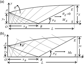
Figure 1 shows the 2D and axisymmetric MLN with the different flow regions to have a uniform and parallel flow at the exit section. The Kernel OAB area, the transition ABE area and the uniform triangular BES area are noted. The Kernel region is a non-simple area, where the characteristics are curved for both geometries. The transition region is a non-simple zone for the axisymmetric case and of a simple type for the 2D case. In the latter, the rising characteristics are straight lines. In the uniform BES area, the two characteristics lines are straight lines. It should be noted that in international regulations the two lines of upward and downward characteristics are presented in the non-simple zone, only the straight lines in the simple zone are shown and in the uniform zone nothing is presented. This is the case for both Figures 1(a) and 1(b).

Figure 1. Flow field inside the supersonic 2D and axisymmetric MLN giving a uniform and parallel flow at the exit section. (a) 2D geometry. (b) Axisymmetric geometry.
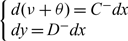
The compatibilities and characteristics equations valid on ξ and η of Figure 2 in differential form(Reference Anderson16) can be written by:
 $$\begin{equation}
\left\{\begin{array}{l} {d(\nu +\theta ) = C^{-} dx} \\ {dy = D^{-} dx} \end{array}\right.
\end{equation}
$$
$$\begin{equation}
\left\{\begin{array}{l} {d(\nu +\theta ) = C^{-} dx} \\ {dy = D^{-} dx} \end{array}\right.
\end{equation}
$$
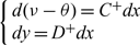 $$\begin{equation}
\left\{\begin{array}{l} {d(\nu -\theta ) = C^{+} dx} \\ {dy = D^{+} dx} \end{array}\right.
\end{equation}
$$
$$\begin{equation}
\left\{\begin{array}{l} {d(\nu -\theta ) = C^{+} dx} \\ {dy = D^{+} dx} \end{array}\right.
\end{equation}
$$
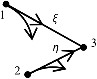
Figure 2. Downward and upward Mach lines.
In thermodynamics, all state parameters can be defined by two state variables(Reference Thompson17–Reference Salhi, Zebbiche and Mehalem21), chosen by T and ρ in our study.
From the differential form(Reference Van Wylen18–Reference Salhi and Zebbiche20,Reference Raltson and Rabinowitz22) , the Bernoulli equation can be written by:
 $$\begin{equation}
E^{(\rho )} d\rho = E^{(T)} dT
\end{equation}
$$
$$\begin{equation}
E^{(\rho )} d\rho = E^{(T)} dT
\end{equation}
$$
 $$\begin{equation}
E^{(T)} = \frac{C_{P} (T,\rho )}{S_{V}^{2} (T,\rho )} \; ,\; E^{(\rho )} = \frac{1}{\rho } -\frac{C_{T} (T,\rho )}{S_{V}^{2} (T,\rho )}
\end{equation}
$$
$$\begin{equation}
E^{(T)} = \frac{C_{P} (T,\rho )}{S_{V}^{2} (T,\rho )} \; ,\; E^{(\rho )} = \frac{1}{\rho } -\frac{C_{T} (T,\rho )}{S_{V}^{2} (T,\rho )}
\end{equation}
$$
In differential form, the PM is given by Refs Reference Salhi, Zebbiche and Roudane23 and Reference Salhi, Zebbiche and Mehalem24
 $$\begin{equation}
d\nu =-\nu ^{(T)} dT-\nu ^{(\rho )} d\rho
\end{equation}
$$
$$\begin{equation}
d\nu =-\nu ^{(T)} dT-\nu ^{(\rho )} d\rho
\end{equation}
$$
With
 $$\begin{equation}
\nu ^{(T)} = \frac{\sqrt{M^{2} (T,\rho )-1} }{V^{2} (T,\rho )} C_{P} (T,\rho )
\end{equation}
$$
$$\begin{equation}
\nu ^{(T)} = \frac{\sqrt{M^{2} (T,\rho )-1} }{V^{2} (T,\rho )} C_{P} (T,\rho )
\end{equation}
$$
 $$\begin{equation}
\nu ^{(\rho )} = \frac{\sqrt{M^{2} (T,\rho )-1} }{V^{2} (T,\rho )} C_{T} (T,\rho )
\end{equation}
$$
$$\begin{equation}
\nu ^{(\rho )} = \frac{\sqrt{M^{2} (T,\rho )-1} }{V^{2} (T,\rho )} C_{T} (T,\rho )
\end{equation}
$$
and
 $$\begin{equation}
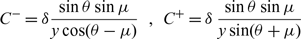
C^{-} = \delta \frac{\sin \theta \sin \mu }{y \cos (\theta -\mu )} \; \; \; ,\; \; C^{+} = \delta \; \frac{\sin \theta \sin \mu }{y\sin(\theta +\mu )}
\end{equation}
$$
$$\begin{equation}
C^{-} = \delta \frac{\sin \theta \sin \mu }{y \cos (\theta -\mu )} \; \; \; ,\; \; C^{+} = \delta \; \frac{\sin \theta \sin \mu }{y\sin(\theta +\mu )}
\end{equation}
$$
 $$\begin{equation}
D^{-} = \tan (\theta -\mu )\; \; ,\; \; \; D^{+} = \tan (\theta +\mu )
\end{equation}
$$
$$\begin{equation}
D^{-} = \tan (\theta -\mu )\; \; ,\; \; \; D^{+} = \tan (\theta +\mu )
\end{equation}
$$
 $$\begin{equation}
M= \frac{V(T,\rho )}{S_{V} (T,\rho )}
\end{equation}
$$
$$\begin{equation}
M= \frac{V(T,\rho )}{S_{V} (T,\rho )}
\end{equation}
$$
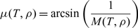 $$\begin{equation}
\mu (T,\rho ) = \arcsin \left(\frac{1}{M(T,\rho )} \right)
\end{equation}
$$
$$\begin{equation}
\mu (T,\rho ) = \arcsin \left(\frac{1}{M(T,\rho )} \right)
\end{equation}
$$
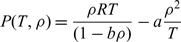
The expressions of V(T, ρ), S V(T, ρ), C T(T, ρ) and C P(T, ρ) are presented in Refs Reference Salhi, Zebbiche and Mehalem21 and Reference Nag25. The pressure can be calculated by the following Berthelot state equation(Reference Van Wylen18–Reference Salhi, Zebbiche and Mehalem21,Reference Salhi, Zebbiche and Mehalem24,Reference Nag25) :
 $$\begin{equation}
P(T,\rho ) = \frac{\rho R T}{(1-b\rho )} -a \frac{\rho ^{2} }{T}
\end{equation}
$$
$$\begin{equation}
P(T,\rho ) = \frac{\rho R T}{(1-b\rho )} -a \frac{\rho ^{2} }{T}
\end{equation}
$$
For PG and HT models, all the physical parameters can be determined according to one variable, which can be the chosen Mach number for the PG model and the temperature for the HT model for numerical reason. But for our presented RG model, all the thermodynamic parameters depend on two state variables, which are T and ρ.
For air, we have γ PG = 1.402, R = 287.1029 J/(kg K), a = 117.2666 Pa m6, b = 1.07334 m3 and α = 3, 056.0K(18–22,25).
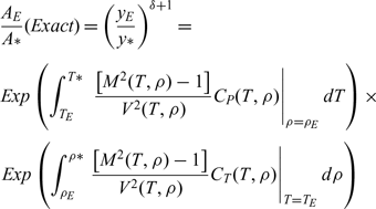
As the flow is 1D at the throat and exit sections, Equation (13) remains valid for the validation of the numerically obtained results(Reference Salhi, Zebbiche and Mehalem21,Reference Nag25) .
 $$\matrix{
{{\rm{ }}{{{A_E}} \over A}(Exact) = {{\left( {{{{y_E}} \over y}} \right)}^{\delta + 1}} = } \cr
{Exp\left( {\int_{{T_E}}^{T*} {{{\left. {\;{{\left[ {{M^2}(T,\rho ) - 1} \right]} \over {{V^2}(T,\rho )}}{C_P}(T,\rho )} \right|}_{\rho = {\rho _E}}}} dT} \right) \times } \cr
{Exp\left( {\int_{{\rho _E}}^{\rho *} {{{\left. {{{\left[ {{M^2}(T,\rho ) - 1} \right]} \over {{V^2}(T,\rho )}}{C_T}(T,\rho )} \right|}_{T = {T_E}}}} d\rho } \right)} \cr
} {\rm{ }}\qquad \qquad \qquad \qquad $$
$$\matrix{
{{\rm{ }}{{{A_E}} \over A}(Exact) = {{\left( {{{{y_E}} \over y}} \right)}^{\delta + 1}} = } \cr
{Exp\left( {\int_{{T_E}}^{T*} {{{\left. {\;{{\left[ {{M^2}(T,\rho ) - 1} \right]} \over {{V^2}(T,\rho )}}{C_P}(T,\rho )} \right|}_{\rho = {\rho _E}}}} dT} \right) \times } \cr
{Exp\left( {\int_{{\rho _E}}^{\rho *} {{{\left. {{{\left[ {{M^2}(T,\rho ) - 1} \right]} \over {{V^2}(T,\rho )}}{C_T}(T,\rho )} \right|}_{T = {T_E}}}} d\rho } \right)} \cr
} {\rm{ }}\qquad \qquad \qquad \qquad $$
3.0 CALCULATION PROCEDURE FOR INTERNAL POINTS
The problem is to calculate (T, ρ, θ, x, y) at point 3 of Figure 2 by solving Equations (1–3). The parameters in each point are related to the upstream points 1 and 2. The values of M 3 and P 3 are determined by the relations (10) and (12). The ratios T/T 0, ρ/ρ 0 and P/P 0 can then be determined.
After integration of Equations (1–3), five nonlinear algebraic equations are obtained. Their resolution is done by the predictor corrector algorithm of the finite difference method(Reference Raltson and Rabinowitz22). Then, the thermo-physical properties at point 3 can be determined by the following equations:
 $$\begin{equation}
x_{3} =\frac{G_{2} -G_{1} }{D_{13}^{-} }
\end{equation}
$$
$$\begin{equation}
x_{3} =\frac{G_{2} -G_{1} }{D_{13}^{-} }
\end{equation}
$$
 $$\begin{equation}
y_{3} = G_{1} +D_{13}^{-} x_{3}
\end{equation}
$$
$$\begin{equation}
y_{3} = G_{1} +D_{13}^{-} x_{3}
\end{equation}
$$
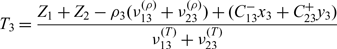 $$\begin{equation}
T_{3} = \frac{Z_{1} +Z_{2} -\rho _{3} (\nu _{13}^{(\rho )} +\nu _{23}^{(\rho )} )+(C_{13}^{-} x_{3} +C_{23}^{+} y_{3} )}{\nu _{13}^{(T)} +\nu _{23}^{(T)} }
\end{equation}
$$
$$\begin{equation}
T_{3} = \frac{Z_{1} +Z_{2} -\rho _{3} (\nu _{13}^{(\rho )} +\nu _{23}^{(\rho )} )+(C_{13}^{-} x_{3} +C_{23}^{+} y_{3} )}{\nu _{13}^{(T)} +\nu _{23}^{(T)} }
\end{equation}
$$
 $$\begin{equation}
\theta _{3} ={ Z}_{1} -\nu _{13}^{(\rho )} \rho _{3} +C_{13}^{-} x_{3} -\nu _{13}^{(T)} T_{3}
\end{equation}
$$
$$\begin{equation}
\theta _{3} ={ Z}_{1} -\nu _{13}^{(\rho )} \rho _{3} +C_{13}^{-} x_{3} -\nu _{13}^{(T)} T_{3}
\end{equation}
$$
 $$\begin{equation}
\rho _{3} =\rho _{1} +\frac{E_{13}^{(T)} }{E_{13}^{(\rho )} } (T_{3} -T_{1} )
\end{equation}
$$
$$\begin{equation}
\rho _{3} =\rho _{1} +\frac{E_{13}^{(T)} }{E_{13}^{(\rho )} } (T_{3} -T_{1} )
\end{equation}
$$
Where
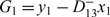 $$\begin{equation}
G_{1} = y_{1} -D_{13}^{-} x_{1}
\end{equation}
$$
$$\begin{equation}
G_{1} = y_{1} -D_{13}^{-} x_{1}
\end{equation}
$$
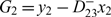 $$\begin{equation}
G_{2} = y_{2} -D_{23}^{-} x_{2}
\end{equation}
$$
$$\begin{equation}
G_{2} = y_{2} -D_{23}^{-} x_{2}
\end{equation}
$$
 $$\begin{equation}
Z_{1} = \theta _{1} +\nu _{13}^{(T)} T_{1} +\nu _{13}^{(\rho )} \rho _{1} -C_{13}^{-} x_{1}
\end{equation}
$$
$$\begin{equation}
Z_{1} = \theta _{1} +\nu _{13}^{(T)} T_{1} +\nu _{13}^{(\rho )} \rho _{1} -C_{13}^{-} x_{1}
\end{equation}
$$
 $$\begin{equation}
Z_{2} ={ -}\theta _{2} +\nu _{23}^{(T)} T_{2} +\nu _{23}^{(\rho )} \rho _{2} -C_{23}^{-} y_{2}
\end{equation}
$$
$$\begin{equation}
Z_{2} ={ -}\theta _{2} +\nu _{23}^{(T)} T_{2} +\nu _{23}^{(\rho )} \rho _{2} -C_{23}^{-} y_{2}
\end{equation}
$$
The values of  ${\nu _{13}^{(T)} }$,
  ${\nu _{13}^{(\rho )} }$,
  ${C_{{13}}^{-} }$,
  ${E_{13}^{(T)} }$,
  ${E_{13}^{(\rho )} }$ and
  ${D_{13}^{-} }$ can be determined respectively by the relations (6), (7), (8) and (4) by replacing T= T 13 and ρ = ρ 13, and the values of
  ${\nu _{23}^{(T)} }$,
 ${\nu _{23}^{(\rho )} }$,
  ${C_{{23}}^{+} }$,
  ${E_{23}^{(\rho )} }$,
  ${E_{23}^{(T)} }$ and
  ${D_{23}^{+} }$ are determined by replacing T = T 23 and ρ = ρ 23. The values of x 13, y 13, T 13, θ 13, ρ 13 and x 23, y 23, T 23, θ 23 et ρ 23 are taken as average values by:
 $$\begin{equation}
T_{13} =(T_{1} +T_{3}^{0} )/2{ \; \; ,\; \; \; }T_{23} =(T_{2} +T_{3}^{0} )/2
\end{equation}
$$
$$\begin{equation}
T_{13} =(T_{1} +T_{3}^{0} )/2{ \; \; ,\; \; \; }T_{23} =(T_{2} +T_{3}^{0} )/2
\end{equation}
$$
 $$\begin{equation}
\theta _{13} =(\theta _{1} +\theta _{3}^{0} )/2{ \; \; ,\; \; \; }\theta _{23} =(\theta _{2} +\theta _{3}^{0} )/2
\end{equation}
$$
$$\begin{equation}
\theta _{13} =(\theta _{1} +\theta _{3}^{0} )/2{ \; \; ,\; \; \; }\theta _{23} =(\theta _{2} +\theta _{3}^{0} )/2
\end{equation}
$$
 $$\begin{equation}
x_{13} =(x_{1} +x_{3}^{0} )/2{ \; \; ,\; \; \; }x_{23} =(x_{2} +x_{3}^{0} )/2
\end{equation}
$$
$$\begin{equation}
x_{13} =(x_{1} +x_{3}^{0} )/2{ \; \; ,\; \; \; }x_{23} =(x_{2} +x_{3}^{0} )/2
\end{equation}
$$
 $$\begin{equation}
y_{13} =(y_{1} +y_{3}^{0} )/2{ \; \; ,\; \; \; }y_{23} =(y_{2} +y_{3}^{0} )/2
\end{equation}
$$
$$\begin{equation}
y_{13} =(y_{1} +y_{3}^{0} )/2{ \; \; ,\; \; \; }y_{23} =(y_{2} +y_{3}^{0} )/2
\end{equation}
$$
 $$\begin{equation}
\rho _{13} =(\rho _{1} +\rho _{3}^{0} )/2{ \; \; ,\; \; \; }\rho _{23} =(\rho _{2} +\rho _{3}^{0} )/2
\end{equation}
$$
$$\begin{equation}
\rho _{13} =(\rho _{1} +\rho _{3}^{0} )/2{ \; \; ,\; \; \; }\rho _{23} =(\rho _{2} +\rho _{3}^{0} )/2
\end{equation}
$$
The predicted values at (K = 0) of x 3, y 3, T 3, θ 3 et ρ 3 are chosen by 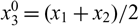 $x_{3}^{0}=(x_{1}+x_{2})/2$,
 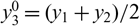 $y_{3}^{0}=(y_{1}+y_{2})/2$,
 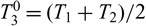 $$$T_{3}^{0}=(T_{1}+T_{2})/2$,
 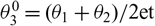 $\theta_{3}^{0}=(\theta_{1}+\theta_{2})/2$,
 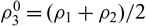 $\rho_{3}^{0}=(\rho_{1}+\rho_{2})/2$.
The corrector algorithm will be repeated until satisfying the following condition:
 $$\begin{equation}
Max \left[\begin{array}{l} { \left| x_{3}^{\:K+1} -x_{3}^{\:K} \right| , \left| y_{3}^{\:K+1} -y_{3}^{\:K} \right| , \left| T_{3}^{K+1} -T_{3}^{K} \right| ,} \\[3pt] { \left| \theta _{3}^{K+1} -\theta _{3}^{K} \right| , \left| \rho _{3}^{K+1} -\rho _{3}^{K} \right|} \end{array}\right] < \varepsilon
\end{equation}
$$
$$\begin{equation}
Max \left[\begin{array}{l} { \left| x_{3}^{\:K+1} -x_{3}^{\:K} \right| , \left| y_{3}^{\:K+1} -y_{3}^{\:K} \right| , \left| T_{3}^{K+1} -T_{3}^{K} \right| ,} \\[3pt] { \left| \theta _{3}^{K+1} -\theta _{3}^{K} \right| , \left| \rho _{3}^{K+1} -\rho _{3}^{K} \right|} \end{array}\right] < \varepsilon
\end{equation}
$$
For our RG model, the Euler corrector algorithm contains five algebraic Equations (14–18) to determine x 3, y 3, T 3, θ 3 and ρ 3. The values of M 3 and P 3 are determined analytically. Whereas for the HT model(Reference Zebbiche9), the Euler corrector algorithm contains four equations to determine x 3, y 3, T 3 and θ 3. In this case, M 3, ρ 3 and P 3 are determined analytically, and for the PG model(Reference Emanuel and Argrow3), the Euler corrector algorithm always contains four equations to determine, in this case, x 3, y 3, M 3 and θ 3. Where T 3, ρ 3 and P 3 are determined analytically.
If point 3 of Figure 2 is on the axis of symmetry, in this case, we have y 3 = 0.0 and θ 3 = 0.0. A single descending characteristic line joining points 1 and 3 is used to determine the remaining properties at point 3. Relationships (16) and (14) are no longer valid and will be replaced by the following equations. Equation (18) is still valid.
 $$\begin{equation}
T_{3} = T_{1} +\frac{C_{13}^{-} (x_{3} -x_{1} )+\theta _{1} -\nu _{13}^{(\rho )} (\rho _{3} -\rho _{1} )}{\nu _{13}^{(T)} }
\end{equation}
$$
$$\begin{equation}
T_{3} = T_{1} +\frac{C_{13}^{-} (x_{3} -x_{1} )+\theta _{1} -\nu _{13}^{(\rho )} (\rho _{3} -\rho _{1} )}{\nu _{13}^{(T)} }
\end{equation}
$$
 $$\begin{equation}
x_{3} ={ x}_{1} -\frac{y_{1} }{D_{13}^{-} }
\end{equation}
$$
$$\begin{equation}
x_{3} ={ x}_{1} -\frac{y_{1} }{D_{13}^{-} }
\end{equation}
$$
The third type of point is the point of discontinuity at the expansion centre A of Figure 1. At this point, there is a sudden increase of all the thermo-physical parameters. This discontinuity gives infinity of Mach line, which will be from point A and reflected on the axis of symmetry. In each deviation, the PM takes the following value:
 $$\begin{equation}
\nu _{j} =\theta _{j} =(j-1) \Delta \theta
\end{equation}
$$
$$\begin{equation}
\nu _{j} =\theta _{j} =(j-1) \Delta \theta
\end{equation}
$$
The problem consists in determining T j, ρ j, M j and P j corresponding to this deviation number j. Since the function ν depends on two variables, T and ρ, we must solve the following two nonlinear algebraic equations simultaneously to obtain T j and ρ j. So:
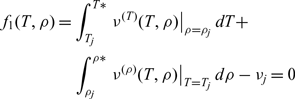 $$\begin{equation} \nonumber
{f_{1} (T, \rho )=\int _{T_{j} }^{T{*} }\left. \nu ^{(T)} (T, \rho )\right|_{\rho =\rho _{j} } dT +}
\qquad\quad\qquad\qquad{\int _{\rho _{j} }^{\rho {*} }\left. \nu ^{(\rho )} (T,\rho )\right|_{T=T_{j} } d\rho -\nu _{j} =0}
\end{equation}
$$
$$\begin{equation} \nonumber
{f_{1} (T, \rho )=\int _{T_{j} }^{T{*} }\left. \nu ^{(T)} (T, \rho )\right|_{\rho =\rho _{j} } dT +}
\qquad\quad\qquad\qquad{\int _{\rho _{j} }^{\rho {*} }\left. \nu ^{(\rho )} (T,\rho )\right|_{T=T_{j} } d\rho -\nu _{j} =0}
\end{equation}
$$
 $$\begin{equation} \nonumber
{f_{2} (T, \rho )=\int _{T_{j} }^{T{*} }\left. E^{(T)} (T, \rho )\right|_{\rho =\rho _{j} } dT- }
{\qquad\qquad\qquad\int _{\rho _{j} }^{\rho {*} }\left. E^{(\rho )} (T,\rho )\right|_{T=T_{j} } d\rho =0}
\end{equation}
$$
$$\begin{equation} \nonumber
{f_{2} (T, \rho )=\int _{T_{j} }^{T{*} }\left. E^{(T)} (T, \rho )\right|_{\rho =\rho _{j} } dT- }
{\qquad\qquad\qquad\int _{\rho _{j} }^{\rho {*} }\left. E^{(\rho )} (T,\rho )\right|_{T=T_{j} } d\rho =0}
\end{equation}
$$
The integrals in Equations (32) and (33) are evaluated by the Gauss Legendre formulae of order 20(26) to make fast computation with high precision.
The numerical techniques used to solve a system of nonlinear equations(26) are based on the Jacobean computation, which is formulated from the derivative of f 1 and f 2. The numerical tests using these methods demonstrate that the determinant of this Jacobean computation (denominator of our computation of f 1 and f 2) takes a null value during the computation, whatever the chosen of the initial vector, which immediately interrupts the calculation. For this reason and to find a solution to our problem, we have developed a fast and robust technique. It converges towards the desired solution without failure.
The flow properties must be calculated in all the points according to the mesh of Figure 1. Then, the critical section ratio corresponding to the chosen discretisation will be given by:
 $${{{A_E}} \over {A * }}(computed) = {\left( {{{{y_N}} \over {y * }}} \right)^{\delta + 1}}$$
Once the convergence is reached, the design parameters L, C Mass, C F and all the thermodynamics parameters converge towards the desired physical solution.
For the PG model(Reference Peterson and Hill1–Reference Emanuel and Argrow3), the design data are M E and γ of gas. For the HT model(Reference Abada, Zebbiche and Abdallah El-Hirtsi8–Reference Zebbiche and Youbi10,Reference Boun-Jad, Zebbiche and Allali14) , the design data are M E, T 0 and C P(T) of gas. While for our RG model, the design data are extended to M E, T 0, P 0 and C P(T, ρ) of gas. Then we can consider that the PG(Reference Emanuel and Argrow3) and HT(Reference Abada, Zebbiche and Abdallah El-Hirtsi8–Reference Zebbiche and Youbi10) models are special cases of our presented RG model. In other words, our RG model of MOC is a generalization of the PG and HT models. The model PG can be obtained from our model RG when we take a = b = α = 0, and the HT model can be determined from the RG model when a = b = 0. For the PG and HT models, the Berthelot state equation of real gas becomes the state equation of perfect gas (P = ρRT).
4.0 MASS OF THE NOZZLE
For N points found on the wall, the mass in non-dimensional form for 2D and axisymmetric geometry can be obtained respectively by:
 $$\begin{equation}
C_{Mass} =2\sum _{j=1}^{N-1}\; \sqrt{\left(\frac{x_{j+1} }{y{*} } -\frac{x_{j} }{y{*} } \right)^{2} +\left(\frac{y_{j+1} }{y{*} } -\frac{y_{j} }{y{*} } \right)^{2} }
\end{equation}
$$
$$\begin{equation}
C_{Mass} =2\sum _{j=1}^{N-1}\; \sqrt{\left(\frac{x_{j+1} }{y{*} } -\frac{x_{j} }{y{*} } \right)^{2} +\left(\frac{y_{j+1} }{y{*} } -\frac{y_{j} }{y{*} } \right)^{2} }
\end{equation}
$$
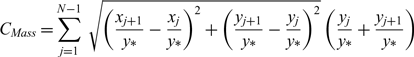 $$\begin{equation}
C_{Mass} =\sum _{j=1}^{N-1}\; \sqrt{\left(\frac{x_{j+1} }{y{*} } -\frac{x_{j} }{y{*} } \right)^{2} +\left(\frac{y_{j+1} }{y{*} } -\frac{y_{j} }{y{*} } \right)^{2} } \left(\frac{y_{j} }{y{*} } +\frac{y_{j+1} }{y{*} } \right)
\end{equation}
$$
$$\begin{equation}
C_{Mass} =\sum _{j=1}^{N-1}\; \sqrt{\left(\frac{x_{j+1} }{y{*} } -\frac{x_{j} }{y{*} } \right)^{2} +\left(\frac{y_{j+1} }{y{*} } -\frac{y_{j} }{y{*} } \right)^{2} } \left(\frac{y_{j} }{y{*} } +\frac{y_{j+1} }{y{*} } \right)
\end{equation}
$$
5.0 THRUST OF THE NOZZLE
The axial pressure force exerted on the nozzle’s wall by 2D and axisymmetric geometry, respectively, is given in non-dimensional form by:
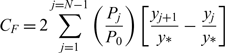 $$\begin{equation}
C_{F} =2\sum _{j=1}^{j=N-1} \left(\frac{P_{j} }{P_{0} } \right) \left[\frac{y_{j+1} }{y{*} } -\frac{y_{j} }{y{*} } \right]\;
\end{equation}
$$
$$\begin{equation}
C_{F} =2\sum _{j=1}^{j=N-1} \left(\frac{P_{j} }{P_{0} } \right) \left[\frac{y_{j+1} }{y{*} } -\frac{y_{j} }{y{*} } \right]\;
\end{equation}
$$
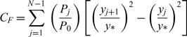 $$\begin{equation}
C_{F} =\sum _{j=1}^{N-1}\; \left(\frac{P_{j} }{P_{0} } \right) \left[\left(\frac{y_{j+1} }{y{*} } \right)^{2} -\left(\frac{y_{j} }{y{*} } \right)^{2} \right]
\end{equation}
$$
$$\begin{equation}
C_{F} =\sum _{j=1}^{N-1}\; \left(\frac{P_{j} }{P_{0} } \right) \left[\left(\frac{y_{j+1} }{y{*} } \right)^{2} -\left(\frac{y_{j} }{y{*} } \right)^{2} \right]
\end{equation}
$$
6.0 ERROR CAUSED BY THE NUMERICAL PROCESS
To have a convergence, the critical section ratios given by (13) and (34) are compared using the expression (35):
 $$\begin{equation}
\varepsilon _{(A_{E} /A{*} )} (\% ) = \left| 1 - \frac{(A_{E} /A{*} )_{Computed} }{(A_{E} /A{*} )_{Exact} } \right| \times 100
\end{equation}
$$
$$\begin{equation}
\varepsilon _{(A_{E} /A{*} )} (\% ) = \left| 1 - \frac{(A_{E} /A{*} )_{Computed} }{(A_{E} /A{*} )_{Exact} } \right| \times 100
\end{equation}
$$
If ε is less than the desired precision, we can consider that there is a convergence of the results
7.0 RESULTS AND COMMENTS
The presentation of the results is done for the two 2D and axisymmetric geometries according to the use of the nozzle. For aerospace construction, one is interested in the axisymmetric, and for wind tunnel construction, the 2D.
The presented design results are the nozzle shape and the numerical design parameters L/y∗, CMass, C F and y E/y∗. All five parameters depend essentially on M E, T 0, P 0 and the chosen gas (C P(T, ρ), a, b and α) as well as the type of 2D or axisymmetric geometry. Except the C F, which does not depend on the geometry. That is to say, it is the same between the 2D and axisymmetric geometries.
The comments concerning the variation of the five parameters with M E, T 0 and P 0 is the same between the 2D and axisymmetric cases. Except the numerical values, which change with the data.
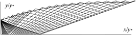
Figures 3 and 7 show a typical example of a characteristic mesh respectively in the axisymmetric and 2D nozzle generated by our developed program. The three regions of Figure 1 are well presented. It should be noted that the numerical results on the design parameters depend on the mesh used in the calculation. The latter depends on three parameters, which are the incrementation of the deflection angle of the flow between two successive Mach lines in the Kernel region. The incrementation of the characteristics in the transition zone for the axisymmetric case, as well as the number of additional characteristics after the sonic line OA. Our results are controlled by the convergence of the critical section ratios given by (34) concerning the chosen mesh, to the exact value given by relation (13). In the applications, we have chosen a precision better than ε = 10−4.

Figure 3. Mesh in axisymmetric MLN.
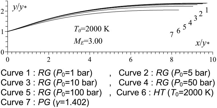
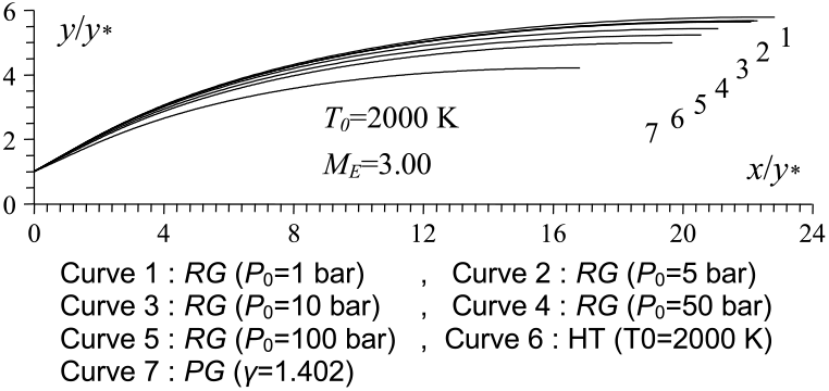
Figure 4. P0 effect on the RG axisymmetric MLN design.
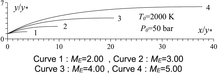
Figure 5. M E effect on the RG axisymmetric MLN design
Figure 6. T 0 effect on the RG axisymmetric MLN design.
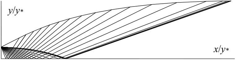
Figure 7. Mesh in 2D MLN.
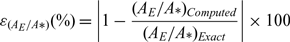
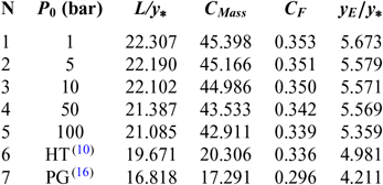
Figures 4 and 8 show the effect of P 0 on the contour of the axisymmetric and 2D MLN, giving M E = 3.00 at the exit when T 0 = 2, 000 Kelvin. Five values of P 0 were taken and are 1.0 bar, 5.00 bar, 10.0 bar, 50.0 bar and 100.0 bar. In these figures, the contour profiles for the same data for the PG(Reference Emanuel and Argrow3,Reference Anderson16) and HT(Reference Zebbiche9,Reference Zebbiche and Youbi10) models were added for comparison purposes. The corresponding numerical design results are presented in respectively in Tables 1 and 2. The influence of P 0 on the nozzle contour and on all the design parameters is clearly visible. In this case, the size of the nozzle given by our model RG is quite large compared to the size of the nozzles given by the PG and HT models, whatever the value of P 0. This result is very advantageous making it possible to say that in order to have a complete expansion inside the nozzle according to the real gas flow behaviour, a large space of the nozzle is required compared to that given by the PG and HT models. These two models reduce the shape of the nozzle relative to the actual need for the gas flow behaviour. The value of P 0 of the combustion chamber in reality must take a precise value. For this reason, its influence is remarkable in all the design parameters.

Figure 8. P 0 effect on the RG 2D MLN design.
Table 1 Design values for the nozzles of Figure 4

Table 2 Design values for the nozzles of Figure 8
It is estimated that the problem of the existence of side loads during the out-of-adaptation regime will be considerably reduced and will be justified by the wind tunnel tests.
If, for example, the MOC HT model is used to determine the flow parameters in the nozzle sized by the RG model, we will find an increase in M E compared to that desired in the design by the RG model, and in particular, a difference in all the parameters between those found in the calculation and the design results. In addition, the configuration shown in Figure 1 will not be respected; in other words, the absence of the uniform zone in particular. It is the same remark if we use the PG model instead of RG model. In this case, the difference between the parameters given by the PG and RG models is quite high, given the difference in the space of the flow found between the suitable nozzles given by the two models. Thus, more is bigger, plus the expansion will be great and an increase of M E is remarkable.
Now, if one uses the present MOC RG model to calculate the flow in the nozzle sized on the basis of the HT or PG model, the gas will find a reduced space, which will influence considerably the behaviour of gases, and an oblique shockwaves will be appear in the nozzle despite the fact that the nozzle is adapted in the direction of HT or PG. We will notice that the adaptation of the nozzle, actually of the nozzle, will be for an NPR large enough compared to that found by the HT and PG models, and it will give us an increase in the zone of the side loads paining with considerable amplitude. So, as a solution, it is necessary to respect properly the behaviour of gas during the flow by taking into account good hypotheses bringing the maximum possible towards the reality.
In the international community, the design results given by our RG model cannot currently be verified by existing CFD codes, as they are developed on the basis of the consideration of the state equation of perfect gas (P = ρRT) and not on the consideration of the hypotheses of a real gas. The only way to validate the design results of our RG models through the verification with wind tunnel experiment.
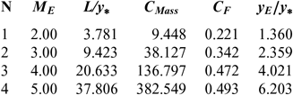
Figures 5 and 9 show the effect of M E respectively on the shape of the axisymmetric and 2D MLN, determined by our model RG when T 0 = 2, 000 K and P 0 = 50 bar. The example taken is for M E = 2.00, 3.00, 4.00 and 5.00. The design results in the RG framework are shown respectively in Tables 3 and 4. For comparison purposes, only the numerical design results of the same nozzles in the HT model(9,10), respectively present in Tables 5 and 6, and the design results for PG model(3,16), as shown in Tables 7 and 8, were presented. It should be noted that the shape of the nozzles given by the PG and HT models are different from those presented in Figures 7 and 8. It is clearly noticed again is the effect of M E on the MLN shape. What disrupts the M E is also an important parameter for our RG model.
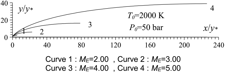
Figure 9. M E effect on the RG 2D MLN design.
Table 3 RG design values for the nozzles of Figure 5

Table 4 RG design values for the nozzles of Figure 9
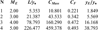
Table 5 HT design values(9) for the nozzles of Figure 5
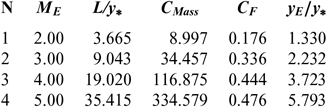
Table 6 HT design values(10) for the nozzles of Figure 9
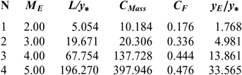
Table 7 PG design values(3) for the nozzles of Figure 5
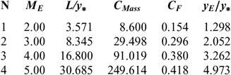
Table 8 PG design values(16) for the nozzles of Figure 9
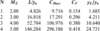
Note in Figures 5 and 9 and Tables 3-8, that according to the variation of M E, the design results given by the RG model are all superior to the design results given by the HT model, and both models are superior to the results of PG model. Then, the PG and HT models make a default design of the nozzle that will influence the flow quality and the physical interpretation of actual flow behaviour.
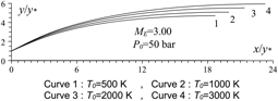
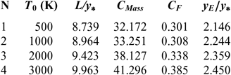
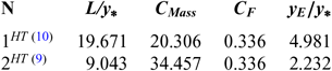
Figures 6 and 10 show the effect of T 0 respectively on the shape of the axisymmetric and 2D MLN, determined by our RG model when P 0 =50 bar and M E =3.00. The example taken is for T 0 =500K, 1,000K, 2,000K and 3,000K. The numerical design results in the context of real gas are presented respectively in Tables 9 and 10. For comparison purpose, we added only the numerical design results of the same nozzles in the framework of the HT model(Reference Zebbiche9,Reference Zebbiche and Youbi10) , as presented the Tables 11 and 12, and the design results in the framework of the PG model(Reference Emanuel and Argrow3,Reference Anderson16) , as presented the Tables 13 and 14. It should be noted that the nozzle shape given by the PG and HT models are different from those presented in Figures 6 and 10. It is clearly noticed again the effect of T 0 on theMLN shape. What disrupts that T 0 is also an important parameter in our RG model.
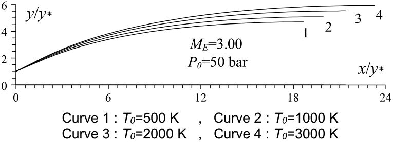
Figure 10. T 0 effect on the RG 2D MLN design.
Table 9 RG design values for the nozzles of Figure 6

Table 10 RG design values for the nozzles of Figure 10
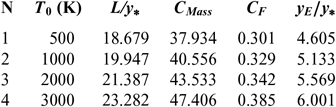
Table 11 HT design values(9) for the nozzles of Figure 6
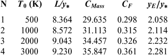
Table 12 HT design values(10) for the nozzles of Figure 10
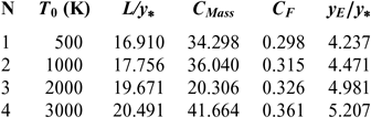
It is noted in Figures 6 and 10 and Tables 9-14, that according to the variation of T 0, the design results given by the RG model are all superior to the design results given by the HT model, and both models are superior to the results of PG model. Then, the PG and HT models make a default design of the nozzle that will influence the flow quality and the physical interpretation of actual flow behaviour.
Table 13 PG design values(3) for the nozzles of Figure 6
Table 14 PG design values(16) for the nozzles of Figure 10
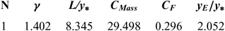
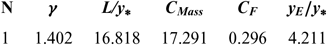
For the PG model, the design results do not depend on T 0 and P 0. For this reason, we find only a value of each parameter according to the value of γ, which is taken to γ = 1.402 as presented in Tables 13 and 14.
For each parameter of our five design parameters, the RG results are found to be different from the HT and PG results due to the fact that the P 0 is taken into account in our RG model.
Figure 11 shows the influence of 2D and axisymmetric geometries on the MLN shape in the context of our RG model when P 0 = 50 bar and M E = 3.00 and T 0 = 2000 K as well as a comparison between the HT and PG models, followed by the design parameters as shown in Table 15 for the RG model, Table 16 for the HT model and Table 17 for the PG model. It is clearly remarkable the influence of P 0 on the RG model and the difference between the five design parameters between the three models. It should be noted that the C F is the same for 2D and axisymmetric geometry and only varies with M E, T 0 and P 0. But the other parameters vary in addition to the 2D and axisymmetric geometry.
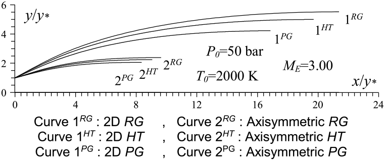
Figure 11. Axisymmetric and 2D MLN comparison.
Table 15 RG design values for the nozzles of Figure 11
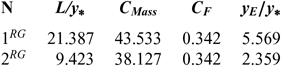
Table 16 HT design values for the nozzles of Figure 11

Table 17 PG design values for the nozzles of Figure 11
Considering Fig. 11 and the results presented in Tables 15-17, we can say that it is recommended to use axisymmetric geometry for aerospace construction and 2D geometry for wind tunnel construction. For aerospace construction, the criteria to be followed is to choose a nozzle of propulsion with the smallest C Mass and, in parallel, the greatest possible C F and M E. While for blowers, it is desired to have a ratio of critical sections (A E/A∗) as large as possible. In parallel, it is recommended to have the smallest temperature distribution (T E/T 0) at the exit of the nozzle to tune the prototype of the aerospace machine without detaching the measurement instruments, demonstrating the influence of the geometry of the nozzle for use in aerospace or wind tunnel construction. In some cases, it is quite advisable to calculate the fineness for the aerospace and wind tunnel construction, respectively, by the following two relations f = (C F × M E)/C Mass and f = (A E/A∗)/(T E/T 0). So, a good nozzle for both constructions is one that has the greatest fineness possible.
8.0 CONCLUSION
This work enabled us to develop a new model of MOC based on the stagnation pressure effect on the design of 2D and axisymmetric MLN. This study is presented for the use of the RG phenomenon. The Berthelot state equation is used for application. The following conclusions are obtained:
1 The stagnation pressure P 0 is an important parameter for our RG model. It increases the size of the nozzle compared to those given by the HT and PG models.
2 The numerical results are controlled by the convergence of A E/A∗ calculated numerically by (34) towards Equation (13).
3 The computer execution time for the RG model is quite large compared to that given by the PG and HT models.
4 For the given M E, T 0, y∗, an infinity of contours can be found by varying P 0.
5 For the PG and HT models, all the physical parameters can be obtained as a function of one state variable M or T, respectively. For our RG model, all the physical parameters depend on two state variables T and ρ.
6 The PG and HT models become a particular case of our RG model. They can be obtained by taking (a = b = α = 0) and (a = b = 0, α ≠ 0), respectively.
7 The Berthelot state equation is taken for our presented RG model of MOC.
As prospects, determine the stagnation pressure P 0 effect on the 2D and axisymmetric plug and expansion deflexion nozzles and the dual bell nozzle by using the presented MOC RG model to improve the design parameters compared to that given by the HT and PG models. Develop a CFD calculation code based on the consideration of our RG model in order to verify the design calculations given by MOC.