


1. Introduction
Different physical mechanisms have been proposed to explain so-called ‘rogue’ waves on the surface of the ocean (Dysthe, Krogstad & Müller Reference Dysthe, Krogstad and Müller2008; Kharif, Pelinovsky & Slunyaev Reference Kharif, Pelinovsky and Slunyaev2008; Onorato et al. Reference Onorato, Residori, Bortolozzo, Montina and Arecchi2013; Adcock & Taylor Reference Adcock and Taylor2014; Dudley et al. Reference Dudley, Genty, Mussot, Chabchoub and Dias2019). Rogue waves are typically defined as large waves whose height exceeds the significant wave height by a factor of 2–2.2 (Kharif et al. Reference Kharif, Pelinovsky and Slunyaev2008). Such waves are of increased interest if they occur more frequently than predicted by a Gaussian process. A useful proxy for rogue waves therefore is the excess kurtosis of the free surface relative to a Gaussian process (Mori & Janssen Reference Mori and Janssen2006). Physical mechanisms proposed include random linear dispersive focusing enhanced by weak bound-wave nonlinearity (Fedele et al. Reference Fedele, Brennan, De León, Dudley and Dias2016), modulational or Benjamin–Feir instability in deep water (Benjamin & Feir Reference Benjamin and Feir1967; Janssen Reference Janssen2003), and abrupt depth transitions (ADTs), among others.
Recently, several authors have shown that rogue waves can form at the top of ADTs for waves in shallow to intermediate depth, as reviewed in Trulsen et al. (Reference Trulsen, Raustøl, Jorde and Bæverfjord Rye2020). In the experiments of Trulsen, Zeng & Gramstad (Reference Trulsen, Zeng and Gramstad2012), local peaks of skewness and kurtosis occurred a short distance after a 1 : 20 underwater slope when waves travelled from a deeper to a shallower domain (see also Zhang et al. Reference Zhang, Benoit, Kimmoun, Chabchoub and Hsu2019). Similar peaks have been observed experimentally for shoals (Ma, Dong & Ma Reference Ma, Dong and Ma2014; Trulsen et al. Reference Trulsen, Raustøl, Jorde and Bæverfjord Rye2020) and steps (Bolles, Speer & Moore Reference Bolles, Speer and Moore2019). Local peaks in skewness and kurtosis have also been predicted using reduced-form nonlinear evolution equations, such as the Korteweg–de Vries equation for variable shallow depth (Sergeeva, Pelinovsky & Talipova Reference Sergeeva, Pelinovsky and Talipova2011; Majda, Moore & Qi Reference Majda, Moore and Qi2019) and the Boussinesq equations (Gramstad et al. Reference Gramstad, Zeng, Trulsen and Pedersen2013; Kashima, Hirayama & Mori Reference Kashima, Hirayama and Mori2014; Zhang et al. Reference Zhang, Benoit, Kimmoun, Chabchoub and Hsu2019), and by fully nonlinear numerical simulations of the water wave equations (Viotti & Dias Reference Viotti and Dias2014; Ducrozet & Gouin Reference Ducrozet and Gouin2017; Zheng et al. Reference Zheng, Lin, Li, Adcock, Li and van den Bremer2020; Zhang & Benoit Reference Zhang and Benoit2021). The magnitude of the peaks is greatest when the ADT is infinitely steep, i.e. a step (Zheng et al. Reference Zheng, Lin, Li, Adcock, Li and van den Bremer2020). Peaks in skewness and kurtosis only occur for sufficiently shallow depths (Trulsen et al. Reference Trulsen, Raustøl, Jorde and Bæverfjord Rye2020; Zheng et al. Reference Zheng, Lin, Li, Adcock, Li and van den Bremer2020), corresponding to a depth beyond the applicability of the nonlinear Schrödinger equation (Zeng & Trulsen Reference Zeng and Trulsen2012), which correctly predicts the absence of peaks in deeper water (Lawrence, Trulsen & Gramstad Reference Lawrence, Trulsen and Gramstad2021).
Two hypotheses have been proposed to explain these peaks. According to the first, ADTs place the system out of equilibrium; the peaks are the response of a system that rapidly adjusts to a new equilibrium driven by nonlinear processes (third- and higher-order in steepness) (Trulsen Reference Trulsen2018; Viotti & Dias Reference Viotti and Dias2014). According to the second hypothesis, the peaks are formed by second-order effects in steepness (Gramstad et al. Reference Gramstad, Zeng, Trulsen and Pedersen2013; Ducrozet & Gouin Reference Ducrozet and Gouin2017; Zhang et al. Reference Zhang, Benoit, Kimmoun, Chabchoub and Hsu2019; Zheng et al. Reference Zheng, Lin, Li, Adcock, Li and van den Bremer2020), but the mechanism by which this occurs is not clear.
We develop a statistical model, based on the second-order theory for wave propagation over a step that was developed in Li et al. (Reference Li, Zheng, Lin, Adcock and van den Bremer2021b) and validated experimentally in Li et al. (Reference Li, Draycott, Adcock and van den Bremer2021a), that can accurately predict the magnitude and location of the peaks in kurtosis atop ADTs. Our model confirms the validity of the second hypothesis and demonstrates that the underlying mechanism is one of the interplay between linear free and second-order bound waves, which are also present in the absence of the ADT, and the second-order free waves generated due to the ADT.
2. Theoretical model
2.1. Deterministic model (Li et al. Reference Li, Zheng, Lin, Adcock and van den Bremer2021b)
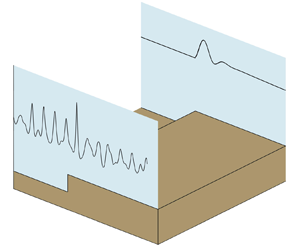
Our starting point is the deterministic model of Li et al. (Reference Li, Zheng, Lin, Adcock and van den Bremer2021b) for wave group propagation over a step. We consider weakly nonlinear unidirectional water waves on the surface of a constant-density fluid, ignoring surface tension and viscosity, so that the fluid satisfies potential flow. The ADT (cf. figure 1) takes the form of a discontinuity or ‘step’ in water depth  $h(x)$ at
  $x =0$, where
  $h$ changes from
  $h_d$ for
  $x<0$ to a shallower value
  $h_s$ for
  $x>0$, with
  $x$ denoting the horizontal axis. We consider intermediate water depths (
 ${O}(kh)=1$ with
  $k$ the wavenumber) and leading-order approximations to the water wave equations. Specifically, as in the classical statistical models of Tayfun (Reference Tayfun1980, Reference Tayfun1986), the solutions are valid up to second order in steepness
  $\epsilon = k_0A_0$, where
  $k_0$ and
  $A_0$ denote the characteristic wavenumber and amplitude, respectively, and narrow-banded or valid up to first order in the dimensionless bandwidth parameter, defined as
  $\delta = 1/(k_0\sigma _0)$ with
  $\sigma _0$ the characteristic group length.

Figure 1. Experimental set-up.
2.1.1. Incident wave field
The surface elevation of the incident wave field travelling towards the ADT can be obtained from a combined Stokes and multiple-scales expansion (e.g. Mei, Stiassnie & Yue Reference Mei, Stiassnie and Yue1989):
 $$\begin{gather} \zeta(x,t) = \zeta^{(1)}(x,t) + \zeta^{(2)}(x,t)\quad \text{for}\ x<0,\ \text{with} \end{gather}$$
 $$\begin{gather}\zeta^{(1)}(x,t) = A\cos \psi_0(x,t)\quad \text{and}\quad {\zeta}^{(2)}(x,t) = ~ k_0A^2[C_{20,b}+C_{22,b}\cos2\psi_0(x,t)], \end{gather}$$
where the superscripts denote the order in  $\epsilon$;
  $A(x,t)$ the envelope; and
  $\psi _0 = k_0x -\omega _0 t+\theta _0$ the phase, with
  $k_0$ the carrier wavenumber and
  $\omega _0 =\omega (k_0,h_d)$ the angular velocity obeying linear dispersion,
  $\omega (k,h)= \sqrt {gk\tanh kh}$ with
  $g$ gravitational acceleration, and
  $\theta _0$ the phase. The envelope
  $A(x,t)=A(x/c_{g0}-t)$ travels at the group velocity
  $c_{g0} =c_g(k_0,h_d)$, with
  $c_g(k,h)=(\omega /(2k))(1+2kh/\sinh 2kh)$. The coefficients of the bound second-order sub-harmonic and super-harmonic waves are (e.g. Mei et al. Reference Mei, Stiassnie and Yue1989)
 $$\begin{gather} C_{20,b}(kh) = [(2gh - c_g^2 )/(2\sinh 2kh) + 2g c_g/\omega]/[4 (c_g^2 - g h)], \end{gather}$$
 $$\begin{gather}C_{22,b}(kh) = {\cosh kh (2\cosh^2 kh+1)}/{(4 \sinh^3kh)}, \end{gather}$$
where  $C_{20,b}(k_0h_d)$ and
  $C_{22,b}(k_0h_d)$ are the coefficients in (2.1), and we have further assumed the envelope is long relative to the water depth (as in Mei et al. Reference Mei, Stiassnie and Yue1989).
2.1.2. Transmitted wave field
Upon reaching the ADT ( $x=0$), the incident wave field is reflected and transmitted. We focus on the latter here. At first order in
  $\epsilon$, the carrier wave on the shallower side travels at speed
  $c_{g0s}=c_g(k_{0s},h_s)$, where
  $k_{0s}$ denotes the wavenumber that can be found by solving
  $\omega _0=\omega (k_{0s},h_s)$ and corresponds to a shorter wavelength. In addition, evanescent waves are generated in the vicinity of the step that vanish exponentially with distance away from the step. At second order in
  $\epsilon$, the sub-harmonic and super-harmonic bound waves associated with the transmitted wave field must change magnitude at the step, and additional free sub-harmonic and super-harmonic waves are generated, which, respectively, travel at the shallow-water speed
  $\sqrt {g h_s}$ or satisfy the linear dispersion relation for
  $\omega (k_{20s},h_s) =2\omega _0$ with
  $k_{20s}$ the wavenumber of the super-harmonic waves.
Based on Massel (Reference Massel1983), who derived expressions for both linear and second-order super-harmonic components for a monochromatic wave, and Li et al. (Reference Li, Zheng, Lin, Adcock and van den Bremer2021b), who extended this work to narrow-banded wavepackets, the surface elevation on the shallower side (i.e. for  $x>0$) is given by (Li et al. Reference Li, Zheng, Lin, Adcock and van den Bremer2021b)
 \begin{equation} \zeta_{s}(x,t)= \zeta_s^{(1)}(x,t) + \zeta_s^{(2)}(x,t)\quad \text{for}\ x>0, \end{equation}
with
 $$\begin{gather} {\zeta}^{(1)}_{s}(x,t)= A_s(x,t)\cos \psi_{0s} + {\zeta}^{(1)}_{Es},\quad A_s(x,t) = |T_0| A\left(x/c_{g0s}-t\right) , \end{gather}$$
 $$\begin{gather}{\zeta}^{(2)}_{s}(x,t) = \zeta^{(20)}_{s}+{\zeta}^{(22)}_{s}, \end{gather}$$
 $$\begin{gather}{\zeta}^{(20)}_{s}(x,t) = C_{{20},b} k_{0s} A_s^2 +C_{{20},f} k_{0s}|T_0|^2 A^2(x/\sqrt{g h_s}-t)+{\zeta}^{(20)}_{Es}, \end{gather}$$
and
 \begin{align} {\zeta}^{(22)}_{s}(x,t) &= C_{{22},b} k_{0s}A_s^2 \cos (2\psi_{0s}) + C_{{22},f} k_{0s}|T_0|^2 A^2(x/c_{g22s}-t) \cos (2\psi_{0s} + \psi_{{22,f}})\nonumber\\ &\quad + {\zeta}^{(22)}_{Es}, \end{align}
in which  $T_0$ denotes the complex transmission coefficient, and the subscripts
  $E$,
$E$,  $b$ and
  $f$ denote the evanescent, bound and free waves, respectively. In the first-order term,
  $\psi _{0s}(x,t) = \psi _0(x,t) + (k_{0s}-k_0)x + \theta _{T_0}$ with
  $\theta _{T_0}$ denoting the phase shift due to the step (
 $\theta _{T_0}=\arg (T_0)$). The second-order bound wave coefficients can be evaluated from (2.2):
  $C_{20,b}(k_{0s}h_s)$,
  $C_{22,b}(k_{0s}h_s)$. The second-order free wave coefficients are given by
  $C_{20,f} = |T_{20,f}|/|T_0|^2$ and
  $C_{22,f} = 2\omega ^2_0 |T_{22,f}|/(g k_{0s} |T_0|^2)$ with
  $T_{20,f}$ and
  $T_{22,f}$ the (complex) coefficients for the sub- and super-harmonic free wave, respectively.
  $T_{0}$,
  $T_{20}$ and
  $T_{22,f}$ are obtained from the boundary conditions at the step (see Li et al. (Reference Li, Zheng, Lin, Adcock and van den Bremer2021b) for details). In the second-order terms,
  $c_{g22s}=c_g(k_{20s},h_s)$ is the group velocity of the free super-harmonic envelope, and
  $\psi _{22,f}(x) =k_{20s}x-2k_{0s}x+\theta _{{T_{22,f}}} - 2\theta _{T_0}$ denotes the phase of the free super-harmonic waves relative to the bound super-harmonic waves, with
  $\theta _{{T_{22,f}}}$ the phase shift of the free super-harmonic waves upon transmission (
 $\theta _{T_{22,f}}=\arg (T_{22,f})$). To obtain tractable solutions, Li et al. (Reference Li, Zheng, Lin, Adcock and van den Bremer2021b) ignore forcing by (small) products of linear evanescent waves.
2.2. A new statistical model
To develop a statistical model based on the deterministic model of Li et al. (Reference Li, Zheng, Lin, Adcock and van den Bremer2021b) outlined in § 2.1, we assume a normally distributed linear incident field  $\tilde {\zeta }^{(1)}$ with variance
  $\mu _0$, which is both stationary and homogeneous (for
  $x<0$). Specifically, we define a Rayleigh-distributed envelope
  $\tilde {A}$ and a uniformly distributed phase
  $\tilde {\psi }$, so that
  $\tilde {\zeta }^{(1)}=\tilde {A}\cos (\tilde {\psi })$. Tildes denote random variables. The incident wave field on the deeper side (
 $x<0$) becomes (cf. (2.1))
 \begin{align} \tilde{\zeta} = \tilde{\zeta}^{(1)} + \tilde{\zeta}^{(2)}\ \text{for}\ x<0,\quad \tilde{\zeta}^{(1)} =\tilde{A}\cos \tilde{\psi},\quad \text{and}\quad \tilde{\zeta}^{(2)} =k_0\tilde{A}^2[C_{20,b}+C_{22,b}\cos 2\tilde{\psi}]. \end{align}
Neglecting the effect of evanescent waves, we obtain on the shallower side (cf. (2.3))
 \begin{equation} \tilde{\zeta}_s = \tilde{\zeta}_s^{(1)} + \tilde{\zeta}_s^{(2)}\quad \text{for}\ x>0, \end{equation}
with
 $$\begin{gather} \tilde{\zeta}^{(1)}_{s}= |T_0| \tilde{A} \cos (\tilde{\psi}_{0s})\quad\text{and}\quad \tilde{\zeta}^{(2)}_{s}(x) = \tilde{\zeta}^{(20)}_{s}(x)+\tilde{\zeta}^{(22)}_{s}(x), \end{gather}$$
 $$\begin{gather}\tilde{\zeta}^{(20)}_{s}(x) = k_{0s} |T_0|^2 \tilde{A}^2 \left(C_{{20},b}+C_{{20},f}R_{{20}} (x)\right), \quad \tilde{\psi}_{0s} = \tilde{\psi}+(k_{0s}-k_0)x+\theta_{T_0}, \end{gather}$$
and
 \begin{equation} \tilde{\zeta}^{(22)}_{s}(x) = k_{0s}|T_0|^2 \tilde{A}^2 [C_{{22},b}\cos (2\tilde{\psi}_{0s}) + C_{{22},f}R_{{22}}(x) \cos (2\tilde{\psi}_{0s} +\psi_{{22,f}}(x))], \end{equation}
where  $R_{{20}}(x)$ and
  $R_{{22}}(x)$ are envelope functions, obtained by expanding the envelope of the sub- and super-harmonic waves, respectively, about the centre of the transmitted envelope. They can be expressed in terms of the focused deterministic envelope
  $A$ as
 \begin{align} R_{{20}}(x)=A^{2}(x/\sqrt{g h_s}-x/c_{g0s})/A^{2}(0),\quad R_{{22}}(x)=A^{2}(x/c_{g22s}-x/c_{g0s})/A^{2}(0), \end{align}
where  $A(0)$ is the central magnitude of the deterministic envelope. The focused deterministic envelope can be obtained from the energy spectrum
  $S(\omega )$ by
  $A(t)=\int \sqrt {2S(\omega )}\cos ((\omega -\omega _0)t)\,\textrm {d}\omega$. For a Gaussian deterministic envelope
  $A=a_0 \exp (-c_{g0}^2(x/c_{g0s}-t)^2/(2\sigma _0^2))$, we obtain
  $R_{{20}}(x)= \exp [-(c_{g0} x/\sqrt {gh_s}-c_{g0}x/c_{g0s})^2/\sigma _0^2]$ and
  $R_{{22}}(x)= \exp [-(c_{g0} x/c_{g22s}-c_{g0}x/c_{g0s})^2/\sigma _0^2]$. A long distance away from the step,
  $R_{{20}},R_{{22}}\to 0$, and we recover the standard homogeneous result for constant depth (e.g. Tayfun Reference Tayfun1986).
2.2.1. Statistical properties
The skewness  $s=\langle (\tilde {\zeta }_s - m)^3\rangle /v^{3/2}$ and kurtosis
  $\kappa =\langle (\tilde {\zeta }_s - m)^4\rangle /v^{2}$ of the random surface elevation can be directly obtained from (2.5) with
  $m=\langle \tilde {\zeta }_s\rangle$,
  $v = \langle (\tilde {\zeta }_s - m)^2\rangle$ and
  $\langle \cdots \rangle$ the combined expectation operator of the random variables
  $\tilde {A}$ and
  $\tilde {\psi }$:
 $$\begin{gather} s = 6k_{0s}\sqrt{\mu_{0s}}C_{2}(x)+{O}(\mu^{3/2}_{0s}), \end{gather}$$
 $$\begin{gather}\kappa = 3 +24 k_{0s}^2 \mu_{0s} \left(\kappa_{{2,b}}+\kappa_{{2,bf}}(x)+ \kappa_{{2,f}}(x) \right) +{O}(\mu^2_{0s}). \end{gather}$$
Here  $\mu _{0s} = |T_0|^2\mu _0$ denotes the variance of the surface elevation on the shallower side,
  $C_{{2}}(x)= C_{{20},b} +C_{{22},b} + C_{{20},f}R_{{20}}(x) + C_{{22},f}R_{{22}}(x)\cos \psi _{{22,f}}(x)$,
  $\kappa _{{2,b}}$ captures the contribution to kurtosis by bound waves,
  $\kappa _{{2,f}}$ by free waves and
  $\kappa _{{2,bf}}$ by their combination:
 $$\begin{gather} \kappa_{{2,b}}=3 C^2_{{20},b} +4 C_{{20},b}C_{{22},b} + 3C^2_{{22},b}, \end{gather}$$
 $$\begin{gather}\kappa_{{2,f}}(x)=3 C^2_{{20},f}R_{{20}}^2 +4 C_{{20},f}C_{{22},f}R_{{20}}R_{{22}}\cos \psi_{{22,f}} + 3C^2_{{22},f}R_{{22}}^2, \end{gather}$$
 $$\begin{gather}\kappa_{{2,bf}}(x)= (6 C_{{20},b}+ 4C_{{22},b}) (C_{{20},f}R_{{20}}+C_{{22},f}R_{{22}}\cos\psi_{{22,f}}). \end{gather}$$
 From (2.5), we can also obtain a second-order accurate expression for wave crests  $\tilde {\zeta }_{c}$:
 \begin{equation} \tilde{\zeta}_c(x) = |T_0| \tilde{A} + k_{0s}|T_0|^2 \tilde{A}^2C_{{2}}(x). \end{equation}
In non-dimensional form,  $\tilde {\xi }_c=\tilde {\zeta }_c/H_{ss}$ with
  $H_{ss}=4\sqrt {\mu _{0s}}$ the significant wave height on the shallower side, the crest elevation has the probability density function (cf. Tayfun Reference Tayfun1980)
 \begin{equation} f_{\tilde{\xi}_c}(\xi_c)= \frac{16u\exp{({-}8u^2)}}{1+4\epsilon_s C_{{2}}(x)u}\quad \textrm{with}\ u=\dfrac{\sqrt{1+8\epsilon_s C_{{2}}(x)\xi_c}-1 }{4\epsilon_s C_{{2}}(x)}, \end{equation}
and  $\epsilon _s=k_{0s}H_{ss}/2$ measures steepness in a random sea. Equation (2.11a,b) can be integrated to obtain the exceedance probability (cf. Forristall Reference Forristall2000),
 \begin{equation} P(\tilde{\xi}_c>\xi_c)=\exp({-}8u^2(\xi_c)). \end{equation}
 As  $\epsilon _s\to 0$, we recover from (2.11a,b) and (2.12) the Rayleigh distribution. If the contributions by the second-order free waves are neglected, which is valid in the absence of, or a long distance away from, a step, then
  $R_{{20}}\to 0$ and
  $R_{{22}}\to 0$, and (2.5), (2.7), (2.8) and (2.10) reduce to the second-order accurate result for constant depth (Tayfun Reference Tayfun1980, Reference Tayfun1986).
2.2.2. Rogue wave generating mechanism
As described in § 2.1.2, second-order sub- and super-harmonic free waves are released upon transmission over the ADT. On the shallower side, these free waves coexist with the transmitted linear free waves and their second-order bound waves, which would also be present for constant depth. Compared to the second-order statistical model for constant depth (Tayfun Reference Tayfun1980, Reference Tayfun1986), the additional second-order free waves lead to an increased likelihood of large waves atop the ADT. The likelihood of large waves is enhanced by the presence of sub-harmonic free waves ( $C_{{20,f}}>0$) and beating between the bound and free super-harmonics, which results in local maxima (Li et al. Reference Li, Zheng, Lin, Adcock and van den Bremer2021b). Both these effects only occur near the top of an ADT, where the second-order free waves are initially generated and where their envelopes still overlap with the linear envelope. Since both sub-harmonics and super-harmonics propagate at different group speed from the linear envelope, they separate over a sufficient distance away from the step. This mechanism locally amplifies skewness (2.7), kurtosis (2.8) and exceedance probability of crests (2.12).
3. Results
3.1. Experiments and numerical simulations
To validate our statistical model, we performed laboratory experiments and fully nonlinear numerical simulations. Experiments were carried out in the Coastal, Ocean and Sediment Transport (COAST) Laboratory at the University of Plymouth, UK. A schematic of the experimental set-up (and the numerical wave tank) is shown in figure 1. Two water depths on the deeper side were used:  $h_d=0.55$ m and
  $h_d=0.75$ m. Hence, the water depth on the shallower side is
  $h_s = h_d -0.35$ m. The numerical wave tank (Zheng et al. Reference Zheng, Lin, Li, Adcock, Li and van den Bremer2020) is equivalent to that of the laboratory except that the computational domain has a total length of
  $50 \lambda _0$, where
  $\lambda _0$ denotes the carrier wavelength on the deeper side, with a length of
  $20 \lambda _0$ on the deeper side (
 $x<0$) and
  $30\lambda _0$ on the shallower side (
 $x>0$).
In both the experiments and the numerics, the (linear) wavemaker was programmed to generate irregular waves based on JONSWAP spectra for different peak frequencies  $f_p$ and water depths (peak enhancement factor
  $\gamma =3.3$). Four cases are examined with parameters presented in table 1. Cases A and C start in deeper water (
 $k_0h_d=1.6$) compared to B and D (
 $k_0h_d=1.0$,
  $1.1$), and cases A and B (
 $k_0h_d/(k_{0s}h_s)=1.9$,
  $1.8$) experience a larger depth transition than C and D (
 $k_0h_d/(k_{0s}h_s)=1.6$,
  $1.5$). We examine skewness and kurtosis (§ 3.2), followed by wave crest distribution (§ 3.3).
Table 1. Parameters of the laboratory experiments and fully nonlinear numerical simulations. The shallower water depth is  $h_s = h_d - 0.35$ m; the bandwidth is
  $\delta =1/(k_{0}\sigma _0)$;
  $H_{m0}$ is the measured significant wave height of the entire signal (the table shows its value obtained at the first gauge on the deeper side);
  $H_s=4\sqrt {\mu _0}$ is the significant wave height of the linearized surface elevation on the deeper side; the steepness is
  $\epsilon =k_0 H_s/2$;
  $\varGamma (kh)=\epsilon C_{22b}(kh)/(kh)^3$ denotes a parameter that measures the degree of nonlinearity relative to depth (Toffoli et al. Reference Toffoli, Monbaliu, Onorato, Osborne, Babanin and Bitner-Gregersen2007), with
  $C_{22,b}$ defined by (2.2b); and
  $N_1$ and
  $N_2$ denote the total number of the random realizations per case in experiments and numerical simulations, respectively.

For each case in table 1, several realizations with different randomized amplitudes and phases were generated in both experiments and numerical simulations. Random amplitudes and phases are generated for each frequency component as described in § 2.2. Each of these realizations was  $\sim$20 min (1200 s), with frequency spacing
  $\Delta f = 1/1800\ \textrm {Hz}$. The parameters used as input to the statistical model are estimated from the experimental values measured at the first gauge, before the step. For our (narrow-banded) model predictions, we have used an estimated, equivalent Gaussian envelope
  $A$ to compute the envelope functions
  $R_{{20}}(x)$ and
  $R_{{22}}(x)$.
3.2. Skewness and kurtosis
Figure 2 shows the spatial variation of skewness either side of the ADT ( $x=0$) for the four cases in table 1, including the step and the 1 : 1 and 1 : 3 slopes (for cases A and B). In all cases, the transition to a higher equilibrium value of skewness associated with larger bound waves for shallower depth is associated with sharp peaks. These sharp peaks, observed in previous studies, occur within one wavelength of the step. Their magnitudes and locations in both experiments and numerics, which are in good agreement, are predicted well by our statistical model. The non-uniform spatial resolution of experimental values is due to the limited number of gauges. We do not observe a significant difference between the experiments for a step and the 1 : 1 and 1 : 3 slopes, implying that the physics of steep slopes is captured well by our model. The largest peak is observed when the depth before the step is shallowest and the depth transition is greatest (case B).

Figure 2. Spatial variation of skewness  $s$, comparing theoretical prediction by (2.7), experiments and numerical simulations (‘FNPFS’) with
  $\lambda _{0s}$ the peak wavelength (step at
  $x=0$). The (small) error bars for the experiments and the thickness of the blue line for the numerics denote
  $\pm$ one standard deviation either side of the mean. Panels (a–d) correspond to the cases in table 1.
The only significant difference between the numerical simulations and our model in figure 2 arises in the region after the first peak, where we have few experimental observations (cases B and D), which agree better with the numerical simulations. These differences are likely due to violation of the narrow bandwidth assumption in our model for the broad-banded JONSWAP spectra we have used in the interest of realism, which causes the smearing out of the super-harmonic beating pattern. Figure 3 shows the spatial variation of kurtosis either side of the ADT ( $x=0$) for cases A–D. In all cases, the transmission over the ADT is associated with sharp peaks in kurtosis. In principle, two processes can contribute to kurtosis: third-order processes associated with modulational (in)stability that drive build-up of phase correlation of the linear signal (Janssen Reference Janssen2003) on the one hand and second-order bound and free waves on the other hand; both are captured by the experiments and the numerical simulations but only the latter by our statistical model. In the cases that are modulationally unstable before the ADT (A and C with
  $k_0 h_d=1.6>1.36$), the kurtosis in experiments and numerics starts slightly above the linear Gaussian value of
  $3$ with a negligible contribution by second-order bound waves. In all cases, the kurtosis in experiments and numerics gradually decays to an equilibrium value slightly below
  $3$ to the right of the ADT, corresponding to the modulationally stable conditions on the shallower side (
 $k_{0s}h_s<1.36$), where our second-order accurate statistical model only predicts a small positive contribution to kurtosis by bound waves (
 $R_{{20}}=R_{{22}}=0$ for
  $x\gg \sigma _{0s}$ with
  $\sigma _{0s}=\sigma _0c_{g0s}/c_{g0}$).

Figure 3. Spatial variation of kurtosis  $\kappa$, comparing theoretical prediction by (2.8), experiments and numerical simulations (‘FNPFS’) with
  $\lambda _{0s}$ the peak wavelength (step at
  $x=0$). The (small) error bars for the experiments and the thickness of the blue line for the numerics denote
  $\pm$ one standard deviation either side of the mean. Panels (a–d) correspond to the cases in table 1.
Crucially, the locations of the peaks in kurtosis are predicted accurately by our (second-order accurate) model in all cases. So are their magnitudes, with the relatively small differences between numerics and our model potentially arising because of third-order effects not included in our model, except for the deepest of our cases (case C, with  $k_sh_d=1.6$,
  $k_{0s}h_s=1.0$), for which these third-order effects are of the same order of magnitude as the (small) second-order peaks predicted by our model. Peaks are more significant when the water depth is shallower and the depth transition is greater. The kurtosis for the step and the 1 : 1 and 1 : 3 slopes is not significantly different.
3.3. Wave crest distribution
Figure 4 shows the exceedance probability distribution and the spatial variation of the probability of rogue waves, defined here as  $P(\tilde {\zeta }_c>1.25H_{m0})$ with
  $H_{m0}$ the measured significant wave height (of the entire signal), for case A (similar results are obtained for cases B–D). Very good agreement between the experiments, numerical simulations and theory is evident. In particular, the agreement is clear at the location of maximum rogue wave probability (gauge 5b). Minor differences in the rogue wave probability between, on the one hand, the theoretical predictions and, on the other hand, the experiments and numerics, which are in better agreement, can be observed close to the ADT (
 $0< x/\lambda _{0s}\lesssim 0.2$) and after the peak (
 $1 \lesssim x/\lambda _{0s}\lesssim 3$). The former is likely due to evanescent waves being neglected in our model, whereas the latter is primarily a result of the narrow-bandwidth assumption we have made (see Li et al. Reference Li, Zheng, Lin, Adcock and van den Bremer2021b).

Figure 4. Crest exceedance probability distribution at four locations (a) and the probability of rogue waves as a function of space (b) for case A, comparing the theoretical prediction by (2.12), experiments and numerical simulations (‘FNPFS’) (step at  $x=0$).
4. Conclusions
We have presented a statistical model to explain why rogue waves occur atop abrupt depth transitions (ADTs) in intermediate water depth. The model, based on Massel (Reference Massel1983) and Li et al. (Reference Li, Zheng, Lin, Adcock and van den Bremer2021b), includes nonlinearity up to second order in steepness, assumes narrow-banded irregular waves, represents the ADT as an infinitely steep step, and ignores the role of evanescent waves. We have validated our model through comparison to laboratory experiments and fully nonlinear numerical simulations of the water wave equations. In doing so, we have explained the mechanism behind the sharp peaks in kurtosis, indicative of rogue waves, atop ADTs recently observed by a large number of authors in experiments and numerical simulations (see e.g. Trulsen et al. (Reference Trulsen, Raustøl, Jorde and Bæverfjord Rye2020) and references therein). We show that peaks in kurtosis arise from the coexistence of linear free and second-order bound waves, which are also present in the absence of the ADT, and the second-order free waves additionally generated due to the ADT. As the second-order free waves always overlap with the linear waves near the top of the ADT but travel at different phase and group speeds (from the linear waves), the peaks are localized and the total wave field becomes inhomogeneous. Compared to (realistically broad-banded) numerical simulations and experiments, our (narrow-banded) model provides an accurate prediction of the spatially varying probability distribution of rogue waves and the associated peaks in skewness and kurtosis atop ADTs and identifies and explains a new physical mechanism by which rogue waves can arise in the ocean.
Funding
We acknowledge support from NSFC-EPSRC/NERC grants 51479114, EP/R007632/1, EP/R007519/1 and a Flexible Fund grant from the UK & China CORE. Y.L. acknowledges the support from the Research Council of Norway through the FRIPRO mobility project 287389. S.D. acknowledges a Dame Kathleen Ollerenshaw Fellowship. T.S.v.d.B. acknowledges a RAEng Research Fellowship. The authors would like to thank staff at the COAST laboratory.
Declaration of interests
The authors report no conflicts of interest.


