2. The model

Consider an OLG general equilibrium (macro)economy closed to international trade and inhabited by identical competitive firms and finite-lived rational and identical individuals (consumers/workers) of size 1 per generation. The assumption of identical agents allows us to refer to the choices of the representative individual and the representative firm throughout the article. The life of the representative individual is divided into youth (working period) and old age (retirement period). The members of generation t (t = 1, 2, … + ∞ is the time index) overlap for one period (youth) with the old members of generation t−1 and for one period (old age) with the young members of generation t + 1. When young, the individual is endowed with 1 unit of time and chooses how to allocate time endowment between labor (ℓ_t ∈ (0, 1)) and leisure (1 − ℓ_t) activities. The labor supply is offered to the competitive representative firm in exchange for wage w _t per unit of labor. The (total) labor income w _tℓ_t received during the working period is entirely saved (s _t) for old-aged consumption purposes (C _t+1). This assumption is usual in the related literature since the work of Reichlin (Reference Reichlin1986) and Galor and Weil (Reference Galor and Weil1996). Therefore, the budget constraint when young is:

(1)\begin{equation} s_{t} = w_{t}\ell _{t}. \end{equation}

When old, the individual retires and his accumulated wealth W _t+1 is:

(2)\begin{equation} W_{t + 1} = R_{t + 1}^{e}s_{t}, \end{equation}

where $R_{t + 1}^{e}$ is the interest factor that an individual of generation t expects will prevail from time t to time t + 1 (it will become the realised interest factor at the beginning of period t + 1). In this model, W _t+1 represents the potential consumption that could be achieved in the absence of any environmental damages (Weitzman, Reference Weitzman2010) and it is given by the overall amount of resources available to an individual during his retirement period. We assume that W _t+1 is reduced by environmental degradation D _t+1, and consumption C _t+1 is determined by the constraint:

(3)\begin{equation} C_{t + 1} = W_{t + 1}-\beta D_{t + 1} = R_{t + 1}^{e}w_{t}\ell _{t}-\beta D_{t + 1}, \end{equation}

where the parameter β ≥ 0 weights the importance of environmental degradation in the utility function. The term βD _t+1 can be interpreted as a damage function measuring the amount of wealth W _t+1 that must be used to repair the damages caused by environmental degradation D _t+1. So, the (net) wealth available for consumption purposes is given by W _t+1 − βD _t+1.Footnote ³

The individual representative of generation t has preferences towards leisure when young and material consumption when old, and his lifetime utility function takes the following form:

(4)\begin{equation} U_{t}=\ln (1-\ell _{t})+\theta \ln (C_{t+1}), \end{equation}

where 0 < θ < 1 is the subjective discount factor. The value of D _t+1 does not enter the utility function directly, but rather affects the need for the individual to increase his labor effort (and, consequently, the accumulation of wealth W _t+1) to keep the net wealth (i.e., consumption) W _t+1 − βD _t+1 unaltered.

Substituting out the expression of the lifetime budget constraint in (3) into the lifetime utility function (4) gives $U_{t}=\ln (1-\ell _{t})+\theta \ln (R_{t+1}^{e}w_{t}\ell _{t}-\beta D_{t+1})$ so that the individual optimization problem can be reduced to:

(5)\begin{equation} \max_{\ell _{t}}\ln (1-\ell _{t})+\theta \ln (R_{t+1}^{e}w_{t}\ell _{t}-\beta D_{t+1}). \end{equation}

We assume that the representative individual has perfect foresight about the value of D _t+1 but takes it as exogenously given. The first order condition for an interior solution reads as follows:

(6)\begin{equation} \frac{1}{1-\ell _{t}}=\frac{\theta R_{t+1}^{e}w_{t}}{R_{t+1}^{e}w_{t}\ell _{t}-\beta D_{t+1}}. \end{equation}

Equation (6) implies that an additional increase in the time spent working increases the marginal disutility of labor that should equate the (indirect) marginal utility of consumption coming from the resulting additional increase in net wealth to keep utility unchanged.

The representative firm produces a homogeneous good by means of the amount of labor available at time t (L _t) and the amount of saving rent by the representative individual to the firm at time t, which is invested in productive capital that will be installed one period later (K _t+1). Production takes place with a standard Cobb-Douglas technology mixing capital and labor inputs in the following way:

(7)\begin{equation} Y_{t}=AK_{t}^{\alpha }L_{t}^{1-\alpha }, \end{equation}

where Y _t is the output produced, A>0 is a production scaling parameter and 0 < α < 1 represents the elasticity of the production function with respect to the capital input. By assuming that the capital stock fully depreciates at the end of every period and output is sold at unit price, the maximization of profits $\Pi _{t}=AK_{t}^{\alpha }L_{t}^{1-\alpha }-R_{t}K_{t}-w_{t}L_{t}$ with respect to K _t and L _t implies that capital and labor are remunerated at their marginal products, respectively. Knowing that the temporary equilibrium condition in the labor market implies that labor demand equals labor supply, that is L _t = ℓ_t, marginal products of capital and labor can respectively be written in the following way:

(8)\begin{equation} R_{t}=\alpha A\left( \frac{K_{t}}{\ell _{t}}\right) ^{\alpha -1}, \end{equation}

and

(9)\begin{equation} w_{t}=(1-\alpha )A\left( \frac{K_{t}}{\ell _{t}}\right) ^{\alpha }. \end{equation}

The environmental damage at time t + 1 is determined by the following linear rule:

(10)\begin{equation} D_{t+1}=(1-\gamma )D_{t}+\delta \overline{Y}_{t}, \end{equation}

where 0 < γ ≤ 1 is the rate at which the damage decays over time, 1 − γ represents the degree of persistence of the damage in the environment and δ ≥ 0 weights the damage due to the economy-wide average production at time t ($\overline {Y}_{t}$). The lower (resp. higher) δ is, the more the technology is clean (resp. dirty).

The capital stock installed at time t + 1 equals aggregate investments by the representative firm, I _t, at time t, K _t+1 = I _t, which in turn are equal to aggregate savings by the representative individual s _t. By recalling that the capital stock fully depreciates at the end of each period, the market-clearing condition in the capital market is given by K _t+1 = s _t = w _tℓ_t. Knowing that individuals have perfect foresight, so that $R_{t+1}^{e}=R_{t+1}=\alpha AK_{t+1}^{\alpha -1}\ell _{t+1}^{1-\alpha }$, $\overline {Y}_{t}=Y_{t}$ (i.e., the economy-wide average output coincides, ex post, with the output of the representative firm) and using (6)–(10) one gets the following equations characterizing equilibrium dynamics of the economy:

(11)\begin{equation} K_{t+1}=(1-\alpha )AK_{t}^{\alpha }\ell _{t}^{1-\alpha }, \end{equation}

(12)\begin{equation} \frac{1}{1-\ell _{t}}=\frac{\theta \alpha (1-\alpha )A^{2}K_{t+1}^{\alpha -1}\ell _{t+1}^{1-\alpha }K_{t}^{\alpha }\ell _{t}^{-\alpha }}{\alpha (1-\alpha )A^{2}K_{t+1}^{\alpha -1}\ell _{t+1}^{1-\alpha }K_{t}^{\alpha }\ell _{t}^{1-\alpha }-\beta \lbrack (1-\gamma )D_{t}+\delta AK_{t}^{\alpha }\ell _{t}^{1-\alpha }]}, \end{equation}

and

(13)\begin{equation} D_{t+1}=(1-\gamma )D_{t}+\delta AK_{t}^{\alpha }\ell _{t}^{1-\alpha }. \end{equation}

The system formed by (11), (12) and (13) defines a three-dimensional map (M) characterising K _t+1 as a function of K _t and ℓ_t, and ℓ_t+1 and D _t+1 as functions of K _t, ℓ_t and D _t. Therefore,

(14)\begin{equation} M: \begin{cases} K_{t+1}=(1-\alpha )AK_{t}^{\alpha }\ell _{t}^{1-\alpha } \\ \ell _{t+1}=BK_{t}^{\frac{\alpha ^{2}}{\alpha -1}}\ell _{t}^{\frac{\alpha (1-\alpha )-1}{\alpha -1}}[\ell _{t}-\theta (1-\ell _{t})]^{\frac{1}{\alpha -1}}[(1-\gamma )D_{t}+\delta AK_{t}^{\alpha }\ell _{t}^{1-\alpha }]^{\frac{1 }{1-\alpha }},\\ D_{t+1}=(1-\gamma )D_{t}+\delta AK_{t}^{\alpha }\ell _{t}^{1-\alpha }, \end{cases} \end{equation}

where

(15)\begin{equation} B:=A^{({\alpha +1})/({\alpha -1})}\alpha ^{{\alpha }/({\alpha -1}) }(1-\alpha )^{{1}/({\alpha -1})}\beta ^{{1}/({1-\alpha})}. \end{equation}

3. The stationary state

The three equations in M allow us to compute the unique stationary-state solution of the system (K*, ℓ*, D*):

(16)\begin{equation} \ell ^{\ast }=\frac{\alpha \gamma \theta }{\alpha \gamma (1+\theta )-\beta \delta }, \end{equation}

(17)\begin{equation} K^{\ast }=[A(1-\alpha )]^{{1}/({1-\alpha })}\ell ^{\ast }, \end{equation}

(18)\begin{equation} D^{\ast }=\frac{\delta }{\gamma }A^{{1}/({1-\alpha })}(1-\alpha )^{{ \alpha}/({1-\alpha })}\ell ^{\ast }, \end{equation}

where the inequality αγ − βδ > 0 must hold to guarantee the positivity of all the variables of the model evaluated at the stationary state. In addition, the stationary-state solution of material consumption is the following:

(19)\begin{equation} C^{\ast }=\alpha \theta A^{{1}/({1-\alpha })}(1-\alpha )^{{\alpha }/({ 1-\alpha })}(1-\ell ^{\ast }). \end{equation}

Notice that if either β (the impact of environmental degradation on wealth) or δ (the impact of the economy-wide average production on environmental degradation) increases, then (ceteris paribus) labor input ℓ*, capital accumulation K* and environmental degradation D* increase. The opposite holds if the rate at which the damage decays over time, γ, increases. According to these results, we have that an increase in either β or δ, or a reduction in γ, induces individuals to work harder to counterbalance the increase in the damages caused by environmental degradation. This also explains, as we will show in the following sections, how the economy can follow an endogenous and self-fueling path characterized by growing defensive expenditures, environmental degradation, production growth, and wellbeing reduction.

Now, substituting out the stationary-state values (K*, ℓ*, D*) in (4), we get the stationary-state value of the lifetime utility function:

(20)\begin{equation} U_{ss}:=\ln (1-\ell ^{\ast })+\theta \ln (C^{\ast })=\ln \left\{ J^{1+\theta }\left[ \alpha \theta A^{{1}/({1-\alpha })}(1-\alpha )^{{\alpha }/({ 1-\alpha})}\right] ^{\theta }\right\}, \end{equation}

where J: = (αγ − βδ)/(αγ(1 + θ) − βδ) > 0 and, computing the partial derivatives of U _ss with respect to β, δ, and γ, we get:

\begin{equation*} \frac{\partial U_{ss}}{\partial \beta }=-\frac{\alpha \gamma \delta \theta (1+\theta )}{(\alpha \gamma -\beta \delta )[\alpha \gamma (1+\theta )-\beta \delta ]}<0, \end{equation*}

\begin{equation*} \frac{\partial U_{ss}}{\partial \delta }=-\frac{\alpha \beta \gamma \theta (1+\theta )}{(\alpha \gamma -\beta \delta )[\alpha \gamma (1+\theta )-\beta \delta ]}<0, \end{equation*}

\begin{equation*} \frac{\partial U_{ss}}{\partial \gamma }=\frac{\alpha \beta \delta \theta (1+\theta )}{(\alpha \gamma -\beta \delta )[\alpha \gamma (1+\theta )-\beta \delta ]}>0. \end{equation*}

This implies that an increase in the stationary-state values of labor supply ℓ*, capital accumulation K*, and environmental degradation D* due to an increase in either β or δ, or a reduction in γ, generates a reduction in the utility index evaluated at the stationary state.

Regarding the stability properties of the stationary state, (K*, ℓ*, D*) may be saddle-point stable, locally asymptotically stable or unstable. These cases occur when the Jacobian matrix evaluated at (K*, ℓ*, D*) has, respectively, two stable eigenvalues (i.e., inside the unit circle), three stable eigenvalues or less than one stable eigenvalue.

3.2. Locally asymptotically stable stationary state (local indeterminacy)

When the stationary state is locally asymptotically stable, there exists a multiplicity of trajectories converging towards (K*, ℓ*, D*), given an initial condition of the state variables (K, D) possibly close enough to (K*, D*). An interesting consequence of this outcome is that – once one has chosen the initial value of the control variable ℓ – the stationary state can be achieved through trajectories showing different economic performances and degrees of environmental degradation. An important role in the choice of the initial value of control variable is played by the expectations that agents have regarding the evolution of K and D (different expectations define different trajectories). This scenario is defined by the term local indeterminacy (Grandmont et al., Reference Grandmont, Pintus and de Vilder1998).

The stationary-state (K*, ℓ*, D*) may also not be attainable because all or ‘almost all’ trajectories diverge from it, and then converge towards other long-term scenarios. From a mathematical point of view, this case is observed when two or three eigenvalues are outside the unit circle.

It is easy to check that if either β = 0 or δ = 0, then the stationary state (K*, ℓ*, D*) is always saddle-point stable, and therefore it is locally determinate.Footnote ⁴ For β > 0 and δ > 0, the local stability properties of the stationary state (K*, ℓ*, D*) can be studied by accounting for the following local stability conditions (local indeterminacy):

(21)\begin{equation} \begin{cases} 1+a_{1}+a_{2}+a_{3}>0 \\ 1-a_{1}+a_{2}-a_{3}>0 \\ 1-a_{2}+a_{1}a_{3}-a_{3}^{2}>0 \\ 3+a_{1}-a_{2}-3a_{3}>0 \end{cases}, \end{equation}

where a ₁, a ₂ and a ₃ are, respectively, the coefficients related to the first-, second- and third-degree terms of the characteristic polynomial of the Jacobian matrix evaluated at the stationary-state. As the conditions in (21) cannot be dealt with in a neat analytical form, we will use numerical simulations in order to highlight some of the scenarios discussed above. Figure 1 shows, in the (β, δ)-plane, the determinacy/indeterminacy regions. The light-grey area identifies the parametric region where the stationary-state equilibrium is determinate, whereas the dark-grey area represents the region where local indeterminacy arises. The red line at the top of the dark-grey area identifies the boundary under which the stationary state exists (that is, αγ − βδ = 0). According to figure 1, an increase either in β or in δ may give rise to a local indeterminacy scenario, under which the transition dynamics towards (K*, ℓ*, D*) depends on the initial choice of the control variable.

Figure 1. Determinacy/indeterminacy in the (β, δ)-plane. Parameter set: A = 10.6, α = 0.3, γ = 0.64 and θ = 0.2.

Figure 2 illustrates two trajectories (dashed line and solid line) that start from the same values of the state variables K and D and converge towards the unique stationary state through different paths. The lifetime utility U _t of generation t behaves differently along the two trajectories, with some values of t in which U _t is higher along one trajectory, and others in which U _t is higher along the other trajectory. It may be interesting to observe that the discounted sum of utilities $Z:=\sum_{n=0}^{+\infty }\theta ^{n}U_{n}$ is lower along the dashed trajectory, which starts from a higher initial value of ℓ (Z _solid = −0.8282986747 > Z _dash = − 1.092149136). The same holds for the non-discounted sum $Q_{t}:=\sum_{n=0}^{t}U_{n}$ for every value of t (see figure 3). Therefore, if individuals can coordinate themselves by choosing a lower initial value of ℓ, which also implies a lower adaptation effort in the second period of life, then their choices allow the economy to follow a trajectory characterized by a higher wellbeing. Interestingly, the trajectory associated with the highest wellbeing (solid) corresponds to the lowest average value of the labor supply and lowest average value of defensive expenditures.

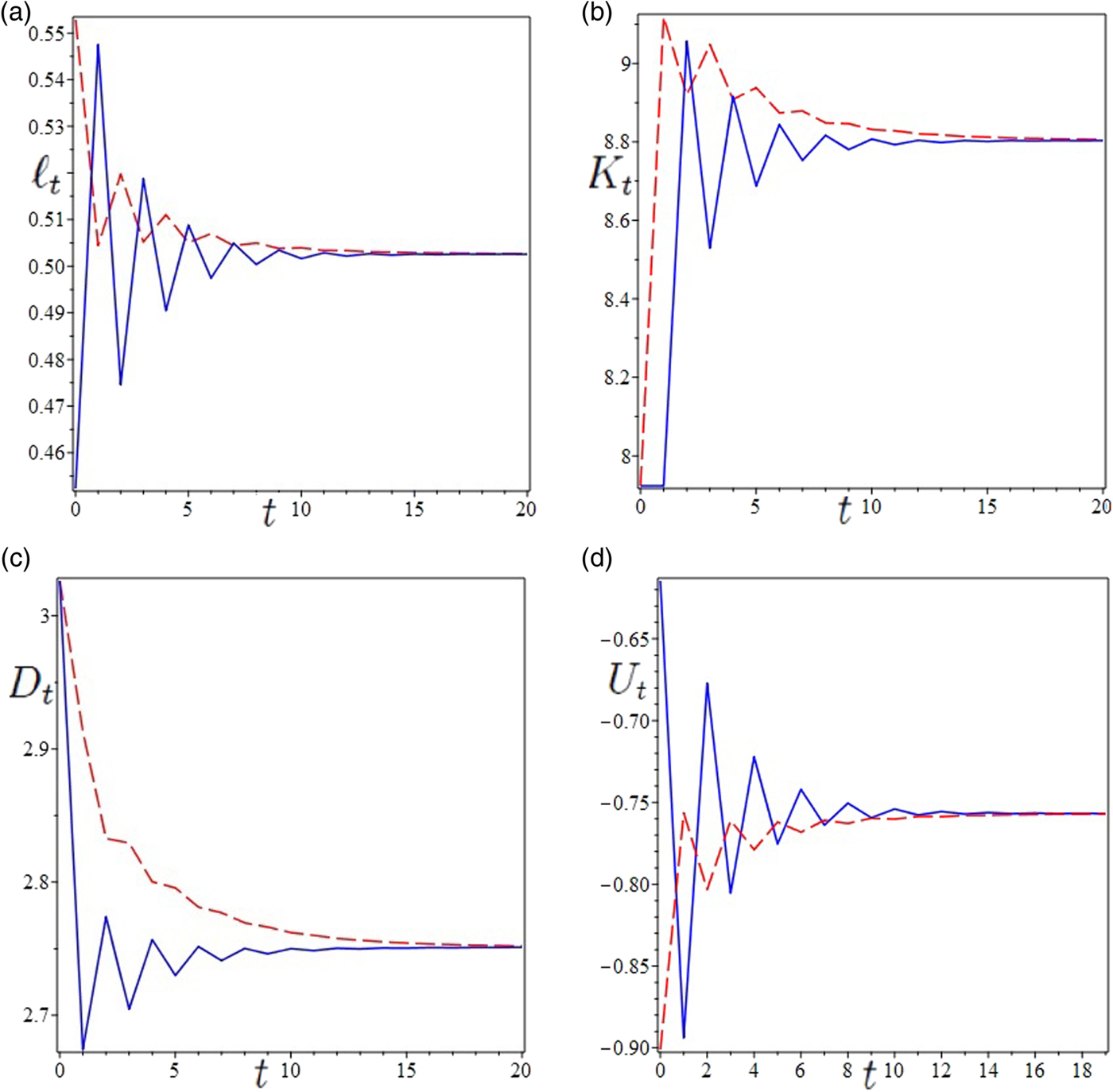
Figure 2. Local indeterminacy. Parameter set: A = 10.6, α = 0.3, γ = 0.64, θ = 0.2, δ = 0.14 and β = 1.1.

Figure 3. Values of $Q_{t}:=\sum_{n=0}^{t}U_{n}$ along the dashed and solid trajectories of figure 2. Parameter set: A = 10.6, α = 0.3, γ = 0.64, θ = 0.2, δ = 0.14 and β = 1.1.

In concrete terms, this result suggests that an increase in the degree of vulnerability to environmental degradation (β, i.e., the impact of environmental degradation on wealth) or an increase in the rate of output pollution intensity (δ, i.e., the impact of production on the environment) increases the likelihood of coordination failure. Individuals choose their initial labor supply based on their expectations on K and D but convergence towards the stationary state of the economy may occur through multiple paths. Therefore, the assumption of perfect foresight does not ensure agents' coordination as instead would be under saddle-point stability.

Given the initial conditions (history) and regardless of the initial value of the control variable (expectations), local asymptotic stability implies that the economy will eventually converge to the same long-term values of production, environmental quality, utility and wealth allocation between material consumption and defensive expenditures. However, this does not mean that the initial value of the control variable, the labor supply, is not relevant. As was pinpointed in the wellbeing analysis reported in this section, it may indeed have relevant consequences from a policy perspective.

4. Global indeterminacy

Despite the simplicity of the model, and the existence of only one stationary state, the interplay between production and consumption choices on the one hand and environmental degradation on the other may give rise to scenarios characterized by a high degree of complexity. If we do not concentrate only on the local properties of the dynamics around the stationary state but consider also the global properties of the system, it is possible to observe global indeterminacy. Global indeterminacy implies that two economies starting from the same initial conditions on the state variables K and D (history) can experience completely different development trajectories and long-term outcomes if they start from different initial values of the control variable ℓ. As was mentioned above, the initial choice of ℓ is determined by individual expectations about the future evolution of K and D (expectations matter). From a mathematical point of view, global indeterminacy implies a peculiar form of multistability for which there exists at least a pair $(\bar {K},\bar {D})$ such that two or more basins of attraction of the different attractors of the model are simultaneously cut by a plane defined by the conditions $K= \bar {K}$ and $D=\bar {D}$ at the same time.

An interesting scenario is the one in which global indeterminacy coexists with local determinacy. In this regard, an example is illustrated in figure 4, which depicts the time evolution of ℓ along two different trajectories. One of them approaches the stationary state (the dashed trajectory), which is saddle-point stable, and the other one approaches an attractive two-period cycle (the solid trajectory). These limit sets are achieved starting from the same value of the state variables (K ₀ = 1.67233424156157, D ₀ = 3.47754228557942) and fixing the initial conditions of the control variable at the values $\ell _{0}=\ell _{0}^{s}:=0.465776499615603$ and $\ell _{0}=\ell _{0}^{s}+0.1$, respectively. Though the stationary state is saddle-point stable, in this case the local analysis can be misleading as the economy may converge towards an attractor around the stationary state for infinite initial values ℓ₀ different from $\ell _{0}^{s}$.

Figure 4. Parameter set: A = 10.6, α = 0.3, $\beta = 0.89$, γ = 0.64, δ = 0.14 and θ = 0.2. Time series of two distinct trajectories of ℓ_t: one approaches the stationary state (dashed), which is saddle-point stable; the other approaches an attractive two-period cycle (solid).

Another scenario of global indeterminacy is illustrated in the bifurcation diagram depicted in figure 5 (panel a), showing the possible ω-limit sets for β ∈ (0.25, 0.45). The dashed line represents the stationary state, when it is saddle-point stable (local determinacy). The stationary state becomes attractive (local indeterminacy) for values of β approximately higher than 0.40 (the curve drawn in black). Starting from β = 0.25, the (locally determinate) stationary state is the unique existing ω-limit set. In this context, there is no global indeterminacy. For higher values of β (approximately β > 0.28) we can observe the rise of a chaotic attractor (the points in black), which coexists with the locally determinate stationary state. When β further increases, the chaotic attractor exhibits a sequence of reversed flip-bifurcations (period halving) leading to the scenario in which the (locally determinate) stationary state coexists with an attractive two-period cycle and eventually to the existence of a unique attractive stationary state (local indeterminacy). In addition, for β ranging approximately in the interval (0.302, 0.306) there exists another chaotic attractor (depicted in red). Therefore, for β ∈ (0.302, 0.306) we observe the coexistence amongst the locally determinate stationary state (dashed), an attractive two-period cycle (black) and the chaotic attractor (red). In this context of global indeterminacy, we have that starting from the same initial conditions of the state variables, three different long-term outcomes can be achieved depending on the initial choice of the control variable (ℓ).

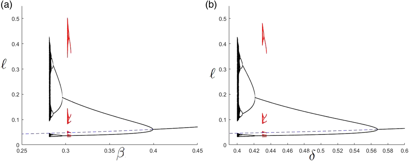
Figure 5. (a) Bifurcation diagram for β. Parameter set: A = 0.3, α = 0.33, γ = 0.9, θ = 0.03 and δ = 0.4. (b) Bifurcation diagram for δ. Parameter set: A = 0.3, α = 0.33, γ = 0.9, θ = 0.03 and β = 0.28131. Multiple coexisting ω-limit sets.

Figure 6 shows the time series of K, ℓ and D exhibiting the erratic behavior of a trajectory approaching the chaotic attractor illustrated in the bifurcation diagram of figure 5 (panel a) for β = 0.281310. Interestingly, the erratic trajectories in figure 6 are related to a lower average utility and a higher average labor supply than the corresponding stationary-state values. In other words, a strong effort for adaptation strategies can be detrimental for the environment, thereby inducing further adaptation and environmental degradation and then utility losses. The same results can be obtained if, ceteris paribus, the parameter δ changes (figure 5, panel b). For values of δ smaller than (around) 0.4, the long-term equilibrium is unique and determinate. This suggests that high values of δ not only produce a direct environmental damage but can also jeopardize agents' coordination leading to global indeterminacy. Therefore, policy makers should encourage the use of clean technologies.

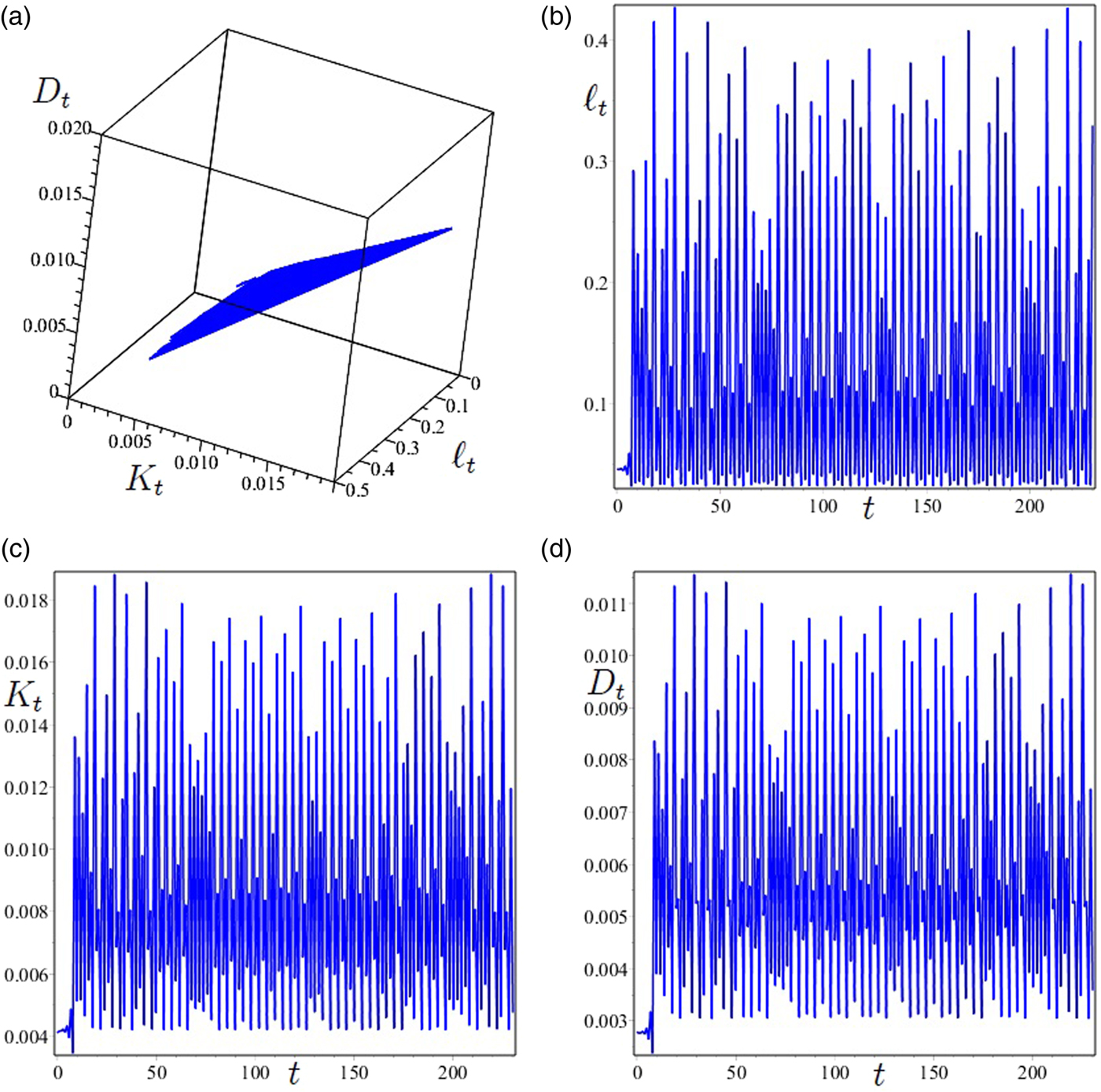
Figure 6. Parameter set: A = 0.3, α = 0.33, γ = 0.9, θ = 0.03 and δ = 0.4. Time series of the variables K, ℓ and D showing the erratic behavior of a trajectory approaching the chaotic attractor, illustrated in the bifurcation diagram of figure 5, for β = 0.281310.